Introduction
Detection of faults in rotating machinery is an important engineering task (Randall, 2011). Automatic fault diagnosis of complex machin-ery has economical and security related ad-vantages. Identifying a fault in its initial stage allows the early replacement of damaged parts (Wandekokem et al., 2011). This type of predic-tive maintenance is better than the prevenpredic-tive counterpart, which replaces parts that are not necessarily defective. Supervised learning is a machine learning approach widely used in automatic fault diagnosis (Xia et al., 2012; Liu, 2012; Wu et al., 2012).
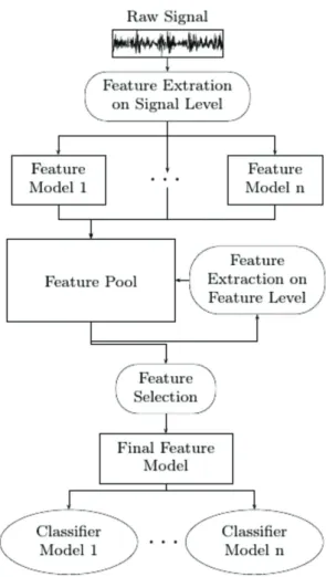
A generic framework for automatic fault diagnosis is presented in Figure 1. In this fig-ure, the first stage of the development is the raw signal acquisition. The present work uses the Case Western Reserve University Bearing Data Center as raw signal (CWRU, 2014). In the feature extraction at the signal level three feature extraction methods were used, statis-tical in time and frequency domain, wavelet package analysis and complex envelope spec-trum, grouped in a pool of features. No fea-ture extraction at the feafea-tures level was made. The feature selection can improve the classifier algorithms in performance and quality simul-taneously. Currently, several feature selection algorithms have been proposed, not only to improve quality and performance, but mainly
A fast feature selection algorithm applied to automatic
faults diagnosis of rotating machinery
Francisco de Assis Boldt, Thomas Walter Rauber, Flávio Miguel Varejão Universidade Federal do Espírito Santo. Av. Fernando Ferrari, 514, 29075-910, Vitória, ES, Brazil. [email protected], [email protected], [email protected]
Abstract. This work presents a fast algorithm to reduce the number of features of a classification system increasing the performance without loss of quality. The experiments show that the proposed algorithm can reduce the number of features quickly as well as increase the quality of the predictions simultaneously. Three features extractions were used to generate the initial pool of features of the system. Comparative results of the proposed algorithm with the classical sequential forward selection algorithm are shown. Keywords: feature selection, feature extraction, fault diagnosis, rotating machinery, supervised learning.
Figure 1. Generic framework for automatic fault diagnosis.
to reduce the time of the selection (Bermejo et al., 2011; Yu and Liu, 2003; Hsu et al., 2011). The main goal of this work is to present a fast feature selection algorithm, which reduces the features of the system without loss of the so-lutions quality. The classifier model used was the K-Nearest Neighbor (K-NN) algorithm (Cover and Hart 1967).
The following sections explain raw data acquisition, feature extraction techniques, traditional feature selection methods, state of the art of feature selection methods, fast algorithm as innovation, comparative experi-ments and conclusions.
Raw data acquisition
This work uses vibrational signals acquired from several bearing situations. The Case West-ern Reserve University Bearing Data Center (CWRU 2014) was chosen due to its public-ity and qualpublic-ity. The database is organized as MATLAB/Octave processable vibration signal files, with all necessary parameters attached, which are needed to calculate the feature mod-els. The machine condition differs with respect to the fault severity, bearing manufacturer, motor load, sensor position and acquisition frequency and duration. Figure 2 shows the schematic setup of the workbench used for the fault diagnosis experiments: motor, torque en-coder, dynamometer. The three different posi-tions of the accelerometers are shown.
This dataset is composed of vibratory sig-nals of normal and fault bearings extracted from a 2 hp reliance electric motor. The faults were introduced at a specific position of the bearing, using an electro-discharging machin-ing with fault diameters of 0.007, 0.014, 0.021 and 0.028 inches. A dynamometer induced
loads of 0, 1, 2 and 3 hp, changing the shaft rotation from 1797 to 1720 rpm. One model of bearing was used on the drive end and an-other was used at the fan’s end. Three accel-erometers collected the vibratory data, placed on the drive’s end, fan’s end and the base of the motor. Only few data files contain the base plate data. So the signals collected by this ac-celerometer were not used in the experiments. Neither 0.0028 inch fault diameter signal files were used because they do not have any signal from the fan’s end.
As done in other works (Xia et al., 2012; Liu, 2012; Wu et al., 2012), the signals were split in several parts before the feature extraction, aiming at a better classification performance estimation. The signals were split in 15 parts. Preliminary experiments showed that this was the maximum possible division without con-siderable loss of accuracy. The amount of sam-ples acquired is 2295. The classes can identify if both bearings are normal (1); if the defective bearing is in drive’s end or in fan’s end (2); the location of the failure in the bearing, ball, in-ner race and outer race (3); the severity of the failure in 0.007, 0.014 and 0.021 inches (3); and the motor load, 0, 1, 2 or 3 hp (4). The number of classes is (1+2*3*3)*4 = 76.
Feature extraction
The signals collected from the machinery are not directly usable for diagnosis, so it is necessary to extract static features. As rep-resentative models we use those mainly ob-served in the considered literature, statistical features from the time and frequency domains, wavelet packet energy and complex envelope magnitudes. This feature extraction models are explained in the following subsections.
Statistical features
Usable information can be extracted from vibrational signals in the time domain ac-quired by accelerometers using statistical tech-niques. These statistical techniques can also be applied to the signals in the frequency domain using Fourier analysis to transform the original signal. As a representative set, this work uses those features used in Xia et al. (2012). The set is composed of ten features from the time do-main and three features from the Fourier trans-form generated frequency domain. As soon as the signal in two domains is available, the cal-culus has a very low computational cost.
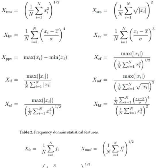
Table 1 presents the definition of statisti-cal features in the time domain as root mean
square (RMS), square root of the amplitude (SRA), kurtosis value (KV), skewness value (SV), peak-peak value (PPV), crest factor (CF), impulse factor (IF), margin factor (MF), shape factor (SF) and kurtosis factor (KF). Table 2 presents the definition of statistical features in the frequency domain as frequency center (FC), RMS frequency (RMSF) and root vari-ance frequency (RVF). Considering two bear-ings, drive end and fan end, the number of sta-tistical features is (10+3)*2 = 26.
Wavelet package analysis
Dual domain analysis methodologies that extract features from the time-frequency rep-resentation are represented in this work by
Table 1. Time domain statistical features.
wavelets (Gao and Yan, 2011). Posterior to the classical wavelet decomposition, the set of vi-bration analysis techniques has been enriched by the wavelet packet analysis (Coifman and Wickerhauser, 1992), which allows a more flexible decomposition guided by informa-tion theory. Work describing the CWRU data by wavelet packets is found in Chebil et al. (2009), Wei et al. (2011), Xia et al. (2012), Luo et al. (2013) and Liu (2012). For each purpose the wavelet family, the mother wavelet within this family and the decomposition depth have to be chosen. This work follows the procedure proposed in Xia et al. (2012), which uses as the mother wavelet Daubechies 4 and refining is done down to the fourth decomposition level. An application to rotating machinery with an extended description on how to select the appropriate wavelet base is described in Liu (2005). However, it is not possible to modify the tree structure by optimization of the
infor-mation contents of the leave nodes since it is necessary to obtain corresponding feature vec-tors for each sample. This means that a tree structure optimization for a normal machine condition could generate a wavelet packet tree that is different from the tree generated by a faulty condition thus not permitting the direct comparison of the features.
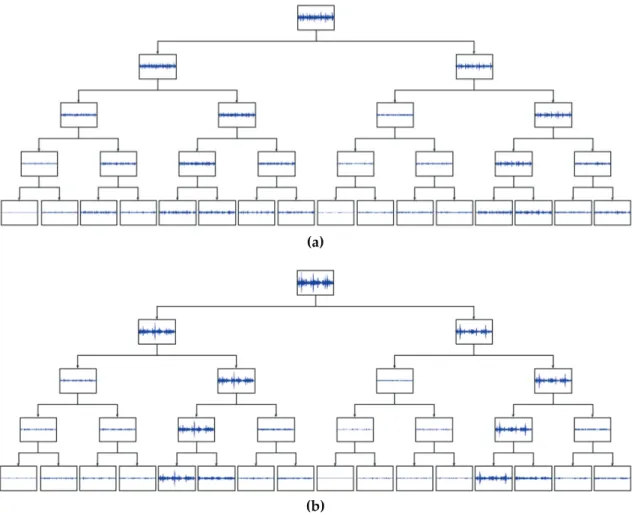
Figure 3 shows two comparative exam-ples extracted from real signals. Only the leaf nodes were used to calculate the features of two bearings. The total number of wavelet package analysis features is 16*2 = 32.
Complex envelope analysis
There are some frequency groups involved in a typical bearing fault. First there is the nat-ural high natnat-ural frequency (resonance) of the ball when hitting the defective region which can be located on itself, the cage, interior or
Figure 3. (a) 0.007 inch, 0 hp, inner race fault signal decomposition. (b) 0.021 inch, 3 hp, inner race fault signal decomposition. Wavelet packet tree of depth j = 4 for two inner race faults, varying with respect to the fault severity and work load. Only the first 0.1s of a single sample is processed and shown in order not to overburden the graph.
(a)
exterior raceway. Low frequencies are contrib-uted mainly by shaft rotation related faults, like unbalance or misalignment. It is necessary to establish a model of the bearing to under-stand these frequency groups.
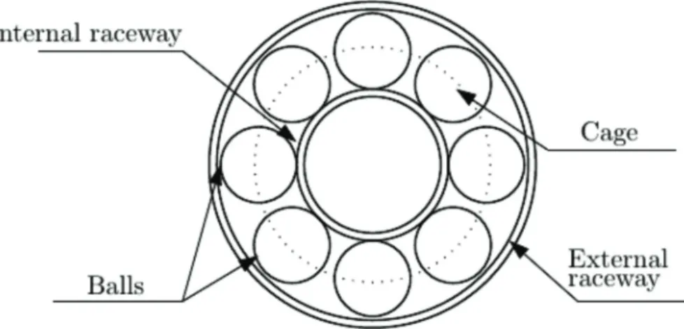
The structure of a rolling bearing allows to establish a model of possible faults. The bear-ings, when defective, present characteristic frequencies depending on the localization of the defect (Ragul’skis and Yurkauskas, 1989; Mobley, 1999; Rieger and Crofoot, 1977). There are four characteristic frequencies at which faults can occur. Knowing the shaft rotational frequency FS, the fault frequencies that can be calculated are the fundamental cage frequency FC, ball pass inner raceway frequency FBPI, ball pass outer raceway frequency FBPO and the ball spin frequency FB. For the ball bear-ings with angular contact with the cage, the outer ring is static and the inner ring rotates at the shaft speed. Figure 4 illustrates a basic model of a bearing with the rolling elements, the inner and outer raceways and the cage.
For the complex envelope analysis, first a high pass filter is applied in order to elimi-nate the influence of the low frequency vibra-tions caused by noise, unbalance and mis-alignment. Subsequently, an analytical signal is calculated by applying the Hilbert trans-form to the original signal and adding it in quadrature to it. The magnitude of the Fouri-er transform of the analytical signal translates the characteristic bearing faults frequencies to the low frequency band. The final features are the narrow band energy around the ex-pected fault frequencies and their harmonics. Six harmonics were calculated for each of the two bearings considered.
This kind of feature extraction needs a spe-cific feature for each fault, because it tries to identify high energy where the faults mani-fest themselves. This work intends to identify three types of faults, ball, inner race and outer race, using six harmonics for two bearings. Considering that each bearing produces fea-tures to identify failures in the other one, be-cause they have different dimensions, the total number of complex envelope analysis features is 3*6*2*2 = 72.
Feature selection
When automatic diagnosis systems or any other classification task extract a large amount of features, feature selection techniques can improve the application in both performance and quality of the results. The performance increment occurs because the classifier needs less memory and processor power to be trained and to identify a class. The quality of the results is improved because it is possible that some redundant or irrelevant features were extracted on the feature extraction stage (Kudo and Sklansky, 2000; Guyon and Elisse-eff, 2003). A feature selection algorithm is basi-cally composed of a selection criterion and a search strategy. There are two main classes of feature selection techniques. The wrapper ap-proach in feature selection consists of taking the estimated performance of a classifier as the proper feature selection criterion. The perfor-mance criterion in the overwhelming part of past and contemporary work is the estimat-ed accuracy of the classifier. This means that those features during the search are labeled
as good, what minimizes the estimated error. The filter approach uses different criteria to judge a feature set or judge the performance of the classifier. Usually the benefit of a selec-tion filter is its speed, its drawback is a pos-sible inferior performance compared to that of a wrapper. Finding the best combination of features is a combinatorial problem and it is necessary to use heuristics when the number of features is large.
Sequential Forward Selection (SFS) (Guyon and Elisseeff, 2003) is a well known wrapper technique. It starts with an empty set. For each single feature, a criterion, like accuracy for in-stance, is calculated and this feature is ranked. The best ranked feature is added to the subset of features. After this initial step, each remain-ing feature is evaluated with the current set, ranked and the best one is chosen to be added to the set. This process is repeated until the desired number of features is achieved. This algorithm can be used with both wrapper and filter criterion.
The Greedy Random Feature Selection Al-gorithm
Recent works present algorithms faster than SFS (Bermejo et al., 2011; Yu and Liu, 2003; Hsu et al., 2011). These works commonly try to reduce the number of wrapper evaluations. The main goal is reducing the number of fea-tures without loss of quality. One approach is mixing filter and wrapper techniques (Berme-jo et al., 2011; Hsu et al., 2011). The algorithm present in this work is simple, faster, easy to implement even in a parallel version. The hy-pothesis of this work is that filter techniques do not necessarily represent a good strategy to make the preliminary selection, and a repeti-tive random choice can achieve good results. The experimental results show that a random algorithm can be applied without loss of quali-ty. The performances of the random algorithm and of the SFS were compared.
The Greedy Random Feature Selection Algo-rithm (GRFS), in its simplest form, initializes the feature subset with a random feature and evalu-ates it. After this initial step, the GRFS selects an-other feature, also randomly, adds this feature to the subset and evaluates it again. If evalua-tion does not improve, this feature is discarded. If it improves, the feature is added to the subset. In each interaction, one feature is chosen from the subset, also randomly, to be taken out of the subset, which is evaluated. If evaluation does not improve, this feature is re-added to the set, or else, it is permanently discarded.
To test this feature selection algorithm, ex-periments were made using K-Nearest Neigh-bor (K-NN) classifier with the 130 features extracted from CWRU bearing data by the ex-traction models presented. The parameter K was set to one. This classifier was chosen due to its simplicity and speed with the dataset used. The metric of quality was accuracy. As in Bermejo et al. 2011, 5 fold cross-validation was used in all experiments. The first experi-ment runs the K-NN ten times with all 130 features. The values found were average of 94.67%, minimum of 93.81%, maximum of 95.16% and standard deviation of 0.37%. The second experiment was running the GRFS ten times, and the accuracy found was an average of 96.60%, minimum of 94.94%, maximum of 97.38 % and standard deviation of 0.70%. The number of features was in average 26.6, minimum 21, maximum 34 and standard de-viation of 3.84. These experiments show that GRFS can reduce the number of the features without loss of accuracy, for this data. The worse accuracy of GRFS was higher than the average of the system with the complete pool of features.
A dangerous drawback of the GRFS is that when it removes a feature, that feature never comes back. To minimize that, a slight modi-fication was made in the GRFS. A parameter called chance was added, so each feature had chances to improve the features subset. Figure 5 shows the accuracy varying the number of chances and Figure 6 shows the number of features varying the number of chances. For each value of chance ten experiments were executed. As expected, the accuracy average tends to grow with the number of chances. On the other hand, the number of features did not grow much.
To compare the results of GRFS, ten ex-periments with SFS were made and the results are presented in Figure 7. This figure shows that the SFS needs approximately 50 features to achieve its higher average of accuracy, and did not achieve 98% in average. No execution of the GRFS used more than 45 features, the mean was never higher than 97% for number of chances greater than 2.
The GRFS is much faster than the SFS, so it is possible to run it several times and choose the best result. Based on this fact, another lit-tle modification was made, adding another parameter called repetition. This parameter sets how many times the previous form of the GRFS will execute, and then, the algorithm
will choose the best result. Experiments with 10 repetitions with the parameter chance set as one were made. The final results after ten ex-ecutions were in accuracy average of 97.55%, minimum of 96.82%, maximum of 97.91%, and standard deviation of 0.31%. In number of
features the final results were average of 24.6, minimum of 18, maximum of 35, and stand-ard deviation of 6.29. Comparing the number of features, these results are almost compat-ible with the SFS, but extremely faster to be achieve, even with ten repetitions.
Figure 5. Accuracy varying the number of chances.
Figure 6. Number of features varying the number of chances.
The final version of the GRFS is shown in Algorithm 1.
Conclusions
This work presented a fast feature selec-tion algorithm and showed comparative ex-periments for testing its practical utilization. The experiments were based on a generic framework for diagnosis system develop-ment. The raw signals were acquired from CWRU (2014) bearing data center. Three
models of feature extraction were used. The features extracted were combined in a pool of features. The GRFS algorithm presented proved capable of reducing the number of features improving the accuracy of whole system. The SFS algorithm needs the number of features as a parameter before its execution and has high cost to find the best number of features. The GRFS does not need the final number of features as a parameter and can achieve good results faster than the SFS when the number of features is compared.
The GRFS proved to be a useful algorithm and has no restrictions to be used as filter or wrapper approach. It can be used as a param-eter to compare the performance and quality of the results to test new methods of feature selection. It can also be used to generate ini-tial solutions (Bermejo et al., 2011) for more so-phisticated heuristics.
References
BERMEJO, P.; GÁMEZ, J.A.; PUERTA, J.M. 2011. A GRASP algorithm for fast hybrid (filter-wrapper) feature subset selection in high-dimensional datasets. Pattern Recognition Letters, 32(5):701-711. http://dx.doi.org/10.1016/j.patrec.2010.12.016 CHEBIL, J.; NOEL, G.; MESBAH, M.; DERICHE, M.
2009. Wavelet decomposition for the detection and diagnosis of faults in rolling element bea-rings. Jordan Journal of Mechanical and Industrial Engineering, 3(4):260-267.
COIFMAN, R.R.; WICKERHAUSER, M.V. 1992. En-tropy-based algorithms for best basis selection. In-formation Theory, IEEE Transactions on, 38 (2):713-718. http://dx.doi.org/10.1109/18.119732
COVER, T.; HART, P. 1967. Nearest neighbor pat-tern classification. Information Theory, IEEE Transactions on, 13(1):21–27.
CWRU. 2014. Case Western Reserve University, Bearing Data Center. Available at: http://cseg-roups.case.edu/bearingdatacenter/home. Ac-cessed on: June 1st, 2014.
GAO, R. X., YAN, R. 2011. Wavelets: Theory and appli-cations for manufacturing. London, Springer, 224 p. http://dx.doi.org/10.1007/978-1-4419-1545-0 GUYON, I.; ELISSEEFF, A. 2003. An introduction to
variable and feature selection. Journal of Machine Learning Research, 3:1157–1182.
HSU, H.H.; HSIEH, C.W.; LU, M.D. 2011. Hybrid fe-ature selection by combining filters and wrappers. Expert Systems with Applications, 38(7):8144-8150. http://dx.doi.org/10.1016/j.eswa.2010.12.156 KUDO, M.; SKLANSKY, J. 2000. Comparison of
algo-rithms that select features for pattern classifiers. Pat-tern Recognition33:25–41.
http://dx.doi.org/10.1016/S0031-3203(99)00041-2 LIU, B. 2005. Selection of wavelet packet basis for
rota-ting machinery fault diagnosis. Journal of Sound and Vibration, 284(3):567-582.
http://dx.doi.org/10.1016/j.jsv.2004.06.047
LIU, J. 2012. Shannon wavelet spectrum analysis on truncated vibration signals for machine incipient fault detection. Measurement Science and Technolo-gy, 23(5):055604.
http://dx.doi.org/10.1088/0957-0233/23/5/055604 LUO, J.; YU, D.; LIANG, M. 2013. A kurtosis-guided
adaptive demodulation technique for bearing fault de-tection based on tunable-Q wavelet transform. Mea-surement Science and Technology, 24(5):055009. http://dx.doi.org/10.1088/0957-0233/24/5/055009 MOBLEY, R.K. 1999. Root Cause Failure Analysis
(Plant Engineering Maintenance Series). Boston, Newnes, 308 p.
RAGULSKIS, K.; YURKAUSKAS, A. 1989. Vibration of bearings. Bristol, Hemisphere, 119 p.
RANDALL, R.B. 2011. Vibration-based condition moni-toring: industrial, aerospace and automotive appli-cations. Hoboken, John Wiley & Sons, 289 p. http://dx.doi.org/10.1002/9780470977668
RIEGER, N.F.; CROFOOT, J.F. 1977. Vibration of Ro-tationary Machinary. [s.l.], Rochester Institute of Technology, p. 69-77.
WANDEKOKEM, E.D.; MENDEL, E.; FABRIS, F.; VALENTIM, M.; BATISTA, R.J.; VAREJÃO, F.M.; RAUBER, T.W. 2011. Diagnosing multi-ple faults in oil rig motor pumps using support vector machine classifier ensembles. Integrated Computer-Aided Engineering, 18(1):61-74.
WEI, Z.; GAO, J.; ZHONG, X.; JIANG, Z.; MA, B. 2011. Incipient fault diagnosis of rolling element bearing based on wavelet packet transform and energy operator. WSEAS TRANSACTIONS on SYSTEMS, 10(3):81-90.
WU, S.-D.; WU, P.-H.; WU, C.-W.; DING, J.-J.; WANG, C.-C. 2012. Bearing fault diagnosis based on multis-cale permutation entropy and support vector machi-ne. Entropy, 14(8):1343–1356.
http://dx.doi.org/10.3390/e14081343
XIA, Z.; XIA, S.; WAN, L.; CAI, S. 2012. Spectral re-gression based fault feature extraction for bearing ac-celerometer sensor signals. Sensors, 12(10):13694– 13719. http://dx.doi.org/10.3390/s121013694 YU, L., LIU, H. 2003. Feature selection for
high-di-mensional data: A fast correlation-based filter solution. ICML, 3:856-863.
Submitted on January 6, 2014 Accepted on June 11, 2014