Abstract—High-speed networks with large delays present a unique environment where TCP may have a problem utilizing the full bandwidth. Several congestion control proposals have been suggested to remedy this problem. The protocols consider mainly two properties: TCP friendliness and bandwidth scalability. That is, a protocol should not take away too much bandwidth from TCP while utilizing the full bandwidth of high-speed networks. This paper presents another important constraint, namely, RTT (round trip time) unfairness where competing flows with different RTTs may consume vastly unfair bandwidth shares. Existing schemes have a severe RTT unfairness problem because the window increase rate gets larger as window grows – ironically the very reason that makes them more scalable. RTT unfairness for high speed networks occurs distinctly with drop tail routers where packet loss can be highly synchronized. After recognizing the RTT unfairness problem of existing protocols, this paper presents a new congestion control protocol that ensures linear RTT fairness under large windows while offering both scalability and TCP-friendliness. The protocol combines two schemes called additive increase and binary search increase. When the congestion window is large, additive increase with a large increment ensures linear RTT fairness as well as good scalability. Under small congestion windows, binary search increase is designed to provide TCP friendliness. The paper presents a performance study of the new protocol.
Key words – Congestion control, High speed networks, RTT fairness, TCP friendliness, Scalability, Simulation, Protocol Design.
I. INTRODUCTION
he Internet is evolving. The networks, such as Abilene and ESNet, provisioned with a large amount of bandwidth ranging from 1 to 10Gbps are now sprawling to connect many research organizations around the world. As these networks run over a long distance, their round trip delays can rise beyond 200ms.
The deployment of high-speed networks has helped push the frontiers of high performance computing that requires access to a vast amount of data as well as high computing power. Applications like scientific collaboration, telemedicine, and real-time environment monitoring benefit from this deployment. Typically they require transmission of high-bandwidth real time data, images, and video captured from remote sensors such as 1 Authors are with the Department of Computer Science, North Carolina
State University, Raleigh, NC 27699 (email: lxu2@cs.ncsu.edu,
Harfoush@cs.ncsu.edu, rhee@cs.ncsu.edu). The work reported in this paper is sponsored in part by NSF CAREER ANI-9875651, NSF ANI-0074012
satellite, radars, and echocardiography. These applications require not only high bandwidth, but also real time predictable, low latency data transfer.
TCP has been widely adopted as a data transfer protocol for these networks. However, it is reported [1, 2, 4, 7] that TCP substantially underutilizes network bandwidth over high-speed connections. TCP increases its congestion window by one at every round trip time (RTT) and reduces it by half at a loss event. In order for TCP to increase its window for full utilization of 10Gbps with 1500-byte packets, it requires over 83,333 RTTs. With 100ms RTT, it takes approximately 1.5 hours, and for full utilization in steady state, the loss rate cannot be more than 1 loss event per 5,000,000,000 packets which is less than the theoretical limit of the network’s bit error rates.
Fine-tuning TCP parameters such as receiver windows and network interface buffers [9, 10, 11, 12] may mitigate this problem. One straightforward solution is to increase the packet size by using the Jumbo packet option (up to 8KB) and use multiple TCP connections [13, 14, 15]. Although these approaches enhance utilization, they do not ensure TCP friendliness when running in the TCP’s “well-behaving” operating range (between loss rates of 10-2 to 10-4) because the window increase rate is fixed to
be always larger than TCP. Guaranteeing both TCP friendliness and bandwidth scalability with one fixed increase rate of window is challenging. It calls for adaptive schemes that vary the window growth rate depending on network conditions.
After recognizing TCP’s limitation, the networking research community responded quickly. Several promising new protocols have been put forward: High Speed TCP (HSTCP) [1, 2, 3], Scalable TCP (STCP) [4], FAST [7], XCP [5], and SABUL [6]. Except XCP (a router assisted protocol), these protocols adaptively adjust their increase rates based on the current window size. So the larger the congestion window is, the faster it grows. These protocols are claimed to be TCP friendly under high loss rate environments as well as highly scalable under low loss environments.
In this paper, we evaluate some of these protocols, in particular, window-based, self-clocking protocols known for safer incremental deployment [16]. We don’t consider SABUL because it is a rate-based protocol. Further, since
Binary Increase Congestion Control for Fast,
Long Distance Networks
Lisong Xu, Khaled Harfoush, and Injong Rhee1
the detailed description of FAST is not yet available, we consider only HSTCP and STCP in this paper.
Our study reveals that notwithstanding their scalability and TCP friendliness properties, HSTCP and STCP have a serious RTT unfairness problem when multiple flows with different RTT delays are competing for the same bottleneck bandwidth. We define the RTT unfairness of two competing flows to be the ratio of windows in terms of their RTT ratio.2 Under a completely synchronized loss
model, STCP does not even find a convergence point such that shorter RTT flows eventually starve off longer RTT flows. We also find that in HSTCP, two flows with RTT1 and RTT2 has RTT unfairness in proportion to
(
RTT2 RTT1)
4.56. This problem commonly appearsfor drop tail routers while the severity reduces for RED, and therefore, greatly impairs the ability to incrementally deploy the protocols, without adequate support from active queue management (such as RED and XCP).
RTT unfairness stems from the adaptability of these protocols – ironically the very reason that makes them more scalable to large bandwidth; in these protocols, a larger window increases faster than a smaller window. Compounded with a delay difference, RTT unfairness gets worse as the window of a shorter RTT flow grows faster than that of a longer RTT flow.
Another source of the problem is synchronized loss
where packet loss occurs across multiple competing flows simultaneously. When the congestion window gets larger, the probability that a window loses at least one packet (i.e., loss event) increases exponentially. Assuming uniform distribution of random loss probability p, the probability of a loss event is (1- (1- ) )p w . Even a small packet loss
rate at a router can cause loss events across multiple flows of large windows. Although a long-term packet loss rate could be low in high-speed connections, a short-term loss rate during the period when packet loss occurs (due to buffer overflow) can be high.
Synchronized loss encourages RTT unfairness; since loss events are more uniform across different window sizes if the size is larger than a certain limit, large windows with a short RTT can always grow faster than small windows with a long RTT. Furthermore, synchronization can prolong convergence and cause a long-term oscillation of data rates, thereby hurting fairness in short-term scales. In our simulation, we observe the short-term unfairness of STCP and HSTCP over both drop-tail and RED routers.
It is challenging to design a protocol that can scale up to 10Gbps in a reasonable range of loss rates (from 10-7 to
10-8); at the same time, can be RTT fair for the large
2 RTT unfairness is often defined in terms of the ratio of throughout. The
window ratio can be converted into throughput ratio by multiplying one RTT ratio to the window ratio.
window regime where synchronized loss can occur more frequently; and is TCP friendly for higher loss rates (between 10-1 to 10-3). For instance, while AIMD can
scale its bandwidth share by increasing its additive increase factor, and also provide linear RTT fairness, it is not TCP friendly. HSTCP and STCP are extremely scalable under low loss rates and TCP friendly under high loss rates. But they are not RTT fair.
In this paper, we consider a new protocol that may satisfy all these criteria, called Binary Increase TCP
(BI-TCP). BI-TCP has the following features:
1. Scalability: it can scale its bandwidth share to 10 Gbps around 3.5e-8 loss rates (comparable to HSTCP which reaches 10Gbps at 1e-7).
2. RTT fairness: for large windows, its RTT unfairness is proportional to the RTT ratio as in AIMD.
3. TCP friendliness: it achieves a bounded TCP fairness for all window sizes. Around high loss rates where TCP performs well, its TCP friendliness is comparable to STCP’s.
4. Fairness and convergence: compared to HSTCP and STCP, it achieves better bandwidth fairness over various time scales and faster convergence to a fair share.
This paper reports a performance study of BI-TCP. The paper organized as follows: Section II describes our simulation setup and Section III discusses evidence for synchronized loss. In Sections IV and V, we discuss the behavior of HSTCP and STCP. In Section VI, we describe BI-TCP and its properties. Section VII gives details on simulation results. Related work and conclusion can be found in Sections VIII and IX.
II. SIMULATION SETUP
Fig. 1 shows the NS simulation setup that we use throughout the paper. Various bottleneck capacity and delays are tested. The buffer space at the bottleneck router is set to 100% of the bandwidth and delay products of the bottleneck link. Every traffic passes through the
N1 N2 Bottleneck Link forward S1 S2 Sn backward D1 D2 S3 D3 Dn
Fig. 1. Simulation network topology
xms
bottleneck link; each link is configured to have different RTTs and different starting times and end times to reduce the phase effect [17]. A significant amount of web traffic (20% up to 50% of bottleneck bandwidth when no other flows are present) is generated both for both directions to remove synchronization in feedback. 25 small TCP flows with their congestion window size limited to be under 64 are added in both directions whose starting and finishing times are set randomly. Two to four long-lived TCP flows are created for both directions. The background traffic (long-lived TCP, small TCP flows, and web traffic) consumes at the minimum 20% of the backward bandwidth.
The simulation topology does not deviate too much from that of the real high-speed networks. High-speed networks of our interest are different from the general Internet where a majority of bottlenecks are located at the edges. In the high-speed networks, edges can still be high-speed and the bottleneck could be at the locations where much high-speed traffic meets such as Startlight in Chicago that connects CERN (Geneva) and Abilene.
We make no claim about how realistic our background traffic is. However, we believe that the amount of background traffic in both directions, and randomized RTTs and starting and finishing times are sufficient to reduce the phase effect and synchronized feedback. We also paced TCP packets so that no more than two packets are sent in burst. A random delay between packet transmissions is inserted to avoid the phase effect
(overhead = 0.000008).We test both RED and drop tail
routers at the bottleneck link. For RED, we use adaptive RED with the bottom of max_p set to 0.001.3
III. SYNCHRONIZED PACKET LOSS
In this paper, we use a synchronized loss model for the analysis of RTT fairness. Before delving into the analysis, we provide some evidence that synchronized loss can happen quite frequently in high speed networks.
To measure the extent of synchronization, we run a simulation experiment involving 20 high-speed connections of HSTCP with RTTs varying from 40ms to 150ms. The bottleneck bandwidth is 2.5Gbps. Background traffic takes about 7% of the forward path bandwidth and about 35% of the backward path bandwidth. The reason why the forward path background traffic takes less bandwidth is that the forward path high-speed connections steal the bandwidth from the TCP connections. We define a loss epoch to be one-second period that contains at least one loss event by a high-speed flow. We count the number of unique high-speed flows that have at least one loss event in the same epoch, and 3 It is recommended by [1] to reduce synchronized loss – normally this value
is set to 0.01.
then add the number of epochs that have the same number of flows.
Figure 2 shows the accumulative percentage of loss epochs that contain at the minimum a given number of high-speed flows. In drop tail, the percentage of loss epochs that involve more than half of the total high-speed flows (20 in this experiment) is around 70%. This implies that whenever a flow has a loss event in the drop tail router, the probability that at least half of the total flows experience loss events at the same time is around 70%. On the other hand, RED does not incur as much synchronized loss. However, there still exists some amount of synchronization; the probability that more than a quarter of the total flows have synchronized loss events is around 30%.
Fig. 2: Accumulative percentage of loss epoch containing at least a given number of unique flows.
0 10 20 30 40 50 60 70 80 90 100 1 4 7 10 13 16 19 Number of flows Pe rc en ta ge of los s e poc h DROP TAIL RED
The result implies that the number of synchronized loss can be quite substantial in drop tail. Although it requires real network tests to confirm this finding, we believe that our simulation result is not difficult to recreate in real networks. We leave that to future study. Synchronized loss has several detrimental effects such as RTT unfairness, slower convergence, under-utilization, and degraded fairness.
IV.RTTFAIRNESS OF HSTCP AND STCP
In this section, we analyze the effect of synchronized loss on the RTT fairness of HSTCP and STCP. We use a synchronized loss model where all high-speed flows competing on a bottleneck link experience loss events at the same time. By no means, we claim that this model characterizes all the aspects of high-speed networks. We use this model to study the effect of synchronized loss on RTT unfairness and to gain insight to RTT unfairness we observe in our simulation experiment.
Let wi and RTTi denote the window size just before a loss event and the RTT of flow i (i=1, 2) respectively. Let
t denote the interval between two consecutive loss events during steady state.
HSTCP employs an additive increase and multiplicative decrease window control protocol, but their increase and decrease factors α and β are functions of window size. 1 1 1 1 1 2 2 2 2 2 (1 ( )) ( ) (1 ( )) ( ) t w w w w RTT t w w w w RTT β α β α = − + = − + By substituting 2 2 ( ) ( ) ( ) 2 ( ) w w p w w w β α β = − , and 0.82 0.15 ( ) w p w =
which is given by [1], we get
56 . 4 1 2 1 2 2 1 ) ( 2 ) ( 2 − − = RTT RTT w w w w
β
β
STCP uses multiplicative increase and multiplicative decrease (MIMD) with factors α and β.
1 2 1 1 2 2 (1 )(1 ) (1 )(1 ) t RTT t RTT w w w w
β
α
β
α
= − + = − + The above equations do not have a solution. That is, there is no convergence point for STCP. The shorter RTT flow consumes all the bandwidth while the longer RTT flow drops down to zero.
Table 1 presents a simulation result that shows the bandwidth shares of two high-speed flows with different ratios of RTTs running in drop tail (RED does not show significant RTT unfairness). The ratio of RTTs is varied to be 1 to 6 with base RTT 40ms.
AIMD shows a quadratic increase in the throughput ratio as the RTT ratio increases (i.e., linear RTT unfairness). STCP shows over 300 times throughput ratio for RTT ratio 6. HSTCP shows about 131 times throughput ratio for RTT ratio 6. Clearly the results indicate extremely unfair use of bandwidth by a short RTT flow in drop tail.
The result shows better RTT unfairness than predicted by the analysis. This is because while the analysis is based on a completely synchronized loss model, the simulation may involve loss events that are not synchronized. Also when the window size becomes less than 500, the
occurrence of synchronized loss is substantially low. Long RTT flows continue to reduce their windows up to a limit where synchronized loss does not occur much. Thus, the window ratio does not get worse.
Figure 3 shows a sample simulation run with ten STCP flows in drop tail. All flows are started at different times. Eight flows have 80 ms RTT, and two flows have 160 ms RTT. It exhibits a typical case of RTT unfairness. The two longer RTT flows slowly reduce their window down to almost zero while the other flows merge into a single point. Note that STCP does not converge in a completely synchronized model because of MIMD window control [20]. However, in this simulation, 8 flows with the same RTT do converge (despite high oscillation). This indicates that there exists enough asynchrony in packet loss to make the same RTT flows converge, but not enough to correct RTT unfairness.
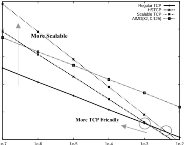
V. RESPONSE FUNCTION
The response function of a congestion control protocol is
its sending rate in a function of packet loss rate. It can give much information about the protocol, especially, its TCP friendliness, RTT fairness, convergence, and scalability. Figure 4 draws the response functions of HSTCP, STCP, AIMD, and TCP in a log-log scale. AIMD uses the increase factor 32 and the decrease factor 0.125.
It can be shown that for a protocol with a response function c p/ dwhere c and d are constants, and p is a loss event rate, RTT unfairness is roughly proportional to
/(1 )
2 1
(RTT RTT/ )d −d
[8]. The values for TCP, AIMD, HSTCP, and STCP are 0.5, 0.5, 0.82, and 1, respectively. As d increases, the slope of the response function and RTT unfairness increase. A slope of a response function in a log-log scale determines its RTT unfairness. Since TCP and AIMD have the same slope, the RTT unfairness of AIMD is the same as TCP – linear RTT unfairness. The RTT unfairness of STCP is infinite while that of HSTCP
0 2000 4000 6000 8000 10000 12000 14000 16000 18000 20000 0 50 100 150 200 250 300 350 400 450
Window Size (packets/RTT))
Time (sec) STCP0 STCP1 STCP2 STCP3 STCP4 STCP5 STCP6 STCP7 STCP8 STCP9
Fig. 3: 10 scalable TCP flows; 2.4 Gbps, Drop tail.
RTT Ratio 1 3 6
AIMD 1.05 6.56 22.55
HSTCP 0.99 47.42 131.03
STCP 0.92 140.52 300.32
Table 1: The throughput ratio of two high speed flows over various RTT ratios in 2.5Gbps networks.
falls somewhere between TCP’s and STCP’s. Any slope higher than STCP would get infinite RTT unfairness.
The TCP friendliness of a protocol can be inferred by the point where the response function of the protocol crosses that of TCP. HSTCP and STCP work the same as the normal TCP operation below the point where their response functions cross TCP’s. Since TCP does not consume all the bandwidth at lower loss rates, a scalable protocol does not have to follow TCP over lower loss rates. Above the point, HSTCP and STCP run their own “scalable” protocols, ideally consuming what’s left by TCP flows. Under this strategy, it becomes more TCP friendly if a protocol crosses TCP as low a loss rate as possible (to the left of the X axis) since the protocol follows TCP below that point. However, moving the cross point to the left increases the slope of the response function if scalability has to be maintained at the same time, hurting RTT fairness.
An ideal protocol would be that (1) its response function crosses TCP’s as low a rate as possible, and at the same time (2) under lower loss rates, its slope is as close as that of AIMD. Note that the function need not be a straight line, i.e., the slope can vary depending on loss rates. But its slope at any loss rates should not exceed that of STCP although it can be much more forgiving under a high loss rate where window size is small enough to avoid frequent synchronized loss.
VI. BINARY INCREASE CONGESTION CONTROL.
It is challenging to design a protocol that can satisfy all three criteria: RTT fairness, TCP friendliness, and scalability. As noted in Section V, these criteria may not be satisfied simultaneously for all loss rates. A protocol should adapt its window control depending on the size of windows. Below, we present such a protocol, called
Binary Increase TCP (BI-TCP). BI-TCP consists of two
parts: binary search increase and additive increase. Binary search increase: We view congestion control as a searching problem in which the system can give yes/no feedback through packet loss as to whether the current sending rate (or window) is larger than the network capacity. The currentminimum window can be estimated as the window size at which the flow does not see any packet loss. If the maximum window size is known, we can apply a binary search technique to set the target window size to the midpoint of the maximum and minimum. As increasing to the target, if it gives any packet loss, the current window can be treated as a new maximum and the reduced window size after the packet loss can be the new minimum. The midpoint between these new values becomes a new target.
The rationale for this approach is that since the network incurs loss around the new maximum but did not do so around the new minimum, the target window size must be in the middle of the two values. After reaching the target and if it gives no packet loss, then the current window size becomes a new minimum, and a new target is calculated. This process is repeated with the updated minimum and maximum until the difference between the maximum and the minimum falls below a preset threshold, called the
minimum increment (Smin). We call this technique binary
search increase.
Binary search increase allows bandwidth probing to be more aggressive initially when the difference from the current window size to the target window size is large, and become less aggressive as the current window size gets closer to the target window size. A unique feature of the protocol is that its increase function is logarithmic; it reduces its increase rate as the window size gets closer to the saturation point. The other scalable protocols tend to increase its rates so that the increment at the saturation point is the maximum in the current epoch (defined to be a period between two consecutive loss events). Typically, the number of lost packets is proportional to the size of the last increment before the loss. Thus binary search increase can reduce packet loss. As we shall see, the main benefit of binary search is that it gives a concave response function, which meshes well with that of additive increase described below. We discuss the response function of BI-TCP in Section VI-B.
Additive Increase: In order to ensure faster convergence and RTT-fairness, we combine binary search increase with an additive increase strategy. When the distance to the midpoint from the current minimum is too large, increasing the window size directly to that midpoint might add too much stress to the network. When the distance from the current window size to the target in binary search increase is larger than a prescribed maximum step, called the maximum increment (Smax)
1e+1 1e+2 1e+3 1e+4 1e+5 1e+6
1e-7 1e-6 1e-5 1e-4 1e-3 1e-2
Sending Rate R (Packet/RTT)
Loss Event Rate Pevent
Regular TCP HSTCP Scalable TCP AIMD(32, 0.125) More Scalable More TCP Friendly
instead of increasing window directly to that midpoint in the next RTT, we increase it by Smax until the distance becomes less than Smax, at which time window increases directly to the target. Thus, after a large window reduction, the strategy initially increases the window linearly, and then increases logarithmically. We call this combination of binary search increase and additive increase binary increase.
Combined with a multiplicative decrease strategy, binary increase becomes close to pure additive increase under large windows. This is because a larger window results in a larger reduction by multiplicative decrease, and therefore, a longer additive increase period. When the window size is small, it becomes close to pure binary search increase – a shorter additive increase period.
Slow Start: After the window grows past the current maximum, the maximum is unknown. At this time, binary search sets its maximum to be a default maximum (a large constant) and the current window size to be the minimum. So the target midpoint can be very far. According to binary increase, if the target midpoint is very large, it increases linearly by the maximum increment. Instead, we run a “slow start” strategy to probe for a new maximum up to Smax. So if cwnd is the current window and the maximum increment is Smax, then it increases in each RTT round in steps cwnd+1, cwnd+2, cwnd+4,…, cwnd+Smax. The rationale is that since it is likely to be at the saturation point and also the maximum is unknown, it probes for available bandwidth in a “slow start” until it is safe to increase the window by Smax. After slow start, it switches
to binary increase.
Fast convergence: It can be shown that under a completely synchronized loss model, binary search increase combined with multiplicative decrease converges to a fair share [8]. Suppose there are two flows with different window sizes, but with the same RTT. Since the larger window reduces more in multiplicative decrease (with a fixed factor β), the time to reach the target is longer for a larger window. However, its convergence time can be very long. In binary search increase, it takes log(d)-log(Smin) RTT rounds to reach the maximum window after a window reduction of d. Since the window increases in a log step, the larger window and smaller window can reach back to their respective maxima very fast almost at the same time (although the smaller window flow gets to its maximum slightly faster). Thus, the smaller window flow ends up taking away only a small amount of bandwidth from the larger flow before the next window reduction. To remedy this behavior, we modify the binary search increase as follows.
In binary search increase, after a window reduction, new maximum and minimum are set. Suppose these values are max_wini and min_wini for flow i (i=1, 2). If the new maximum is less than the previous, this window is in
a downward trend (so likely to have a window larger than the fair share). Then, we readjust the new maximum to be the same as the new target window (i.e.,
max_wini=(max_wini-min_wini)/2), and then readjust the
target. After then we apply the normal binary increase. We call this strategy fast convergence.
Suppose that flow 1 has a window twice as large as flow 2. Since the window increases in a log step, convergent search (reducing the maximum of the larger window by half) allows the two flows to reach their maxima approximately at the same time; after passing their maxima, both flows go into slow start and then additive increase, during which their increase rates are the same and they equally share bandwidth of
max_win1-(max_win1-min_win1)/2. This allows the two
flows to converge faster than pure binary increase. Figure 5 shows a sample run of two BI-TCP flows. Their operating modes are marked by circles and arrows.
A. Protocol Implementation
Below, we present the pseudo-code of BI-TCP implemented in TCP-SACK.
The following preset parameters are used:
low_window: if the window size is larger than this
threshold, BI-TCP engages; otherwise normal TCP increase/decrease.
Smax: the maximum increment.
Smin: the minimum increment.
β: multiplicative window decrease factor.
default_max_win: default maximum (a large integer)
The following variables are used:
max_win: the maximum window size; initially default maximum.
min_win: the minimum window size
prev_win: the maximum window just before the current
maximum is set. 0 100 200 300 400 500 600 700 0 10 20 30 40 50 60 Window (packets/RTT) Time (sec) Binary Increase, Drop Tail
BI-TCP0 BI-TCP1 Binary Search Increase
Fast convergence
Slow start Additive
Increase
target_win: the midpoint between maximum and minimum
cwnd: congestion window size;
is_BITCP_ss: Boolean indicating whether the protocol is
in the slow start. Initially false.
ss_cwnd: a variable to keep track of cwnd increase
during the BI-TCP slow start.
ss_target: the value of cwnd after one RTT in BI-TCP
slow start. When entering faster recovery:
if (low_window <= cwnd){
prev_max = max_win;
max_win = cwnd;
cwnd = cwnd * (1-β);
min_win = cwnd;
if (prev_max > max_win) //Fast. Conv.
max_win = (max_win + min_win)/2;
target_win = (max_win + min_win)/2;
} else {
cwnd = cwnd *0.5; // normal TCP }
When not in fast recovery and an acknowledgment for a new packet arrives:
if (low_window > cwnd){
cwnd = cwnd + 1/cwnd; // normal TCP
return
}
if (is_BITCP_ss is false){// bin. increase
if (target_win – cwnd < Smax)// bin.
search
cwnd += (target_win-cwnd)/cwnd;
else
cwnd += Smax/cwnd; // additive incre.
if (max_win > cwnd){
min_win = cwnd;
target_win =(max_win+min_win)/2;
} else { is_BITCP_ss = true; ss_cwnd = 1; ss_target = cwnd+1; max_win = default_max_win; }
} else { // slow start
cwnd = cwnd + ss_cwnd/cwnd; if(cwnd >= ss_target){ ss_cwnd = 2*ss_cwnd; ss_target = cwnd+ss_cwnd; } if(ss_cwnd >= Smax) is_BITCP_ss = false; } B. Characteristics of BI-TCP
In this section, we analyze the response function and RTT fairness of BI-TCP. An analysis on the convergence and smoothness of the protocol can be found in [8].
1) Response function of BI-TCP
In this section, we present a deterministic analysis on the response function of BI-TCP.
We assume that a loss event happens at every 1/p
packets. We define a congestion epoch to be the time period between two consecutive loss events. Let Wmax denote the window size just before a loss event. After a loss event, the window size decreases to Wmax(1-β).
BI-TCP switches from additive increase to binary search increase when the distance from the current window size to the target window is less than Smax. Since the target window is the midpoint between Wmax and the current window size, it can be said that BI-TCP switches between those two increases when the distance from the current window size to Wmax is less than 2Smax. Let N1 and
N2 be the numbers of RTT rounds of additive increase and binary search increase, respectively. We have
) 0 , 2 max( 1 − = max max S W N
β
Then the total amount of window increase during binary search increase can be expressed as Wmaxβ-N1Smax. Assuming that this quantity is divisible by Smin, then N2 can be obtained as follows.
2 log 1 2 2 + − = min max max S S N W N
β
During additive increase, the window grows linearly with slope 1/Smax. So, the total number of packets during additive increase, Y1, can be obtained as follows.
1
1 1
1
( (1 ) (1 ) ( 1) )
2 max max max
Y = W −β +W −β + N − S N (1.1) During binary search increase, the window grows logarithmically. So, the total number of packets during binary search increase, Y2, can be expressed as follows.
min max max NS S W N W Y2 = max 2−2(
β
− 1 )+ (1.2) The total number of RTTs in an epoch is N = N1+ N2,and the total number of packets in an epoch is Y = Y1 + Y2. Since a loss event happens at every 1/p packets, Y can be expressed as follows: Y = 1/p. Solving it using Eqns. (1.1) and (1.2), we may express Wmax as a function of p. Below, we give the closed-form expression of Wmax for two special cases.
First, we assume that Wmaxβ > 2Smax, and Wmaxβ is divisible by Smax. Then N1= Wmaxβ/Smax -2. Now we can get
2 4 ( 1) 2 max b b a c p W a − + + + =
where a = β (2-β)/(2Smax), b = log2(Smax/Smin)+(2-β)/2, and c = Smax - Smin. The average sending rate, R, is then given as follows. 2 1 (2 ) 1 (2 ) 4 ( ) (1 ) 2 Y p R N b a c b p β β β β − = = − + + + − + (1.3)
In case that Wmaxβ>> 2Smax, for a fixed Smin, N1>>N2. Therefore, the sending rate of BI-TCP mainly depends on the linear increase part, and for small values of p, the sending rate can be approximated as follows:
2 1 2 max S R p β β −
≈ when Wmaxβ>> Smax (1.4) Note that for a very large window, the sending rate becomes independent of Smin. Eqn. (1.4) is very similar to the response function of AIMD [18] denoted as follows.
2 1 2 AIMD R p α β β − ≈
For a very large window, the sending rate of BI-TCP is close to the sending rate of AIMD with increase parameter α = Smax
Next, we consider the case when Wmaxβ ≤ 2Smax, then
N1=0, Assuming 1/p>>Smin, we get Wmax as follows.
max max 2 min 1 log 2(1 ) W W p S β β ≈ + −
By solving the above equation using function
LambertW(y) [21], which is the only real solution of
x
x e⋅ = y, we can get a closed-form expression for Wmax.
2 ln( 2) ln(2) 4 ln(2) max min W e LambertW p pS β β − = then, max max max 2 2 min min 1 2 1 log 2 log 2 Y p R W W W N S S β β β = = ≈ − + +
When 2β <<log(Wmaxβ/ Smin)+2, max
W
R≈ (1.5)
Note that when Wmaxβ≤ 2Smax, the sending rate becomes independent of Smax.
In summary, the sending rate of BI-TCP is proportional to 1/pd, with 1/2 < d <1. As the window size increases, d decreases from 1 to 1/2. For a fixed β, when the window size is small, the sending rate is a function of Smin and, when the window size is large, a function of Smax. Our objective is that when window is small, the protocol is TCP-friendly, and when the window is large, it is more RTT fair and gives a higher sending rate than TCP. We can now achieve this objective by adjusting Smin and Smax. Before we give details on how to set these parameters, let us examine the RTT fairness of BI-TCP.
2) RTT fairness of BI-TCP
As in Section IV, we consider the RTT fairness of a protocol under the synchronized loss model. Suppose
RTTi be the RTT of flow i (i=1,2). Let wi denote Wmax of flow i, and ni denote the number of RTT rounds in a congestion epoch of flow i. As described in the previous section, ni is a function of wi. Let t denote the length of an epoch during steady state. Since both flows have the same epoch, we have = = t RTT n t RTT n 2 2 1 1
Solving the above equations, we can express w1/w2 as a
function of RTT2/RTT1. As before, we consider special
cases to get a closed-form expression.
First, when Wmaxβ > 2Smax, we can obtain w1/w2 as
follows. 2 1 1 2 2 2 2 1 1 1 log ( ) 1 1 log ( ) max min max min S RTT t S w S w RTT t S RTT RTT − = − ≈ when t is large. Next, when Wmaxβ≤ 2Smax, w1/w2 can be expressed as
follows. ) 2 ln( ) 2 1 1 1 ( 2 1 t RTT RTT e w w − =
Note that t increases with the total bandwidth. Therefore, as the total bandwidth increases, the ratio first exponentially increases reaching its peak when Wmaxβ= 2Smax, and then becomes roughly linearly proportional to
RTT2/RTT1. This exponential RTT fairness can be problematic under larger windows. However, since under small windows, synchronized loss is less frequent, we believe that this unfairness can be managed to be low. We verify this in Section VII.
In this section, we discuss a guideline to determine the preset parameters of BI-TCP: β, Smin, Smax and
low_window in Section VI-A.
From Eqns.(1.4) and (1.5), we observe that reducing β increases the sending rate. Reducing β also improves utilization. However it hurts convergence since larger window flows give up their bandwidth slowly. From the equations, we can infer that β has a much less impact on the sending rate than Smax. So it is easier to fix β and then adjust Smin and Smax. We choose 0.125 for β . Under steady state, this can give approximately 94% utilization of the network. STCP chooses the same value for β .
For a fixed β = 0.125, we plot the response function as we vary Smax and Smin. Figure 6 shows the response function for different values of Smax.As Smax increases, the sending rate increases only for low loss rates using 1e-4 as a pivot. Smax allows us to control the scalability of BI-TCP for large windows. We cannot increase Smax arbitrarily high since it effectively increases the area of RTT unfairness (the area where the slope is larger than TCP’s). Recall that when Wmaxβ≤ 2Smax, the protocol is less RTT fair. This area needs to be kept small to reduce the RTT unfairness of the protocol.
Figure 7 plots the response function for various values of Smin. As we reduce Smin, the sending rate reduces around high loss rates (i.e., small windows) and the cross point between TCP and BI-TCP moves toward a lower loss rate. Since we can set low_window to the window size at the point where the protocol switches from TCP to BI-TCP, reducing Smin improves TCP friendliness. However, we cannot reduce Smin arbitrarily low because it makes the slope of the response function steeper before merging into the linear growth area, worsening RTT unfairness. HSTCP crosses TCP at window size of 31, and STCP at 16.
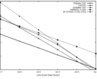
For a fixed β = 0.125, we plot the response function of BI-TCP with Smax = 32 and Smin = 0.01 in Figure 8. For comparison, we plot those of AIMD (α = 32, β = 0.125), HSTCP, STCP, and TCP. We observe that BI-TCP crosses TCP around p = 1e-2 and it also meets AIMD around p=1e-5 and stays with AIMD. Clearly, BI-TCP sets an upper bounds on TCP friendliness since the response functions of BI-TCP and TCP run in parallel after some point (at p=1e-5). BI-TCP’s TCP-friendliness under high loss rates is comparable to STCP’s, but less than HSTCP’s. BI-TCP crosses TCP at the window size of 14 (lower than STCP and HSTCP). The sending rate of BI-TCP over extremely low loss rates (1e-8) is less than that of STCP and HSTCP.
Smin
Fig 7: Response functions of BI-TCP for different values of Smin.
1 1e+1 1e+2 1e+3 1e+4 1e+5 1e+6 1e+7
1e-8 1e-7 1e-6 1e-5 1e-4 1e-3 1e-2 1e-1
Sending Rate R (Packet/RTT)
Loss Event Rate P BI-TCP Smax=32 beta=0.125
Regular TCP BI-TCP with Smin=1 BI-TCP with Smin=0.1 BI-TCP with Smin=0.01 BI-TCP with Smin=0.001 1 1e+1 1e+2 1e+3 1e+4 1e+5 1e+6 1e+7
1e-8 1e-7 1e-6 1e-5 1e-4 1e-3 1e-2 1e-1
Sending Rate R (Packet/RTT)
Loss Event Rate P BI-TCP Smin=0.01 beta=0.125
Regular TCP BI-TCP with Smax=8 BI-TCP with Smax=16 BI-TCP with Smax=32 BI-TCP with Smax=64
Fig. 6: Response functions of BI-TCP for different values of Smax. Smax
Linear Growth
VII. EXPERIMENTAL STUDY
In this section, we compare the performance of BI-TCP using simulation with that of HSTCP, STCP, and AIMD. Every experiment uses the same simulation setup described in Section II. Unless explicitly stated, the same amount of background traffic is used for all the experimental runs. In order to remove noise in data sampling, we take measurement only in the second half of each run. We evaluate BI-TCP, AIMD, HSTCP, and STCP for the following properties: bandwidth utilization, TCP friendliness, RTT unfairness, and convergence to fairness. For BI-TCP, we use Smax=32, Smin =0.01, and
β = 0.125, and for AIMD, α = 32 and β = 0.125.
Utilization: In order to determine whether a high-speed protocol uses available bandwidth effectively under high-bandwidth environments, we measure bandwidth utilization for 2.5Gbps bottleneck. Each test consists of two high-speed flows of the same type and two long-lived TCP flows. In each test, we measure the total utilization of all the flows including background traffic. In drop tail, all protocols give approximately 100% utilization, and in RED, AIMD and BI-TCP consume about 99% of the total bandwidth while HSTCP and STCP consume about 96%. The drop tail experiment consumes more bandwidth because drop tail allows flows to fill up the network buffers.
RTT Fairness: In this experiment, two high-speed flows with a different RTT share the bottleneck. The RTT of flow 1 is 40ms. We vary the RTT of flow 2 among 40ms, 120ms, and 240ms. The bottleneck link delay is 10ms. We run two groups of simulation, each with different bottleneck bandwidth: 2.5Gbps, and 100Mbps. This setup allows the protocols to be tested for RTT fairness for different window sizes. According to our
analysis in Section VI, around small window sizes, BI-TCP shows the worst RTT unfairness. BI-TCP has window sizes about 7000 (loss rate 0.0003) for 2.5Gbps and 300 (loss rate 0.006) for 100Mbps. We show only the results of drop tail. The RTT unfairness under RED is close to the inverse of RTT ratio for every protocol. We omit the RED figure.
Tables 2 and 3 show the results for the runs in 2.5Gbps and 100Mbps respectively. It can be seen that the RTT unfairness of BI-TCP is relatively comparable to AIMD. This result verifies our analysis in Section VI. In Table 3, the performance of BI-TCP does not deteriorate much while HSTCP and STCP have improved RTT unfairness. This is because in 100 Mbps, the window size of all the flows is much smaller than in 2.5Gbps run. Therefore, the degree of synchronized loss is very low. Although the RTT unfairness of BI-TCP gets worse around this window size, it gets compensated by lack of synchronized loss so that it did not have much performance degradation. Nonetheless, its RTT unfairness is much better than HSTCP and STCP. HSTCP and STCP tend to starve long RTT flows under high bandwidth environments.
TCP-friendliness: We run four groups of tests, each with different bottleneck bandwidth. Each group consists of four independent runs of simulation, each with a different type of high speed flows. In every run, the same number of network flows (including background) is used.
Figure 9 shows the percentage of bandwidth share by each flow type under drop tail. (RED gives approximately similar results as drop tail.) Three flow types are present: background (web traffic and small TCP flows), long-lived TCP flows, and high-speed flows.
Under bandwidth below 500Mbps, the TCP friendliness of BI-TCP is comparable to that of STCP. At 20Mbps, TCP consumes approximately the same bandwidth in the runs involving HSTCP and STCP. In
RTT Ratio 1 3 6
AIMD 0.99 7.31 26.12
BI-TCP 0.94 13.06 33.81
HSTCP 1.13 10.42 51.09
STCP 1.12 27.84 72.74
Table 3: The throughput ratio of protocols under 100 Mbps
RTT Ratio 1 3 6
AIMD 1.05 6.56 22.55
BI-TCP 0.96 9.18 35.76
HSTCP 0.99 47.42 131.03
STCP 0.92 140.52 300.32
Table 2: The throughput ratio of protocols under 2.5Gbps
1e+1 1e+2 1e+3 1e+4 1e+5 1e+6
1e-7 1e-6 1e-5 1e-4 1e-3 1e-2
Sending Rate R (Packet/RTT)
Loss Event Rate Pevent
Regular TCP HSTCP Scalable TCP AIMD(32, 0.125) BI-TCP(32, 0.125, 0.01)
BI-TCP run, TCP uses slightly less bandwidth than other runs with HSTC and STCP. However, in HSTCP and STCP simulation, the unused bandwidth is almost twice as much as in AIMD and BI-TCP. The main reason for this interesting phenomenon is that BI-TCP and AIMD have a smaller β than HSTCP under low bandwidth. Thus, as noted earlier, a smaller β contributes to higher utilization. Although STCP has the same β as BI-TCP, it also has a higher value of low_window so its algorithm engages when the window size is larger. So under this bandwidth, it operates in the normal TCP mode (which has β = 0.5). This can be verified in the run of 100Mbps where STCP’s window is larger than low_window, its utilization is on par with BI-TCP. HSTCP still has a higher β under 100Mbps.
At 20Mbps, the increase in BI-TCP bandwidth shares can be accounted by the reduction in unused bandwidth. That is, while BI-TCP consumes more bandwidth than TCP, it does not take much bandwidth from TCP, but instead from the unused bandwidth – a nice feature of BI-TCP.
For 500Mbps and 2.5Gbps, the amount of shares by background and long-lived TCP flows substantially reduce due to TCP’s limitation to scale its bandwidth usage in high-bandwidth. Under 500Mbps, STCP, BI-TCP, and AIMD use approximately the same share of bandwidth. Under 2.5Gbps, the bandwidth share of background traffic is very small. STCP becomes most aggressive, followed by HSTCP. BI-TCP becomes friendlier to TCP.
To sum up, BI-TCP gives good TCP friendliness relatively to STCP for all bandwidth while consuming bandwidth left unused by TCP flows. The result closely follows our analysis in Section VI-B.
Fairness: Synchronized loss has impact also on bandwidth fairness and convergence time to the fair
bandwidth share. In this experiment, we run 4 high-speed flows with RTT 100ms. Two flows start randomly in [0:20] seconds, and the other two start randomly in [50:70] seconds. Drop tail is used, and the bottleneck link bandwidth is 2.5Gbps. For this experiment, we measured the fairness index [20] at various time scales. In each time scale, we rank fairness index samples by values and use only 20% of samples that show the worst case fairness indices. We take samples only after 300 seconds; the total run time is 600 seconds. This result gives an indication on (1) how fast it converges to a fair share, and (2) even after convergence to a fair share, how much it oscillates around the fair share. Figure 10 shows the result.
BI-TCP and AIMD give the best results; their fairness indices for all time scales are close to one. STCP’s indices are always below 0.8 for all scales due to its slow convergence to fairness. HSTCP gives much better convergence than STCP, but it is still worse than BI-TCP.
We run the same test again, but under RED this time. We observed much better convergence for HSTCP and STCP than in drop tail. Since all converge fast to fairness, we use 1% of worst case samples. Figure 11 shows the result. Over short-term scales, HSTCP and STCP show much deviation from index 1. This is because after they get fast convergence, they oscillate around the fairness line even at 25 second intervals. As shown in Section III, RED still has some amount of synchronized loss (although much less than drop tail). This causes HSTCP and STCP to oscillate over a long-term time scale.
TCP-Friendliness, Drop Tail
0% 10% 20% 30% 40% 50% 60% 70% 80% 90% 100% AI MD BI -T CP HST C P ST CP AI MD BI -T CP HST C P ST CP AI MD BI -T CP HST C P ST CP AI MD BI -T CP HST C P ST CP Long-lived TCP High-speed Background Unused 20Mbps 100Mbps 500Mbps 2.5Gbps
Fig 9: TCP friendliness for various bandwidth networks (DROPTAIL) 0.7 0.75 0.8 0.85 0.9 0.95 1 0 100 200 300 80% Fairness
Measurement Interval (seconds)
AIMD BI-TCP HSTCP STCP
Fig. 10: Fairness index over various time scales (DROP TAIL)
VIII. RELATED WORK
As HSTCP and STCP have been discussed in detail in this paper, we examine other high-speed protocols that are not covered by this paper.
Recent experiment [9] indicates that TCP can provide good utilization even under 10Gbps when the network is provisioned with a large buffer and drop tail. However, the queue size of high-speed routers is very expensive and often limited to less than 20% of the bandwidth and delay products. Thus, generally, TCP is not suitable for applications requiring high bandwidth. FAST [7] modifies TCP-Vegas to provide a stable protocol for high-speed networks. It was proven that TCP can be instable as delay and network bandwidth increase. Using delay as an additional cue to adjust the window, the protocol is shown to give very high utilization of network bandwidth and stability. It fairness property is still under investigation. XCP [5] is a router-assisted protocol. It gives excellent fairness, responsiveness, and high utilization. However, since it requires XCP routers to be deployed, it cannot be incrementally deployed. Lakshman and Madhow[19] study RTT unfairness of TCP in networks with high bandwidth delay products. It was reported that under a FIFO queue (i.e., drop tail) that TCP throughput is inversely proportional to RTTa where 1≤ ≤a 2. This paper extends the work by investigating RTT fairness for new high-speed protocols.
IX. CONCLUSION
The significance of this paper is twofold. First, it presents RTT fairness as an important safety condition for high-speed congestion control and raise an issue that existing protocols may have a severe problem in deployment due to lack of RTT fairness under drop tail. RTT fairness has been largely ignored in designing high-speed congestion control. Second, this paper
presents a new protocol that can support RTT fairness, TCP friendliness, and scalability. Our performance study indicates that it gives good performance on all three metrics.
We note that the response function of BI-TCP may not be the only one that can satisfy the three constraints. It is possible that there exists a better function that utilizes the tradeoff among the three conditions in a better way. This is an area where we can use more research. Another point of discussion is that high-speed networks can greatly benefit from the deployment of AQM. Our work supports this case since a well designed AQM can relieve the protocol from the burden of various fairness constraints caused by synchronized loss.
One possible limitation of BI-TCP is that as the loss rate reduces further below 1e-8, its sending rate does not grow as fast as HSTCP and STCP. This is because of the lower slope of its response function. Hence, it may seem that there is a fundamental tradeoff between RTT fairness and scalability. We argue it is not the case. Under such a low loss rate, most of loss is due to signal or “self-inflicted”, i.e., loss is created because of the aggressiveness of the protocol. As a protocol gets more aggressive, it creates more loss and thus, needs to send at a higher rate for a given loss rate. The utilization of the network capacity is more important under such low loss rates, which is determined mostly by the decrease factor of congestion control. For TCP, the utilization is 75% and for STCP and BI-TCP, around 94% (these numbers are determined from β). In addition, we believe that by the time that much higher bandwidth (in the order of 100Gbps) becomes available, the network must have more advanced AQM schemes deployed so that we can use a higher slope response function.
A less aggressive (i.e., lower slope) protocol, however, is less responsive to available bandwidth; so short file transfers will suffer. We believe that fast convergence to efficiency requires a separate mechanism that detects the availability of unused bandwidth which has been an active research area lately ( [22, 23]). We foresee that advance in this field greatly benefits the congestion control research. REFERENCES
[1] S. Floyd, S. Ratnasamy, and S. Shenker, “Modifying TCP’s Congestyion Control for High Speeds”, http://www.icir.org/floyd/hstcp.html, May 2002
[2] S. Floyd, “HighSpeed TCP for Large Congestion Windows”, IETF, INTERNET DRAFT, draft-floyd-tcp-highspeed-02.txt, 2002
[3] S. Floyd, “Limited Slow-Start for TCP with Large Congestion Windows”, IETF, INTERNET DRAFT, draft-floyd-tcp-slowstart-01.txt, 2001 [4] T. Kelly, “Scalable TCP: Improving Performance in Highspeed Wide
Area Networks”, Submitted for publication, December 2002
[5] Dina Katabi, M. Handley, and C. Rohrs, "Internet Congestion Control for High Bandwidth-Delay Product Networks." ACM SIGCOMM 2002, Pittsburgh, August, 2002
[6] Y. Gu, X. Hong, M. Mazzucco, and R. L. Grossman, “SABUL: A High Performance Data Transport Protocol”, Submitted for publication, 2002 0.8 0.85 0.9 0.95 1 1 5 25 125 99% Fairness
Measurement Interval (seconds)
AIMD BI-TCP HSTCP STCP
Fig. 11: Fairness index over various time scale (RED)
[7] C. Jin, D. Wei, S. H. Low, G. Buhrmaster, J. Bunn, D. H. Choe, R. L. A. Cottrell, J. C. Doyle, H. Newman, F. Paganini, S. Ravot, and S. Singh, "FAST Kernel: Background Theory and Experimental Results", Presented at the First International Workshop on Protocols for Fast Long-Distance Networks (PFLDnet 2003), February 3-4, 2003, CERN, Geneva, Switzerland
[8] L. Xu, K. Harfoush, and I. Rhee, “Binary Increase Congestion Control for Fast, Long Distance Networks”, Tech. Report, Computer Science Department, NC State University, 2003
[9] S. Ravot, "TCP transfers over high latency/bandwidth networks & Grid DT", Presented at First International Workshop on Protocols for Fast Long-Distance Networks (PFLDnet 2003), February 3-4, 2003, CERN, Geneva, Switzerland
[10] T. Dunigan, M. Mathis, and B. Tierney, “A TCP Tuning Daemon”, in Proceedings of SuperComputing: High-Performance Networking and Computing, Nov. 2002
[11] M. Jain, R. Prasad, C. Dovrolis, “Socket Buffer Auto-Sizing for Maximum TCP Throughput”, Submitted for publication, 2003
[12] J. Semke, J. Madhavi, and M. Mathis, “Automatic TCP Buffer Tuning”, in Proceedings of ACM SIGCOMM, Aug. 1998
[13] W. Allcock, J. Bester, J. Bresnahan, A. Chervenak, L. Liming, S. Meder, S. Tuecke., “GridFTP Protocol Specification”. GGF GridFTP Working Group Document, September 2002.
[14] PFTP : http://www.indiana.edu/~rats/research/hsi/index.shtml
[15] H. Sivakumar, S. Bailey, and R. L. Grossman, “PSockets: The Case for Application-level Network Striping for Data Intensive Applications using High Speed Wide Area Networks”, in Proceedings of SuperComputing: High-Performance Networking and Computing, Nov 2000
[16] D. Bansal, H. Balakrishnan, S. Floyd, and S. Shenker, "Dynamic Behavior of Slowly Responsive Congestion Controls", In Proceedings of SIGCOMM 2001, San Diego, California.
[17] S. Floyd, and E. Kohler, “Internet Research Needs Better Models”, http://www.icir.org/models/bettermodels.html, October, 2002
[18] S. Floyd, M. Handley, and J. Padhye, “A Comparison of Equation-Based and AIMD Congestion Control”, http://www.icir.org/tfrc/, May 2000 [19] T. V. Lakshman, and U. Madhow, “The performance of TCP/IP for
networks with high bandwidth-delay products and random loss”, IEEE/ACM Transactions on Networking, vol. 5 no 3, pp. 336-350, July 1997
[20] D. Chiu, and R. Jain, “Analysis of the Increase and Decrease Algorithms for Congestion Avoidance in Computer Networks”, Journal of Computer Networks and ISDN, Vol. 17, No. 1, June 1989, pp. 1-14
[21] R. M. Corless, G. H. Gonnet, D.E.G. Hare, D. J. Jeffrey, and Knuth, "On the LambertW Function", Advances in Computational Mathematics 5(4):329-359, 1996
[22] C. Dovrolis, and M.Jain, ``End-to-End Available Bandwidth: Measurement methodology, Dynamics, and Relation with TCP Throughput''. In Proceedings ofACM SIGCOMM 2002, August 2002. [23] K. Harfoush, A. Bestavros, and J. Byers, "Measuring Bottleneck
Bandwidth of Targeted Path Segments", In Proceedings of IEEE INFOCOM '03, April 2003.