An open access repository of
Middlesex University research
http://eprints.mdx.ac.uk
Menéndez, Héctor D. ORCID: https://orcid.org/0000-0002-6314-3725, Otero, Fernando E. B.
and Camacho, David ORCID: https://orcid.org/0000-0002-5051-3475 (2017) Extending the
SACOC algorithm through the Nystrom method for dense manifold data analysis. International
Journal of Bio-Inspired Computation, 10 (2) . pp. 127-135. ISSN 1758-0366
(doi:10.1504/IJBIC.2017.085894)
Final accepted version (with author’s formatting)
This version is available at:
http://eprints.mdx.ac.uk/28800/
Copyright:
Middlesex University Research Repository makes the University’s research available electronically.
Copyright and moral rights to this work are retained by the author and/or other copyright owners
unless otherwise stated. The work is supplied on the understanding that any use for commercial gain
is strictly forbidden. A copy may be downloaded for personal, non-commercial, research or study
without prior permission and without charge.
Works, including theses and research projects, may not be reproduced in any format or medium, or
extensive quotations taken from them, or their content changed in any way, without first obtaining
permission in writing from the copyright holder(s). They may not be sold or exploited commercially in
any format or medium without the prior written permission of the copyright holder(s).
Full bibliographic details must be given when referring to, or quoting from full items including the
author’s name, the title of the work, publication details where relevant (place, publisher, date),
pag-ination, and for theses or dissertations the awarding institution, the degree type awarded, and the
date of the award.
If you believe that any material held in the repository infringes copyright law, please contact the
Repository Team at Middlesex University via the following email address:
The item will be removed from the repository while any claim is being investigated.
Improving the SACOC algorithm through the Nystr¨om extension for Dense Manifold Data Analysis 1
Extending the SACOC algorithm through the
Nystr¨
om method for Dense Manifold Data
Analysis
H´
ector D. Men´
endez*
Department of Computer Science
University College London, United Kingdom E-mail: [email protected]
*Corresponding author
Fernando E. B. Otero
School of Computing
University of Kent, United Kingdom E-mail: [email protected]
David Camacho
Department of Computer Science
Universidad Aut´onoma de Madrid, Spain E-mail: [email protected]
Abstract: Data analysis has become an important field over the last decades. The growing amount of data demands new analytical methodologies in order to extract relevant knowledge. Clustering is one of the most competitive techniques in this context. Using a dataset as a starting point, clustering techniques aim to blindly group the data by similarity. Among the different areas, manifold identification is currently gaining importance. Spectral-based methods, which are one of the main used methodologies in this area, are sensitive to metric parameters and noise. In order to solve these problems, new bio-inspired techniques have been combined with different heuristics to perform the cluster selection, in particular for dense datasets. Dense datasets are featured by areas of higher density, where there are significantly more data instances than in the rest of the search space. This paper presents an extension of a previous algorithm named Spectral-based Ant Colony Optimization Clustering (SACOC), a spectral-based clustering methodology used for manifold identification. This work focuses on improving the SACOC algorithm through the Nystr¨om extension in order to deal with dense data problems. We evaluated the performance of the proposed approach, called SACON, comparing it against online clustering algorithms and the Nystr¨om extension of the Spectral Clustering algorithm using several benchmark datasets.
Keywords: Ant Colony Optimization, Clustering, Data Mining, Machine Learning, Spectral, Nystr¨om, SACON, SACOC
Referenceto this paper should be made as follows: Men´endez, H.D. and Otero, F.E.B. and Camacho, David. (xxxx) ‘Improving the SACOC algorithm through the Nystr¨om extension for Dense Manifold Data Analysis’, International Journal of Bio-inspired Computation, Vol. x, No. x, pp.xxx–xxx.
Biographical notes:
H´ector Men´endez is Research Associate at University College London (UCL), UK. He received a PhD in Computer Science (2014) from Universidad Aut´onoma de Madrid. He also holds a BSc in Computer Science and a BSc in Mathematics from Universidad Aut´onoma de Madrid (2010). He is a member Software Systems Engineering Group at Department of Computer Science at UCL. His main research interests include malware, clustering, graph-based algorithms, genetic algorithms and ant colony optimization. Fernando E. B. Otero is a Lecturer in the School of Computing at the University of Kent, UK. He received a BSc in Computer Science from Pontif´ıcia Universidade Cat´olica do Paran´a, Brazil, in 2002; and a PhD in Computer Science from the University of Kent in 2010. His research interests include biologically inspired algorithms (mainly genetic programming and ant colony optimization), bioinformatics and data mining.
David Camacho is currently working as an Associate Professor in the Computer Science Department at Universidad Aut´onoma de Madrid, Spain. He is the Head of the Applied Intelligence & Data Analysis group. His research interests include data mining, clustering), evolutionary computation, multi-agent systems and computational intelligence, automated planning and machine learning.
1 Introduction
The importance of analysing large quantities of data is growing as a consequence of the rapid generation of data from social interactions, smart devices, WiFi and networks, among other sources [1]. Several methodologies have been extended in order to deal with the scale of the data. Recently, there has been an increased interest in methodologies based on MapReduce [1] and online analysis [2]. The former is an approach designed to parallelise the execution of an algorithm by using several nodes to distribute computation in two steps: map (takes an input pair and produces a set of intermediate values) and reduce (merges intermediate values to form a smaller set of values). Online analysis is a methodology where data instances are only processed once and the system keeps no information about old instances, reducing the memory use to allow an algorithm to work with datasets where there are strong density variation.
There are several data mining approaches that deal with dense data. The most relevant ones are those based on supervised and unsupervised learning [3]. Since supervised techniques usually need human assistant in a manual labelling process, which in many cases is costly, unsupervised techniques are gaining importance in this area [2]. One of the most relevant unsupervised techniques is clustering. Clustering is defined as the process of grouping data blindly, using a similarity criterion. Clustering algorithms have been extensively used in several heterogeneous fields [3].
Clustering can be divided into several sub-areas [3], such as centroid, medoid, hierarchical and continuity-based. This work is based on the latter. Continuity-based clustering is a methodology focused on the identification of manifolds within the data. Manifolds are structures defined by the data points inside the search space [4]— i.e., groups of data instances that define a specific form, such as a sphere or a cube. This work aims to extend the Spectral-based ACO Clustering (SACOC) algorithm by incorporating the Nystr¨om extension [5]. SACOC is a bio-inspired clustering algorithm based on Ant Colony Optimisation (ACO) [6].
ACO algorithms are based on the foraging behaviour of the ants: many ants species are able to find the shortest path between their nest and a food source without any visual aid. All communication is performed indirectly by means of pheromone. Ants use pheromones to indicate the path that they have followed, and since ants following shorter paths are faster, more pheromone is deposited—the greater the pheromone concentration, the more attractive a path becomes for other ants. Eventually, all ants will follow the same path, which in most cases corresponds to the shortest path between the nest and a food source. ACO extends this idea to optimization problems and it has been successfully applied in several fields, such as data mining [7, 8].
The SACOC extension proposed in this paper, called SACON, applies a space approximation using a
sub-sample of the dataset. This reduces the computational time of the algorithm since it does not need to calculate the similarity metric value for each data pair, allowing the algorithm to deal efficiently with larger datasets. It guarantees accurate solutions even when the reduction has been applied. It is evaluated using several continuity-based dense datasets and the results are compared against online clustering algorithms and the Nystr¨om extension of spectral clustering.
The paper is structured as follows: Section 2 presents the related work, Section 3 introduces the SACOC algorithm, which is extended in Section 4 to create the new SACON algorithm. Section 5 shows the experimental setup used in the experiments presented in Section 6. Finally, Section 7 presents the conclusions.
2 Related Work
Clustering has been widely used in several heterogeneous areas, where the vast amount of data make clustering a promising technique given that it can deal with unlabelled data, while classification usually needs a previous (manual) labelling process. Current challenges are focused on dense and stream data analysis, where online clustering techniques are popular. Another area receiving increasing attention is continuity-based clustering for manifold identification, since it can be used to deal with dense data problems. In this section we review related work on both online and continuity-based clustering, and previous ACO approaches for clustering.
2.1 Online Clustering
The idea behind online clustering algorithm is to analyse this data using real-time techniques. These techniques usually need to deal with large quantities of data, making them suitable for dense data problems. One of the main challenges of real-time analysis is that they need a complete representation of the data space to update the information, limiting their applicability to design new clustering algorithms—e.g., there are clustering algorithms that might not be easily adapted to this kind of analysis [2].
One of the main tools used for online clustering analysis is the Massive On-line Analysis (MOA) tool. This framework provides the following online clustering algorithms:
• Online K-means [2]: This online algorithm updates the centroid position when a new instance arrives. Only one centroid is updated per iteration. It is similar to classical K-means algorithm.
• ClusTree [9]: This online algorithm iteratively updates the information of the clusters. It is able to consider the speed of the data stream generating the concept of the age of an object. It also maintains stream summaries.
Improving the SACOC algorithm through the Nystr¨om extension for Dense Manifold Data Analysis 3 • CluStream [10]: This algorithm combines offline
clustering and online clustering in order to provide partial clustering solutions, which measures the evolution of the clusters.
2.2 Spectral Clustering
This section presents an overview of the Spectral Clustering (SC) algorithm, which is one of the most relevant continuity-based and manifold identification clustering algorithm. For each data pair, SC starts generating a similarity graph among the data instances. There are three main methodologies that are used [11]:
1. ϵ-neighbourhood graph: all the components whose pairwise distance is smaller than ϵ are connected.
2. k-nearest neighbour graphs: the vertex vi is connected with vertex vj if vj is among the k -nearest neighbours ofvi.
3. fully connected graph: all points with positive similarity are connected with each other.
This work focuses in the fully connected graph. One of the most important metrics used in SC is the RBF kernel [12] defined by:
s(xi, xj) =e−σ||xi−xj||2 , (1)
where the metric calculates the inverse exponent of the Euclidean distance between points xi and xj using a normalization factorσ.
The second step is related to the study of the eigenvectors of the Laplacian matrix of the similarity graph. Depending on the Laplacian matrix calculation, there are three different techniques related to SC [11]:
1. unnormalized Spectral Clustering: it defines the Laplacian matrix as:L=D−W
2. normalized Spectral Clustering: it defines the Laplacian matrix as:Lsym=D−1/2LD−1/2=I− D−1/2W D−1/2
3. random walks-based normalized Spectral Clustering: it defines the Laplacian matrix as: Lrw=D−1L=I−D−1W
In these equations,Iis the identity matrix,Drepresents the diagonal matrix whose (i, i)-element is the sum of the similarity matrix i-th row and W represents the similarity graph. Once the Laplacian is calculated, its eigenvectors are extracted. One of the main problems of SC is related to the consistency of the two classical methods used in the analysis: normalized and unnormalized. A deep analysis about the theoretical effectiveness of normalized clustering over unnormalized can be found in [13].
The last step is the application of a clustering algorithm to the projective space formed by the
normalized eigenvectors, considering each row of the matrix as a point. The most frequently applied algorithm is K-means. There are several versions of SC according to the algorithm that is used in this step—e.g., the SACOC [14] algorithm is a Spectral-based algorithm which applies an ACO clustering algorithm instead of K-means.
The main challenge of SC lies in how to compute the eigenvectors and the eigenvalues of the Laplacian matrix of the similarity graph, avoiding a huge memory consumption. For example, when large datasets are analysed, the similarity graph of the SC algorithm requires a high memory storage that makes extremely hard the eigenvalues and eigenvectors computation.
2.3 Ant Colony Optimization in Clustering
ACO algorithms have been extensively applied to supervise learning—e.g., classification rules [15, 16], decision tree induction [7], neural networks [17] and na¨ıve-bayes model [18]. ACO has also been applied to clustering with promising results. Kao and Cheng designed a centroid-based ACO clustering algorithm (ACOC) [19], where ants assign each data instance to one of the available clusters and clusters centroids are adjusted based on this assignment; following a similar direction, we presented the SACOC algorithm [14], which is a spectral extension of ACOC; a similar approach is also used to design a medoid-based ACO clustering (MACOC) algorithm [8], with the difference that ants assign data instances to medoids; Ashok and Messinger focused their work on graph-based clustering of spectral imagery [20], where the data is represented as a graph and an ACO procedure is used to find long paths through the data; several other approaches are discussed in [21].It is interesting to remark that both MACOC and SACOC are based on ACOC algorithm in terms of the search, where ants visit all data instances to decide the cluster assignation. The main difference between them is the cluster/search space representation used: in ACOC, clusters are represented by centroids in an euclidean space; MACOC represents clusters as medoids (i.e., data instances are used to define the clusters); SACOC uses a spectral transformation to project the original space to a representation where similarities are more apparent.
3 SACOC: Spectral-based ACO Clustering
Algorithm
This section presents SACOC [14], as it is the base for the proposed SACON algorithm. SACOC is similar to Spectral Clustering, where the goal of the algorithm is to discriminate the data using the information of a similarity graph and partition it into different clusters.
Centroid 1 Centroid 2 Centroid 3
Int. 1 Int. 2 Int. 3 Int. 4 Int. 5
Figure 1 The construction graph of SACOC. The arrows illustrate a potential trail of an ant.
Algorithm 1High-level pseudocode for the ACO-based clustering procedure.
Require: X =x1, . . . , xN data instances andknumber of clusters
Ensure: c1, . . . , ck bestk centroids
1: Initialize the pheromone matrixτ0.
2: foriterationt= 0to maxIterationsdo
3: Initialize ants: Ca = {k randomly chosen
centroids},Wa = 0 andtba=∅
4: for allanta∈A(the ants set)do
5: while|tba|< N do
6: Select the next instancei
7: Choose exploration or exploitation
8: Selectcu∈Ca as the closest centroid
9: Setwa
i,u= 1
10: add instanceitotba
11: end while
12: Calculate the objective function for each ant:Ja=!N
i=1 !k
j=1waij·d(i, ja)
13: end for
14: Rank the ants according toJa.
15: Choose the best anta∗(iteration-best solution).
16: Compare it with the best-so-far solution (a∗∗)
and update this value with the maximum between them.
17: Update pheromone values:τij(t+ 1) = (1−ρ)·
τij(t) +!rh=1wijh ·∆τijh
18: end for
19: Re-centralize instances based ona∗∗.
3.1 Clustering data
SACOC performs the clustering of the data by using a strategy based on the ACOC algorithm [19], as illustrated in Algorithm 1. The search space is defined in terms of instances and centroids, which can be represented as a graph with an associatedN×kmatrix (whereNis the number of instances andkis the number of centroids or clusters).
The algorithm uses several ants looking for the best path in the graph, illustrated in Figure 1. Each ant a has the following features: a list of visited objects (tba), a set of chosen centroidsCa and a weighted matrixWa (related to the assignment of instances to clusters). To create a solution, an ant uses two different strategies:
exploration and exploitation. It chooses the strategy according to: j= " argmaxu∈Ni{[τ(i, u)][η a(i, u)]β}, if q≤q 0 S , otherwise(2)
where Ni is the set of nodes associated to instance i,
τ(i, u) is the pheromone value between instance i and centroidu,q0is a user-defined exploitation probability,q is a random number for strategy selection,β is an ACO parameter that controls the influence of the heuristic andjis the chosen cluster;ηa(i, u) is the heuristic value betweeniandufor anta, defined as 1/d(i, ua), wherei is a data instance and ua is the u-th centroid from the ant a centroid list. When q is greater than q0, an ant uses the probabilistic exploration strategyS, defined by:
S=Pa(i, u) = [τ(i, u)][η
a(i, u)]β
!k
j=1[τ(i, j)][ηa(i, j)]β
, (3)
where Pa(i, u) is the probability of assigning instance i to clusteruandk is the total number of clusters.
The algorithm steps presented in Algorithm 1 can be divided in:
1. Initialize pheromone matrix (line 1).
2. Initialize ants (line 3): (tba,Ca,Wa), for each ant ain the colony; then, each ant repeats untiltba is full:
(a) Select randomly an instance i satisfying i /∈ tba (line 6).
(b) Select a cluster j: first the ant chooses a strategy; then, it calculates the transition probability and visits a node (line 7). (c) Updatetba andWa (lines 9 and 10).
3. Calculate the objective function for each ant (line 12): Ja= N # i=1 k # j=1 waij·d(i, ja) , (4) where wa
ij is a weight value of the assignment matrixWa.
4. Select the best solution (lines 14 to 16). First, rank ants solutions, select the iteration-best solution, apply local search (for more details of local search see [22]) to improve the solution and, finally, compare it with the best-so-far solution and update this value with their maximum.
5. Update pheromone trails (line 17): only the best r ants are able to add pheromones. Let ρ be the pheromone evaporation rate (0<ρ<1),tthe iteration number, r is the number of elitism ants and∆τh ij= 1/Jh(line 17): τij(t+ 1) = (1−ρ)·τij(t) + r # h=1 wijh ·∆τijh . (5)
Improving the SACOC algorithm through the Nystr¨om extension for Dense Manifold Data Analysis 5 Algorithm 2 High-level pseudocode of SACOC
algorithm [14].
Require: X =x1, . . . , xN data instances andknumber of clusters
Ensure: c1, . . . , ck bestk clusters
1: Form the similarity graph W ∈RN×N defined by Wij =e−||xi−xj||2/2σ2 ifi̸=j, andWii = 0.
2: Define D to be the diagonal matrix whose (i, i )-element is the sum of thei-th row ofW.
3: Construct the matrixL=D−1/2W D−1/2.
4: Find v1, . . . , vk, the k largest eigenvectors of L (chosen to be orthogonal to each other in the case of repeated eigenvalues) and form the matrix V = [v1v2. . . vk]∈RN×k by stacking the eigenvectors in columns.
5: Form the matrix Y from V by renormalizing each row of V to have unit length (i.e. Yij = Vij/(!jV2
ij)1/2).
6: ClusterData(Y,k).
6. Check the termination condition: if the number of iterations is greater than the maximum limit, finish; otherwise, go to step 2.
3.2 The spectral hybridisation
The clustering procedure presented in Algorithm 1 was originally designed to use Euclidean space as a search space. However, it can be modified to consider any kernel in a similar way that K-means is modified to generate the SC algorithm—a similar strategy is employed in SACOC. Algorithm 2 presents the high-level pseudocode of SACOC. Consider a graph G and its associated weighted matrix W, which is a pairwise similarity graph among the data. The similarity is calculated using a similarity function defined by a kernelk(xi, xj), where xi and xj are the i-th and j-th data instances, respectively (line 1). The spectrum of the graph is calculated in a similar fashion as proposed by Ng et al. [23] (lines 2 and 3) to create the SC algorithm. First, we calculate the Laplacian matrix defined by: Lsym= I−D−1/2W D−1/2, where I is the identity matrix and D represents the diagonal matrix whose (i, i)-element is the sum of the similarity matrix i-th row. After the creation of the Laplacian matrix, we extract the v1, . . . , vz, (line 4), which corresponds with thezlargest eigenvectors ofL—chosen to be orthogonal to each other in the case of repeated eigenvalues—and form the matrix V = [v1v2. . . vz]∈Rn×z by stacking the eigenvectors in columns. Finally, we form the matrix Y from V by renormalizing each row of V to have unit length (i.e., Yij =Vij/(!jV2
ij)1/2) (line 5). Then, we can consider Y as a projection of the original space and apply the clustering procedure (line 6) to the representation of each point.
4 SACON:
Improving
the
SACOC
algorithm through the Nystr¨
om extension
The goal of combining SACOC with the Nystr¨om extension is to reduce the dimensions sampling of the similarity matrix. The reduction is achieved by choosing a subset of points S={s1, . . . , sn}∈X ={x1, . . . , xN} (where n < N)—the high-level pseudocode of SACON is presented in Algorithm 3. Given a similarity matrix W (related to the similarity graph), we need to extract the eigenvectors of its spectrum in order to project the data. In this work, the spectrum is defined by Lsym. In order to improve the computational time through the Nystr¨om method, we need to use the sub-sample S and reformulate the whole process to describe how to extract approximate eigenvectors of the spectrum using less information related to the original similarity matrix. The approximation is obtained by applying the Nystr¨om extension [5], defined as follows:
Nystr¨om Extension: Letk(xi, xj) be a kernel whose Gram matrix K is symmetric and positive semi-definite satisfying Ki,j =k(xi, xj). We assume that the eigendecomposition is KU =UΛ where U is the orthogonal matrix of eigenvectors and Λis the diagonal matrix composed by the eigenvalues. Then, the Nystr¨om extension for a new instance x is the eigenvector approximation ¯uk(x) to the realuk(x) given by:
¯ uk(x) = 1 λu k N # j=1 k(x, xj)ˆukj ,
where ¯ukis the extension of the eigenvector ˆukcalculated from the sub-sample set of the matrix K, ˆuk
j is the coordinatej of the eigenvector andλu
k is the eigenvalue associated to the eigenvector ˆuk.
In order to apply the extension to calculate the eigenvectors ofLsym, we simplify the process as follows. First, the eigenvectors of Lsym=I−D−1/2W D−1/2, are equivalent to the eigenvectors ofP =D−1/2W D−1/2 since the identity matrix can be omitted.
The eigenvectors approximation follows the scheme specified in Algorithm 3. In this case, we useW and take the sub-samples setSto define a sub-matrix ofW called A. The matrices satisfy:
W = $ A B BtC % , where A∈Rn×n, B∈Rn×(N−n) and C∈ R(N−n)×(N−n) (line 3). The Nystr¨om extension will only need the augmented matrix (A|B) formed by A and B. The matrix C is the part that we want to approximate and satisfies that has more elements than A, due to n < N. Using matrix C, it will be able to approximate eigenvectors of U calculating the eigenvectors of A, denoted by ¯U (line 4). The eigenvectors ¯U are extended to form the approximation
U, which is close to the originalU. Once the eigenvectors ¯
U have been calculated, we have the eigendecomposition ofA, denoted as A= ¯UΛ¯U¯T (where ¯U is orthonormal). The approximation U of the eigenvectors of W is calculated as (line 5): U = $ ¯ U BtU¯Λ¯−1 % .
Now, we need to calculate the Laplacian eigenvectors, which are approximated by the matrix (line 7): L′ = D−1/2W′D−1/2, where W′=UΛ&U, Λ&= N
nΛ¯. Setting Di,i=!Nj=1w′
ij, we can restructureD as:
D= $ D1 0 0 D2 % ,
where D1∈Rn×n, D2∈R(N−n)×(N−n) and L can be approximated by (lines 7 and 8):
L′= $ A′ B′ (B′)t (B′)t(A′)−1B′ % , where A′=D 1A and B′=D2B. In order to approximate the eigenvectors ofL′ we will use the same methodology that we have used to approximate W. Assuming that the eigenvectors ofA′and eigenvalues are VoandΛo, and usingA′ as the base, the approximation is given by: Λ′ =N nΛ o , V = ' n N ( A′ (B′)t ) VoΛo , where V and Λ′ are the extended eigenvectors and eigenvalues of L′. Since V is not orthogonal, which is required by the spectral clustering algorithm, we apply the Fowlkes et al. [5] transformation and define the matrixR as (line 9):
R=A′+ (A′)−1/2B′(B′)t(A′)−1/2 . This matrix can be decomposed asR=URΛRUt
R, since A′ is positive define. Then,V is defined as:
V = ( A′ (B′)t ) (A′)−1/2URΛ−R1/2 , and finally,P is defined as:
P =D−1/2W′D−1/2=VΛRVt .
At the end of this process, V are the eigenvectors used cluster the data (i.e., the projection of the data based on the Spectrum). This whole process helps to reduce the computational time consumed by the pairwise calculation, which is usually performed to create the whole similarity graph, and also reduces the memory consumption.
Algorithm 3 High-level pseudocode of SACON algorithm.
Require: X=x1, . . . , xN data instances andknumber of clusters
Ensure: c1, . . . , ck bestkclusters
1: Select a subsample of the data instances: S= {s1, . . . , sn}∈X ={x1, . . . , xN} where,n < N.
2: Form the similarity graph A∈Rn×n defined by Aij =e−σ||si−sj||2 ifi̸=j, and Aii= 0.
3: Calculate the matrix B formed by the similarities among the elements of A and the rest of data instances.
4: Calculate the eigenvectors of A, named ¯U and the
eigenvalues, named ¯Λ.
5: Calculate the approximate eigenvectors U of W
which try to approximate the real eigenvectors, namedU, as: U = $ ¯ U BtU¯Λ¯−1 %
6: Define D to be the diagonal matrix whose (i, i )-element is the sum of thei-th row ofW.
7: Construct the matrixL′=D−1/2W′D−1/2.
8: SeparateL′ = $ A′ B′ (B′)t (B′)t(A′)−1B′ % 9: Set R=A′+ (A′)−1/2B′(B′)t(A′)−1/2, and calculate its eigenvector decomposition R= URΛRUt R. 10: SetV = ( A′ (B′)t ) (A′)−1/2URΛ−1/2 R .
11: Find v1, . . . , vk, the k largest eigenvectors of L′ and form V = [v1v2. . . vk]∈Rn×k by stacking the eigenvectors in columns.
12: Form the matrix Y from V by renormalizing each row of V to have unit length (i.e. Yij= Vij/(!jV2
ij)1/2).
13: ClusterData(Y,k).
5 Experimental Setup
The evaluation of a clustering algorithm is a sensitive process, due to clustering being a blind process. There are no universal methods to evaluate it, in particular when the algorithm deals with large datasets. In this work we have focused the evaluation on comparing the proposed SACON algorithm against state-of-the-art algorithms. Experiments have been carried out using the Nystr¨om extension of Spectral Clustering (SC+Nystr¨om) [5], CluStream, Online K-means and ClusTree.
The parameters of SACON are: the sub-sample size fixed to 500 and the sigma value was calculated using the methodology described by Ng et al. [23], the same value used for SC+Nystr¨om); the number of ants is 10, elitism is 1, exploitation probability is 0.0001, initial pheromone values have been set to 1/k (where k is the number of clusters),β = 2.0,ρ= 0.1, local search probability is
Improving the SACOC algorithm through the Nystr¨om extension for Dense Manifold Data Analysis 7 0.001 and the maximum number of iterations is 1000.
We have made no attempt to tune the parameters to individual datasets.
The metrics used are the Euclidean Distance for online algorithms (CluStream, Online K-means and ClusTree) and the RBF for the spectral-based algorithms (SACOC and SC+Nystr¨om). The evaluation is performed comparing the results with the real labels to measure the accuracy, defined by:
sim(Ci, Cj) = !n q=1δCi(xq)δCj(xq) 2 $ 1 |Ci|+ 1 |Cj| % , where |Ci| is the number of elements of cluster Ci and
δCi(xq) is the Kroneckerδdefined by:
δCi(xq) =
"
0 if xq ∈/ Ci 1 if xq ∈Ci .
All algorithms have been executed 100 times. The statistical test analysis was performed using the non-parametric Wilcoxon test, which does not require a normal distribution. The aim is to compare SACON against SC+Nystr¨om, since both algorithms use the Nystr¨om extension but differ in the way they cluster the data. We have considered that there is statistically difference when thep-value of the test is lesser than 0.05 (5% significance level).
5.1 Dataset Description
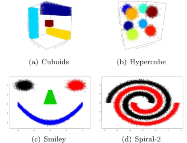
The datasets have been generated using the R package mlbench [24], a collection of standard benchmark problems. The datasets—all composed by 50.000 instances—that have been generated are the following (see Figure 2 for some examples):
• Cassini: 2-dimensional problem with 3 clusters (2 external banana-shaped clusters with a circular cluster between them).
• Cuboids: 3-dimensional problem with 3 cuboids and a small cube in the middle of them.
• Hypercube: 8 spherical Gaussians distributed at the corners of a 8-dimensional cube.
• Shapes: a Gaussian, square, triangle and wave in 2 dimensions.
• Simplex: 4 spherical Gaussians distributed at the corners of a 4-dimensional simplex.
• Smiley: 2 Gaussian eyes, a trapezoid nose and a parabola mouth (with vertical Gaussian noise). • Spirals-1: 2 entangled spirals without noise. • Spirals-2: 2 entangled spirals with noise.
(a) Cuboids (b) Hypercube
(c) Smiley (d) Spiral-2
Figure 2 Illustration of the synthetic datasets used in the experiments.
6 Computational Results
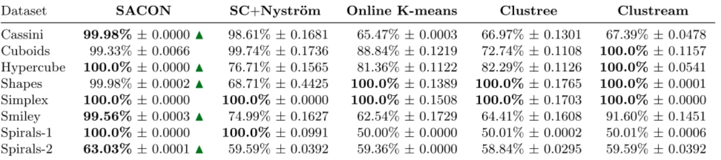
Table 1 presents the results achieved by the algorithms in each dataset. As we can observe, the proposed SACON algorithm obtains very good results overall.
In the case of Cassini dataset, SACON obtains the best results—the statistical test shows that SACON is significantly better than SC+Nystr¨om. It is important to remark that the standard deviation (SD) of SACON is 0, which means that these results are stable. SC+Nystr¨om also obtains good results, while the remaining algorithms obtain poor results. The Cassini dataset has two sections that can be easily defined using a Gaussian distribution, but when the number of instances is high the boundaries between these distributions are harder for the discrimination process; SC+Nystr¨om is also sensitive to the noise produced in this situation.
For Cuboids dataset, Clustream obtains the best median results (100.0%) followed by SC+Nystr¨om (99.74%), with SACON achieving close results (99.33%). SACON is the most stable of the algorithms in this dataset (0.0066 of SD). The Wilcoxon test shows that there is not statistical difference between the SACON and SC+Nystr¨om.
Hypercube results show that SACON is able to discriminate the clusters perfectly. Clustream also obtains good results during the discrimination process. SC+Nystr¨om, Clustree and Online K-means have problems to discriminate the cluster distribution. This dataset is challenging due to the large quantities of data, which introduces noise during the cluster separation (Figure 2(b)). The algorithms are also less stable than SACON (the SD of SACON is 0). Again, SACON is statistically significantly better than SC+Nystr¨om.
In the case of Shapes, the best results according to the median are achieved by Clustream, Clustree and Online K-means. SACON obtains good results (99.98%) and it is also very stable (the SD is 0.0002). SC+Nystr¨om obtains the worst results (68.71%). According to the statistical test, SACON is statistically significantly better than SC+Nystr¨om again.
Table 1 Median and standard deviation accuracy results obtained by each algorithm, measured over 100 executions. Values in bold show the best results. The!symbol indicates the datasets where the results of SACON are statistically significantly better than the results of the benchmark SC+Nystr¨om algorithm.
Dataset SACON SC+Nystr¨om Online K-means Clustree Clustream
Cassini 99.98%±0.0000! 98.61%±0.1681 65.47%±0.0003 66.97%±0.1301 67.39%±0.0478 Cuboids 99.33%±0.0066! 99.74%±0.1736 88.84%±0.1219 72.74%±0.1108 100.0%±0.1157 Hypercube 100.0%±0.0000! 76.71%±0.1565 81.36%±0.1122 82.29%±0.1126 100.0%±0.0541 Shapes 99.98%±0.0002! 68.71%±0.4425 100.0%±0.1389 100.0%±0.1765 100.0%±0.0001 Simplex 100.0%±0.0000! 100.0%±0.0000 100.0%±0.1508 100.0%±0.1703 100.0%±0.0000 Smiley 99.56%±0.0003! 74.99%±0.1627 62.54%±0.1729 64.41%±0.1608 91.60%±0.1451 Spirals-1 100.0%±0.0000! 100.0%±0.0991 50.00%±0.0000 50.01%±0.0002 50.01%±0.0006 Spirals-2 63.03%±0.0001! 59.59%±0.0392 59.36%±0.0000 58.84%±0.0295 59.59%±0.0392
Simplex is easy for all algorithms. The median values show that they obtain the maximum results. These results are a consequence of the data structure —in this case, they only need to discriminate spheres, which is the simplest clustering problem. There is not statistical difference between SACON and SC+Nystr¨om. Smiley results show that SACON obtains the best discrimination results (99.59%). The remaining algorithms have problems generating the clusters. This dataset represents a continuity-based problem, therefore only SC+Nystr¨om, Clustream and SACON can discriminate the boundaries (Figure 2(c)). SACON is statistically significantly better than SC+Nystr¨om.
TheSpiral-1 dataset tests show how the algorithms can deal with continuity datasets without noise. In this case, SACON and SC+Nystr¨om obtain the best results (100.0%); Online K-means, Clustree and Clustream have problems discriminating the spirals, which means that these algorithms are not able to deal with pure continuity-based problems. There is not statistical difference between SACON and SC+Nystr¨om.
The Spiral-2 dataset introduces noise to Spiral-1 (Figure 2(d)). In this case, the results of SACON are worse than in the previous Spiral-1 dataset, as expected, but it obtains the best and more stable results. The results of the remaining algorithms show that there is a good minimal solution and all of them are close to this solution (around the 59%), however, they still find problems discriminating the spirals. SACON is statistically significantly better than SC+Nystr¨om.
6.1 Discussion
SACON shows competitive results identifying manifolds when is applied to continuity-based data—such as Cassini, Shapes, Smiley and Spirals—while the remaining algorithms have problems (e.g., in Spirals, which is a pure continuity-based problem). It also performs better than the rest when we add noise to the dataset. The algorithm also obtains more stable results than the others according to the standard deviation. The spectral transformation in combination with the ACO clustering procedure is probably the main reason for the algorithm performance—the transformation makes the regularities in the data space more apparent and
the ACO global search procedure is able to find the (near-)optimal cluster assignment. The performance is correlated to the type of clustering that this algorithm can face, i.e., continuity-based clustering.
In order to compare the memory usage of the proposed algorithm against SACOC (its predecessor), it is important to remark that SACON uses a matrix of 50,000×500 instances, whereas SACOC uses 50,000×
50,000 instances. The memory usage of the former is around 0.18 GB while the latter consumes around 18.63 GB. The memory consumption of SACON grows linearly, whereas SACOC grows exponentially. The remaining algorithms are not spectral algorithm, with the exception of SC+Nystr¨om—i.e., they do not use a similarity matrix. Regarding the memory consumption, the online algorithms only keep in memory the information about the centroids they are using (similar to K-means), i.e., the memory grows according to the number of centroids.
7 Conclusions
This paper proposed an improvement of the SACOC algorithm [14] using the a Nytr¨om extension [5]. The new algorithm, called SACON, applies the spectral transformations and the Nystr¨om extension to the original search space in order to cluster the data in the projective space. The projection consists on transforming the original data into a graph-based representation (through a similarity graph) and calculate its Laplacian matrix. During this calculation, the Nystr¨om extension guarantees that the Laplacian calculation is accurate enough using less information. Once the Laplacian has been obtained, the eigenvectors are extracted and normalized to generate the projective space—this extraction also applies the Nystr¨om extension in order to reduce the memory usage.
The proposed SACON algorithm shows good results in the studied datasets. It is able to discriminate manifolds and continuity-based clusters with more stable results in dense datasets, when compared to Spectral Clustering using the Nystr¨om extension and modern online clustering algorithms. The future work will be mainly focused on running experiments with real-world
Improving the SACOC algorithm through the Nystr¨om extension for Dense Manifold Data Analysis 9 large datasets, in particular large datasets with cluster
intersections.
Acknowledgement
This work has been supported by the research projects: TIN2014-56494-C4-4-P, CIBERDINE S2013/ICE-3095, SeMaMatch EP/K032623/1 and Airbus Defence & Space (FUAM-076914 and FUAM-076915).
References
[1] C. Chu, S.K. Kim, Y. Lin, Y. Yu, G. Bradski, A.Y. Ng, and K. Olukotun. Map-reduce for machine learning on multicore. Advances in Neural Information Processing Systems, 19:281, 2007. [2] S. Guha, N. Mishra, R. Motwani, and
L. O’Callaghan. Clustering data streams. In
Proc. 41st Annual Symposium on Foundations of Computer Science, pages 359–366. IEEE, 2000. [3] D.T. Larose. Discovering Knowledge in Data. John
Wiley & Sons, 2005.
[4] H.D. Men´endez, D.F. Barrero, and D. Camacho. A genetic graph-based approach for partitional clustering.International Journal of Neural Systems, 24(03), 2014.
[5] C. Fowlkes, S. Belongie, F. Chung, and J. Malik. Spectral grouping using the nystrom method.
IEEE Trans. on Pattern Analysis and Machine Intelligence, 26(2):214–225, 2004.
[6] M. Dorigo and M. Birattari. Ant colony optimization. InEncyclopedia of Machine Learning, pages 36–39. Springer, 2010.
[7] F.E.B. Otero, A.A. Freitas, and C.G. Johnson. Inducing decision trees with an ant colony optimization algorithm. Applied Soft Computing, 12(11):3615–3626, 2012.
[8] H.D. Men´endez, F.E.B. Otero, and D. Camacho. MACOC: a medoid-based ACO clustering algorithm. In Swarm Intelligence, pages 122–133. Springer, 2014.
[9] P. Kranen, I. Assent, C. Baldauf, and T. Seidl. The clustree: indexing micro-clusters for anytime stream mining. Knowledge and Information Systems, 29(2):249–272, 2011.
[10] C.C. Aggarwal, J. Han, J. Wang, and P.S. Yu. A framework for clustering evolving data streams. In
Proc. of the 29th International Conference on Very Large Data Bases - Volume 29, pages 81–92, 2003. [11] U. von Luxburg. A tutorial on spectral clustering.
Statistics and Computing, 17(4):395–416, 2007.
[12] A. Karatzoglou, A. Smola, K. Hornik, and A. Zeileis. kernlab – An S4 Package for Kernel Methods in R. Journal of Statistical Software, 11(9):1–20, 2004.
[13] U. von Luxburg, M. Belkin, and O. Bousquet. Consistency of spectral clustering. The Annals of Statistics, 36(2):555–586, 2008.
[14] H.D. Men´endez, F.E.B. Otero, and D. Camacho. SACOC: A spectral-based ACO clustering algorithm. In Intelligent Distributed Computing VIII, pages 185–194. Springer, 2015.
[15] R.S. Parpinelli, H.S. Lopes, and A.A. Freitas. Data mining with an ant colony optimization algorithm.
IEEE Trans. on Evolutionary Computation, 6(4):321–332, 2002.
[16] F.E.B. Otero, A.A. Freitas, and C.G. Johnson. A New Sequential Covering Strategy for Inducing Classification Rules With Ant Colony Algorithms.
IEEE Trans. on Evolutionary Computation, 17(1):64–76, 2013.
[17] C. Blum and K. Socha. Training feed-forward neural networks with ant colony optimization: An application to pattern classification. InProc. of the 5th International Conference on Hybrid Intelligent Systems, pages 233–238, 2005.
[18] M. Borrotti and I. Poli. Na¨ıve bayes ant colony optimization for experimental design. InSynergies of Soft Computing and Statistics for Intelligent Data Analysis, pages 489–497. Springer, 2013. [19] Y. Kao and K. Cheng. An ACO-Based Clustering
Algorithm. InAnt Colony Optimization and Swarm Intelligence, pages 340–347. Springer, 2006.
[20] L. Ashok and D.W. Messinger. A spectral image clustering algorithm based on ant colony optimization. In Proc. of SPIE (Algorithms and Technologies for Multispectral, Hyperspectral, and Ultraspectral Imagery XVIII), volume 8390, 2012. [21] O.A. Mohamed Jafar and R. Sivakumar. Ant-based
clustering algorithms: A brief survey. International Journal of Computer Theory and Engineering, 2:787–796, 2010.
[22] P.S. Shelokar, V.K. Jayaraman, and B.D. Kulkarni. An ant colony approach for clustering. Analytica Chimica Acta, 509(2):187–195, 2004.
[23] A. Ng, M. Jordan, and Y. Weiss. On Spectral Clustering: Analysis and an algorithm. InAdvances in Neural Information Processing Systems, pages 849–856, 2001.
[24] F. Leisch and E. Dimitriadou. mlbench: Machine Learning Benchmark Problems, 2010. R package version 2.1-1.