Weakly Supervised Learning for Semantic Segmentation

Weakly Supervised Learning for

Semantic Segmentation

Brett D. Whitford

Supervisor:

Dr. James W. Davis

Laboratory For Artificial Intelligence Research

Ohio State University

Presented in Partial Fulfillment of the Requirements for the Degree

B.S. in Electrical and Computer Engineering with Honors Research

Distinction in the College of Engineering at Ohio State University

© Copyright by Brett D. Whitford

Abstract

We propose a novel framework for semantically segmenting images at the pixel-level given a dataset labeled only at the image-level. The intention of this model is to remove the expensive, time consuming, and unreliable process of densely labeling image datasets at the pixel-level. To accomplish this, our algorithm lays a framework to mesh techniques from unsupervised learning with the same deep convolutional neural network architectures that produce state-of-the-art results on fully-supervised datasets. The first pivotal contribution that separates our proposed algorithm from existing methods is that we avoid hallucinating a per pixel ground truth. We achieve this by maintaining a per pixel confidence distribution across classes and leveraging an expectation maximization framework to optimize these distributions using the image-level labels. Secondly, we propose a dataset score metric to measure how a tractable a given dataset is for the weakly supervised setting. We demonstrate that our proposed algorithm allows us to accurately segment high entropy problems typically intractable for weak supervision.

Acknowledgments

My research was very much a team effort from the entire Computer Vision Laboratory and I sincerely thank everyone who made a contribution. However, special acknowledgment is due to Professor James Davis for his continuous support, guidance, and encouragement throughout this journey.

I also would like to extend acknowledgments to Professor Rephael Wenger, Christopher (Chris) Menart, and Muhammad (Mo) Akbar. I am very thankful for Professor Wenger’s willingness to sit on my defense committee and for his valuable feedback on this thesis. Additionally, without Chris and Mo’s intimate knowledge of implementing DCNNs, this work would not have been possible.

Chris’ talent for implementing and, more importantly, debugging both MAT-LAB code and TensorFlow code was invaluable. Mo’s experience was instrumental in the implementation of the weakly supervised framework on top of the RefineNet code base.

Finally, additional thanks is due to both the Ohio Supercomputer Center [2] for providing access to computational resources that allowed this thesis to be possible and to the Ohio State College of Engineering for providing funding for the research.

Vita

August 1995 . . . Born - Cincinnati, OH, USA

May 2018 . . . B.S. Electrical and Computer Engineering, OSU

Fields of Study

Major Field: Department Of Electrical and Computer Engineering Program of Study: Computer Engineering

Table of contents

List of figures viii

1 Introduction 1

1.1 Contributions and Significance . . . 4

1.2 Terminology . . . 5

1.3 Organization . . . 7

2 Related Work 8 2.1 Review of Network Architectures . . . 8

2.1.1 Fundamental Architectures . . . 9

2.1.2 Fully Supervised Semantic Segmentation . . . 11

2.1.3 Weakly Supervised Semantic Segmentation . . . 12

2.2 Takeaways . . . 14

3 Design Methodology 15 3.1 Preliminary Investigation . . . 15

3.2 Parameter Gathering . . . 17

3.3 Simulation, Prototyping, and Testing . . . 18

3.4 Documentation . . . 19

4 Framework Overview 21 4.1 Background . . . 21

4.1.1 Expectation Maximization . . . 21

4.1.2 Binary Dissimilarity . . . 22

4.2 Proposed Framework . . . 24

4.2.1 Expectation Maximization Framework . . . 24

4.2.2 Proposed Score Metric . . . 26

5 Results and Analysis 29 5.1 Perceptron Tests . . . 30

5.1.1 Perceptron Test Feature Space . . . 31

5.1.2 Feature Space Generality . . . 32

5.1.3 Interclass Correlation . . . 34

5.1.4 Image Complexity and Dataset Size . . . 35

5.2 Stochastic Gradient Descent Failure Modes With A CNN . . . 36

6 Conclusion 38 6.1 Summary . . . 38

6.2 Contributions and Significance . . . 39

6.3 Future Work . . . 40

List of figures

1.1 The left images shows the task of image classification. On the right is an example of how semantic image segmentation partitions an image into different parts and object classes. [10] . . . 1 1.2 Transfer learning within the domain of language identification from

[12]. . . 3 1.3 On the left is a picture from the PASCAL VOC 2012 dataset [9]

with an associated image-level-label. On the right is the associated pixel-wise labeling that was done by hand. Our proposed model would only need image-level labels to train a model to segment an image at the pixel-level. . . 5 2.1 A iterative outline of the perceptron algorithm [20] . . . 9 2.2 An illustration of the architecture of AlexNet [15] . . . 10 2.3 The fundamental building block of residual learning proposed in the

ResNet framework [11]. . . 10 2.4 Architecture pipeline for the RefineNet model [16]. . . 11 2.5 Architecture pipeline for the DeepLab model [4]. . . 12 2.6 End-to-end pipeline of the Papandreou et al.’s model under the

setting where only image-level labels are present. Note that the Deep Convolution Neural Network used is the DeepLab model [22]. 13 2.7 Multiple instance learning framework of [27]. . . 14

4.1 K-means psuedocode showing an iterative implementation of “hard” expectation maximization from [20]. . . 22 4.2 (a) Initial (random) values of the parameters. (b) Posterior

respon-sibility of each point computed in the first E step. The degree of redness indicates the degree to which the point belongs to the red cluster, and similarly for blue; this purple points have a roughly uniform posterior over clusters. (c) We show the updated parameters after the first M step. (d) After 3 iterations. (e) After 5 iterations. (f) After 16 iterations. Figure and caption from [20]. . . 23 4.3 Generalizable algorithm for our proposed weakly supervised

frame-work. Batch construction metrics are further explained in Section 4.2.2. . . 25 4.4 The end-to-end pipeline of our proposed expectation maximization

framework. Portions in blue represent the exception step while areas in red represent the maximization step. . . 25 4.5 Two-dimensional demonstration of IoU. [24]. . . 27 5.1 Example of a pseudo-image. For each image, there is one associated

image-level label that contains a binarized list of classes within the image’s pixels. The pixels themselves are ten two-dimensional points, consisting of two features (R,G). Each pixel has an associated ground truth class (the third feature in the tuple) which is used for evaluation but is unavailable during training. . . 30 5.2 Initialization of two-dimension feature space. Each cluster represents

one of 9 linearly separable classes. . . 32 5.3 On the right is a sample segmentation of the two-dimensional feature

space. On this left, we see an image with ten associated pixels. Pixels from this image are plotted as stars in the feature space. . . 33

5.4 Evolution of the feature space over 11 iterations of the expectation maximization algorithm. The number to the left of each feature space division is the current iteration of expectation maximization. 33 5.5 Correlation vs. Dissimilarity. . . 35 5.6 Accuracy vs. the number of one-hots. . . 36 5.7 Failure of RefineNet to segment a basic image contain blocks of color. 37

Chapter 1

Introduction

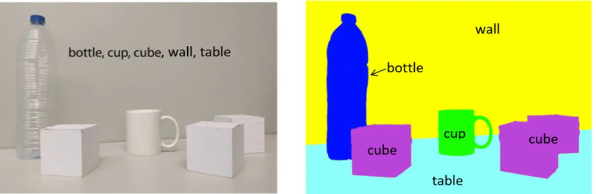
Semantic image segmentation is the task of simultaneous object recognition and segmentation. For every pixel within a given image, the segmentation model must predict a label that corresponds to a semantic object classes such as bottle, cup, cube, wall, or table as seen in the right side of Figure 1.1. This is a fundamen-tal problem in computer vision and has received significant attention in recent years.

Fig. 1.1 The left images shows the task of image classification. On the right is an example of how semantic image segmentation partitions an image into different parts and object classes. [10]

The task of semantic segmentation is significantly more challenging than classification, which is shown on the left of Figure 1.1. Classification can be thought of as the most coarse task in computer vision—for a given input there is

only one prediction of the constituent elements. In contrast, the goal of semantic segmentation is a much more refined output since for every single pixel-wise location a dense prediction across classes must be made.

This refined incorporation of semantic information is what makes the challenge of segmentation so desirable in many of today’s applications, such as autonomous driving [8], image search engines [6], or video surveillance [26]. For tasks such as video surveillance, it does not suffice to only know what is in an image—one must also understand the elements in context in order to make informed decisions. A person standing next to the window of a house has a much different contextual meaning than a pedestrian on the sidewalk in the domain of video surveillance. To determine this context, a semantic segmentation model must have an understanding of the localization of all instances of each class within an image.

Recently, Deep Convolutional Neural Networks have emerged as the state-of-the-art for semantic segmentation [1, 3, 4, 16, 22, 23]. These models are able to incorporate both spacial and semantic information through the use of convolutional layers. Non-linearities introduced through the activation functions of the network’s individual neurons enable the model to encode complex mapping functions.

The ability for deep neural networks to learn sufficiently general features has proven to be a major strength of deep architectures. It is common to reuse features instead of random initialization to allow for transfer learning [21]. This is highly desirable in many settings due to the fact 0it is often not possible to train a deep neural network from scratch due to limitations in available training data. Instead, the lower levels of an existing network are kept (theoretically containing the more general features from the previous training) while the end of the old network is cut off and retained to learning specific feature from the new domain, as show in Figure 1.2.

Methods for artificially boosting available training data exist, such as data augmentation. By applying transformations such as flipping, cropping, rotation,

Fig. 1.2 Transfer learning within the domain of language identification from [12].

or scaling, new samples are able to be synthetically produced. This increases the size of the dataset and increases model performance [28].

However, neither transfer learning nor data augmentation are not substitutes for collecting a proper dataset. Deep convolutional neural network architectures often require large and diverse datasets of images densely labeled at the pixel-level for training under full supervision. Creating such a dataset is a expensive, time-consuming, and unreliable process.

This has caused the research domain of computer vision to converge around a select few fully-annotated datasets that have been released publicly, such as PASCAL Visual Object Challenge [9], PASCAL Context [19], Microsoft Common Objects in Context [17], CityScapes [5], and SiftFlow [18]. These datasets are taken to be representative enough for training in a variety of semantic segmentation problems.

Clearly, a key constraint on state-of-the-art architectures is the reliance on pixel-wise annotated images for training. In this thesis we address this issue by proposing a novel framework for semantically segmenting images at the pixel-level given a dataset labeled only at the image-level. This method of labeling is know as weak supervision and consists only of a single vector for each image.

1.1

Contributions and Significance

To accomplish segmentation under the weakly supervised setting, our algorithm lays a framework to mesh the expectation maximization (EM) technique from unsupervised learning with the same deep convolutional neural network (DCNN) architectures that produce state-of-the-art results on fully-supervised datasets. Specifically, we present the following pivotal contributions:

Novel EM Algorithm- Our proposed algorithm is fundamentally different from existing methods since we avoid hallucinating a per pixel ground truth. We achieve this by maintaining a per-pixel confidence distribution across classes and leveraging an expectation maximization framework to optimize these distributions using the image-level labels. Additionally, our proposed algorithm takes the atypical perspective of masking what we know is not in the image instead of boosting what we knowis in the image.

Dataset Score Metric - We propose a dataset score metric to measure how a tractable a given dataset is for the weakly supervised setting. We demonstrate that our proposed algorithm allows us to accurately segment high entropy problems typically intractable for weak supervision.

In Figure 1.3, the advantage of our proposed method is made clear. The expensive, time consuming, and unreliable process of densely labeling image datasets at the pixel-level has been removed. Our proposed segmentation system

abstracts the labeling task to a simple binary decision—whether or not a particular class is in the image.

Fig. 1.3 On the left is a picture from the PASCAL VOC 2012 dataset [9] with an associated image-level-label. On the right is the associated pixel-wise labeling that was done by hand. Our proposed model would only need image-level labels to train a model to segment an image at the pixel-level.

We achieve this by maintaining a per pixel confidence distribution across classes and leveraging an expectation maximization framework to optimize these distributions using the image-level labels. We theoretically prove that this allows use to accurately segment high entropy problems typically intractable for weak supervision.

1.2

Terminology

Throughout this thesis, we will refer to deep neural network architectures, the image training set, and model parameters in different manners specific to the domain of computer vision and weak supervision. The following are the naming conventions.

Fully Supervised Learning - The task of learning a function that maps a input pixel to an output pixel based upon input-output pairs. In context of this thesis, full supervision implies every pixel of the training images is mapped to an explicit class label.

Weakly Supervised Learning- The task of learning a function that maps a input pixel to an output pixel based upon coarse input-output pairs. In context of this thesis, weak supervision refers to the scenario where the training images consist of a binary image-level label mapped to individual pixels.

Semi-Supervised Learning - The task of learning a function that maps a input pixel to an output pixel based upon a mixture of labeled and unlabeled output pairs. Typically, there are a small amount of labeled images or image sections combined with a large amount of unlabeled images.

Unsupervised Learning - The task of learning a function that describes the underlying structure of input image without any labeled outputs. This is an undesirable formulation for semantic segmentation, since unsupervised methods cannot learn class mappings—the fundamental tenant of semantic segmentation.

Deep Learning vs. Convolutional Neural Networks - Strictly speak-ing, deep convolutional neural networks are a subset of deep learning. All deep learning does not use convolutional layers and all convolutional neural networks are not deep. However, in the context of this thesis, the terms “deep learning”, “deep learning architecture”, and “convolutional neural network” refer to algorithms that model high-level abstractions in images by using a deep graph with multiple convolutional layers.

Information Entropy - The average amount of information present in a dataset. In the context of this thesis, entropy will refer to the quantity representing the average amount of information in a binarized image-level label or the set of all image-level labels in a dataset. High entropy training

datasets are very desirable for weak supervision while low entropy datasets are quite challenging.

One-hot Vector - A one dimensional vector that contains one non-zero element. This represents the maximally informative labeling. Weakly super-vised learning converges to fully supersuper-vised learning in the scenario where all image-level labels are one-hot vectors.

N-hot Vector- A one dimensional vector that contains N non-zero elements. In this thesis, an N-hot vector refers to a binarized image-level label containing N non-zero elements. Weakly supervised learning converges to unsupervised learning in the scenario where all image-level labels are N-hot vectors where N is the length of the non-singleton dimension.

Full Rank Matrix- A matrix of which the rank is equal to the total number of unique classes present in the training dataset.

1.3

Organization

This thesis is organized into six main parts. Chapter 1 has outlined the challenge of semantic segmentation and introduces the significance of this thesis. Chapter 2 begins with a review of current work relevant to semantic segmentation and evaluates the state of weakly supervised methods. Chapter 3 describes the holistic research methodology used to design this thesis. Chapter 4 provides an overview of the proposed framework and how it was implemented. Chapter 5 lays out the results from the experiments conducted in our work. Finally, Chapter 6 concludes the thesis with an overview of the proposed methods and future work to be completed.

Chapter 2

Related Work

In recent years, there has been an explosion of research in computer vision. Advancements in deep learning architectures and increases in computational power have driven the state-of-the-art research in semantic image segmentation. In this section, we will examine the current fully supervised and weakly supervised neural network models that provide the theoretical basis for our proposed framework.

2.1

Review of Network Architectures

There is significant overlap between the architectures that perform highly under full supervision and weak supervision. Therefore it is necessary to understand the current state of research being conducted in the fully supervised setting and subsequently how it is built upon to handle weakly supervised setting. Furthermore, one must be familiar with the fundamental architectures that form the basis for our model.

2.1.1

Fundamental Architectures

Several fundamental architectures were used in our work, both explicitly and implicitly as building blocks for more advanced fully supervised architectures. The basics of these frameworks are outlined here.

Perceptron Proposed by Rosenblatt in 1958, the perceptron was one of the first neural networks ever produced [25]. The perceptron is an algorithm for learning a linear binary classifier and can be though of as representing a single layer neural network as shown in Figure 2.1.

Fig. 2.1 A iterative outline of the perceptron algorithm [20]

The perceptron convergence theorem states that for any data set which is linearly separable the perceptron learning rule is guaranteed to find a solution in a finite number of steps. This is to say that the perceptron algorithm will converge to a feature vector that is able to classify all training examples provided that they are linearly separable. Therefore, the perceptron can represent the boolean functions AND, OR, NAND, and NOT, but not XOR.

AlexNet AlexNet famously emerged as the pioneering deep convolutional neural network in 2012, winning the ImageNet Large Scale Visual Recognition Challenge with a a top-5 error of 15.3 [15]. The architecture consisted of of 5

convolutional layers, max-pooling layers, dropout layers, and 3 fully connected layers as show in Figure 2.2. This work started was responsible for the explosion of interest in convolutional neural networks.

Fig. 2.2 An illustration of the architecture of AlexNet [15]

ResNet ResNet is a pioneering residual learning framework that opened the door for training networks that are much deeper than the previously used architectures. The layers are designed as residual functions with reference to the layer inputs, as show in Figure 2.3. He et. al provide comprehensive empirical evidence showing that these residual networks are easier to optimize, and can gain accuracy from considerably increased depth [11].

Fig. 2.3 The fundamental building block of residual learning proposed in the ResNet framework [11].

2.1.2

Fully Supervised Semantic Segmentation

Several fully supervised architectures were used in our work as modules for our weakly supervised formulation. The basics of these frameworks are outlined here.

RefineNet Released in 2016 by Lin et. al [16], RefineNet achieved a state-of-the-art intersection-over-union score of 83.4 on the challenging PASCAL VOC 2012 dataset. The authors proposed a novel multi-path refinement network that aims to exploit features at multiple levels to achieve pixel-wise semantic segmenta-tion. RefineNet refines low-resolution semantic features with fine-grained low-level features in a recursive manner to generate high-resolution semantic feature maps.

Fig. 2.4 Architecture pipeline for the RefineNet model [16].

DeepLab The DeepLab model [4] employs atrous convolution as a powerful tool to control the resolution of feature responses computed by networks, as well as to adjust each convolution filter’s field of view. The authors employ atrous convolution in parallel in order to capture capture multi-scale context by adopting multiple atrous rates.

Furthermore, the authors augment the previously proposed Atrous Spatial Pyramid Pooling module from a previous version of DeepLab, which probes convolutional features at multiple scales, with image-level features encoding global context and further boost performance.

Fig. 2.5 Architecture pipeline for the DeepLab model [4].

The proposed “DeepLabv3” system attains comparable performance with other state-of-art models on the PASCAL VOC 2012 semantic image segmentation benchmark.

2.1.3

Weakly Supervised Semantic Segmentation

A recent work by Papandreou et al. formed the basis of our weakly supervised formulation. Additionally, we inspect the basics of the work of Vezhnevets et al. who approach our same formulation of weak supervision from a fundamentally different perspective.

Papandreou et al. Papandreou et al. [22] develop expectation maximiza-tion methods for semantic image segmentamaximiza-tion model training under a variety of weakly supervised and semi-supervised settings. Of particular importance to

this thesis, is their proposed algorithm for the setting where dataset labels are restricted to the image-level label.

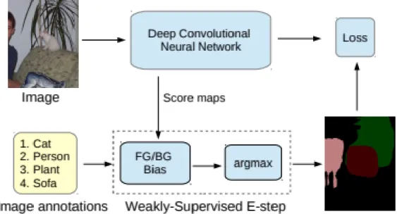
Fig. 2.6 End-to-end pipeline of the Papandreou et al.’s model under the setting where only image-level labels are present. Note that the Deep Convolution Neural Network used is the DeepLab model [22].

As seen in Figure 2.6, the authors take the approach of using foreground/background boosting in order to drive their expectation maximization framework toward the optimal solution. Additionally, it is important to recognize this architecture adopts hard expectation maximization, as they take the argmax of the biased score map for use as the target in the maximization step.

Vezhnevets et al. Vezhnevets et al. [27] approach weakly supervised semantic segmentation from the perspective of multiple instance learning. They use a Semantic Texton Forest as the basic framework and extend it for the multiple instance learning setting. An external task of geometric context estimation is also used to improve on the task of semantic segmentation.

This setting is concerned with a learning scenario where samples come in multisets (bags) and labels are known only for these bags, but not for the instances themselves.

Fig. 2.7 Multiple instance learning framework of [27].

2.2

Takeaways

The main branch of development in the domain of computer vision is driven by fully supervised models. State-of-the-art frameworks are often built as intelligent modifications of a select few architectures that have been proposed in recent years, such as AlexNet or ResNet. These models produce high accuracy on in domain datasets and are able to successfully generalize to out of domain problems through the use of transfer learning.

Development in settings other than full supervision does not require the redesign of these prominent networks. Rather, as we have seen with Papandreou et al., models that provide excellent results in fully supervised scenarios can be successfully employed in the weakly supervised scenario when placed inside of a structure that leverages image-level labels. Although weakly supervised model are not as robust to dataset limitations, there is promising work showing that they can adapt fully supervised models to learn in settings with little information available.

Chapter 3

Design Methodology

In this chapter, we provide an high-level overview of the design process for our proposed weakly supervised semantic segmentation algorithm. The work in this thesis follows a rigorous design process that included preliminary investigation, parameter gathering, simulation and prototyping, testing, and documentation. Table 3.1 below gives an outline of the project.

Table 3.1 Design Timeline

Autumn 2016• Literature review

Spring 2017• Preliminary investigation, documentation Autumn 2017• Simulation, prototyping, documentation

Spring 2018• Testing, research forum presentation, thesis defense

3.1

Preliminary Investigation

Preliminary investigation began with a semester-long research review. At this point in time, the state-of-the art work in computer vision was reviewed and

investigated. Research from leading conferences in the field of computer vision, such as CVPR, ICCV, ECCV, and BMVC was analyzed. In particular, we looked for areas where there was promising work in the fully supervised scenario that might have potential for modification in a weakly-supervised scenario.

After this semester of research, we identified the fundamental problem that many of the leading frameworks in semantic image segmentation relied heavily on full supervision. The limitations of full supervision, such as the time-consuming labeling process, are very apparent. Pushmeet et al. [14] report that it takes between 15 and 20 minutes to fully annotate an image in this manner—certainly not a reasonable task for the average researcher when datasets that can be up to 200,000 images.

But more importantly, the restriction to image-level labels represented a natural—in a biological context—progression for semantic segmentation to move away from full supervision. Geoff Hinton, a professor of machine learning at the University of Toronto, has said:

When we’re learning to see, nobody’s telling us what the right answers are—we just look. Every so often, your mother says “that’s a dog”, but that’s very little information. You’d be lucky if you got a few bits of information—even one bit per second—that way. [20]

From a biological perspective, it is unnatural to learn under fully supervision. Assuming a pixel-wise labeled 300 x 500 image with 60 possible classes, each training example would have 9000000 bits (1.125 megabytes) of information. Professor Hinton shows this supervision is seven orders of magnitude more that what humans use to learn from visual stimulus.

Suppose instead the same image was only labeled with a binarized image-level label—there would only be 60 bits (7.5 bytes) of information in the label. This is much closer to the biological construction of learning from visual data. We must

learn from the underlying structure of the input data, not dense labels, in order to learn in a more life-like manner. Additionally, we conservatively estimate that labeling an picture at the image-level takes 15 seconds—approximately 60 times faster than pixel-wise labeling.

It was with these considerations in mind that we began to brainstorm a model that could segment an image at the pixel-level only with access to labels at the images-level.

3.2

Parameter Gathering

We then began to layout the requirements for a system that might be able to recreate the performance of a fully supervised model, but only with access to image-level label data. After consideration, we arrived at the following specifications for our model:

Strict Image-level Labeling - The model would strictly have access to image-level labeling. It is sometimes common to have access to a small amount of fully annotated data in some settings of semi-supervision, however, we would not allow for any fully annotated training examples. This would allow us to focus solely on the information gain of the coarsely annotated data.

Architecture Independence - Our weakly supervised formulation would need to be independent of the underlying prediction framework. This is a powerful aspect since we would be able to abstract all low-level implementa-tion details of the underlying framework. We can change out the underlying framework at will in order to have certain convergence conditions or per-formance. Additionally, this allows for our model to hold as segmentation architectures continue to improve.

Specialized Loss Function - We would need a function that maps an prediction onto a real number intuitively representing the “cost” associated with the error of the prediction. This function would have to quantity loss under the constraints of image-level labels.

Data Entropy Metric - With the access to data being extremely limited in the weakly supervised formulation, we recognized that we would need a metric to determine whether nor not a dataset would be feasible to segment with our framework.

Model Time Complexity- The model would have to be able to achieve its segmentation results in a reasonable amount of time, in especially in the case where the model is not preinitialized. The fully supervised DeepLab model [4] is able to be trained in 3.65 days so we judged that approximately double that is fair for a weakly supervised model.

Model Space Complexity - The model would have to only use an amount feasible for the average research center. Movement toward weak supervision would come at the price of space since we could not afford to throw away any of the information about we know (or information about what we don’t know).

3.3

Simulation, Prototyping, and Testing

The proposed model would have to be simulated on a variety of computers with a variety of architectures and datasets to ensure the specification of the parameters specified in the above section were met. We then conducted simulations and tests on our model prototype in the following scenarios:

High Entropy Data - The first task is to test the weakly supervised architecture on the optimal scenario of high entropy data. High entropy

datasets provided clearer distinctions between classes which improve the model’s ability to correct mistakes. This would be a preliminary test to see if the weakly supervised model was feasible.

Low Entropy Data- A challenging task for weak supervision is low-entropy data. With little information in the label set, distinction between classes are difficult to determine and the model might not be able to be driven toward the optimal solution.

Simple Models- The advantage of training with a simple underlying model is that all theoretical assumptions about convergence are very transparent. This allows for convergence extrapolations from the fully supervised case to carry over to the weakly supervised case.

Advanced Models - While training with a more advanced or complex model might not have simple convergence conditions, it offers more power to train on low entropy datasets. Testing with state-of-the-art models, such as DeepLab, allows us to test what weakly supervised methods are capable of and will be included in future work.

3.4

Documentation

Finally, careful documentation was critical throughout the design process. Many different machines, running a variety of operating system flavors, were used to test and develop our framework on top of a multitude of architectures. The following tools were critical to the centralization and upkeep of documentation.

GitHub - Careful version control of the codebase was maintained through GitHub. This made it simple to move code from computers physically in the lab to the computers and GPUs at the Ohio Supercomputer Center.

BuckeyeBox - BuckeyeBox served as the cloud storage solution for sharing results of the simulations. The advantages of weak supervision come at the price of space complexity so it was integral to have a central storage location for files.

OneNote - OneNote was used as the collaboration platform for taking organized notes. This platform proved to be extremely useful during the literature review, as it allowed for highly systematic storage of marked-up research papers that had been reviewed.

Chapter 4

Framework Overview

Now that the design methodology has been reviewed, we will examine the proposed weakly supervised semantic segmentation framework. The chapter will begin with background on expectation maximization and binary dissimilarity metrics, then go into details in how they were implemented in our model.

4.1

Background

We now begin with the necessary background knowledge to understand the methods we use to implement the weakly supervised framework. Both expectation maximization and binary dissimilarity are introduced here.

4.1.1

Expectation Maximization

Introduced by Dempster et al. in 1977 [7], expectation maximization is a broadly applicable algorithm for computing maximum likelihood estimates from incomplete data. It is a simple iterative algorithm with a closed-form update at each step.

Expectation maximization exploits the fact that if the data were fully observed, then the maximum likelihood estimate should be easy to compute. Each iteration

of the algorithm consists of an expectation step followed by a maximization step. The expectation step of the algorithm infers the missing values, ˆy , given the current set of parameters θ′. The maximization step follows by optimizing the the current parameters with respect to the inferred values. Figure 4.2 shows an illustration of expectation maximization applied to a Gaussian mixture model.

An important divergence in variants of the expectation maximization algo-rithms is when is the expectation step is “hard” or “soft”. An illustration of hard expectation can be see in Figure 4.1 which shows pseudocode for the K-means algo-rithm. The hard assignment of each datapoint to a cluster/class in the expectation step make the formulation “hard”—if you avoid explicit assignment and instead adopt a probabilistic distribution the expectation is considered to be “soft”.

Fig. 4.1 K-means psuedocode showing an iterative implementation of “hard” ex-pectation maximization from [20].

4.1.2

Binary Dissimilarity

The binary feature vector is one of the most common representations of patterns and is the method we use to represent the image-level labels in our weakly supervised formulation. Specifically, binary dissimilarity metrics can be used to quantity the amount of data available in a coarsely-labeled dataset.

Fig. 4.2 (a) Initial (random) values of the parameters. (b) Posterior responsibility of each point computed in the first E step. The degree of redness indicates the degree to which the point belongs to the red cluster, and similarly for blue; this purple points have a roughly uniform posterior over clusters. (c) We show the updated parameters after the first M step. (d) After 3 iterations. (e) After 5 iterations. (f) After 16 iterations. Figure and caption from [20].

The more dissimilar two image-level labels are, the more information is gained since the ultimate goal of semantic segmentation is to learn a function that differentiates between classes.

4.2

Proposed Framework

We will now fully examine the proposed weakly supervised semantic segmen-tation framework. We enumerate the model’s algoritmic heuristics, end-to-end pipeline, and data score metric.

4.2.1

Expectation Maximization Framework

Our proposed expectation maximization algorithm is shown in Figure 4.3. At each iteration, we avoid hallucinating a per-pixel one-hot ground truth by maintaining a probabilistic confidence distribution across classes at every pixel location. This is an important divergence from current state-of-the-art expectation maximization framework since we are adapting a “soft” expectation step rather than a “hard” expectation step.

We additionally adopt a method of leveraging the coarse labeling that is different than the state of the art methods. Instead of boosting classes that are in the image-level label with biases, we mask the distributions that are not in the image-level label for use in the maximization step as seen in line 3 of Figure 4.3.

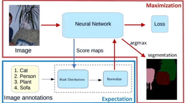
The end-to-end pipeline of our model is show in Figure 4.4. As seen in the diagram, the score maps (the output from the expectation step in the blue region) are passed backed into the prediction architecture (in this case, a deep convolutional neural network) to serve as the network targets in the maximization step (shown in the red region).

Fig. 4.3 Generalizable algorithm for our proposed weakly supervised framework. Batch construction metrics are further explained in Section 4.2.2.

Fig. 4.4 The end-to-end pipeline of our proposed expectation maximization frame-work. Portions in blue represent the exception step while areas in red represent the maximization step.

The final segmentation of an image is obtained by taking the argmax of the score maps across all classes. The goal of our implementation is that the score maps will iteratively converge to the true underlying segmentation, which will allow for increasing information gain through stochastic gradient descent in the maximization step shown in line 6 of Figure 4.3.

4.2.2

Proposed Score Metric

We additionally propose the use of a binary dissimilarity score metric that allows us to evaluate the feasibility of applying weakly supervised methods to an arbitrary image dataset and to intelligently conduct mini-batch stochastic gradient descent.

The metric we use is the Jaccard-Needham dissimilarity index originally proposed by Dr. Paul Jaccard, a professor of botany, in 1901 [13]. Equation 4.1 show the calculation for the dissimilarity index. L11 represents the total number of

classes where the two binarized image-level labels have a value of 1. L10 represents

the total number of classes where the first binarized image-level label has a value of 1 and the second has a value of zero. L01 represents the total number of classes

where the first binarized image-level label has a value of 0 and the second has a value of 1. L00 represents the total number of classes where the two binarized

image-level labels have a value of 0.

dJ =

L10+L01 L10+L01+L11

(4.1) The dissimilarity metric is calculation the is bound 0≤dJ ≤1. Additionally,

the Jaccard-Needham dissimilarity metric can be calculated as the complement of the the Jaccard similarity coefficent sJ, which as see in Equation 4.2 and Equation

sJ =

L11 L10+L01+L11

(4.2)

1−sJ =dJ (4.3)

Intuitively, sJ can be though of as the Intersection over Union (IoU) of two

labels, A and B. This is show in Equation 4.4 and the corresponding complement for dissimilarity is show in Equation 4.5.

sJ = |A∩B|

|A∪B| (4.4)

dJ =

|A∪B| − |A∩B|

|A∪B| (4.5)

When extended to two dimensions, the Jaccard similarity holds a geometric interpretation of high importance for computer vision algorithms. As Figure 4.5 shows, the IoU metric is an excellent proxy for evaluating the localization of a class in an image. For fully supervised strategies, this collapses to a pixel-level Mean Intersection over Union (MIoU) score where the pixel-wise IoU is computed on a per-class basis and then averaged as shown in Equation 4.6.

M IoU = 1 k+ 1 k X i=0 pii k P j=0 pij + k P j=0 pji−pii (4.6)

In this manner our proposed score metric creates a beautiful corollary between the one-dimensional dissimilarity of the input label dataset and the two dimensional output evaluation. The higher the dissimilarity of the input, the higher the similarity of the output to the ground truth. This conclusion is rigorously tested by experiment in Chapter 5.

Chapter 5

Results and Analysis

With a complete understanding of the framework and its underlying algorithms, we now explore experimental results in a variety of scenarios. We begin by applying a multi-layer perceptron to a simplified problem to show the results that form the theoretical basis for our framework to be applied to more advanced architectures (images with a CNN).

We do this by applying our proposed score metric to an array of artificially created two-dimensional datasets to determine which are feasible for our proposed weakly supervised framework. The artificial datasets consist of small images with two values at each pixel (which can be thought of as red and green channels—the blue channel has been removed). A perceptron is then trained to classify the color of each pixel provided only the two values at that pixel. One should note that a perceptron does not leverage any spatial information when making predictions (there are no convolutional layers) and therefore could not be used for segmentation outside of this specific artificial formulation. However, the transparent convergence conditions of the perceptron allow us to carefully delineate which datasets are tractable for weakly supervision and which ones are not.

Following these tests, we show application of our score metric to batch con-struction failure modes in a CNN during mini-batch stochastic gradient descent.

This work is used to motivate the approach and in future work we use the results shown in this section to apply our framework to images with a CNN.

5.1

Perceptron Tests

The perceptron framework is used to understand our model under a variety of artificially created scenarios in this section. Before enumerating these tests, one must understand the motivation for diverging from the three-channel image segmentation to two-channel “pseudo-image” segmentation.

Fig. 5.1 Example of a pseudo-image. For each image, there is one associated image-level label that contains a binarized list of classes within the image’s pixels. The pixels themselves are ten two-dimensional points, consisting of two features (R,G). Each pixel has an associated ground truth class (the third feature in the

tuple) which is used for evaluation but is unavailable during training.

In these tests, we create an analogous setting to the image segmentation problem—the data is labeled at a level of abstraction above model predictions.

However, we project the segmentation problem from three dimensions (R, G, B) on to a two dimensional space (R, G). An example of an image in this space is given in 5.1. The motivation of testing within this space is ease of visual understanding. In two dimensions, we can watch the models’ segmentation of the entire feature space—all pseudo-pixels from every pseudo-image—be classified at each iteration of the algorithm. Essentially, this scenario allows us to holistically view a models’ generality across every class, at any given time, without concentrating on a particular training example or object class.

The idea is that we eliminate the complicated black box of convolutional neural networks predictions. We concentrate in this chapter on why classification changes with respect to the input features and the simplicity of the two-dimensional perceptron makes this straightforward. It is intuitive to use these tests to lay the framework for the construction of algorithms to improve the weakly supervised performance of CNNs that do not hold as explicit of convergence conditions.

5.1.1

Perceptron Test Feature Space

We begin by constructing an artificial two-dimensional dataset that represents a feature space of nine linearly separable two-dimensional Gaussian distributions. This allows for transparency in the convergence conditions—if the model is not able to fully segment the feature space we can infer the dataset is intractable.

Figure 5.2 shows a sample initialization of the feature space. Each point in the feature space represents an individual instance of a class (at a pixel in an image). Note that it is possible for more then one instance of a class to be in an image if it is in the image-level label (i.e. at multiple pixels) and also that if a class is in the image-level label it is guaranteed to be present in the image.

The right portion of Figure 5.3 shows a sample segmentation of the feature space after convergence of the expectation maximization algorithm. Each of the

Fig. 5.2 Initialization of two-dimension feature space. Each cluster represents one of 9 linearly separable classes.

nine colors painted in the background represent the most probable class at that point in the feature space with the current model parameters. Note that the model parameters will be updated at every maximization step of the algorithm and there the divisions of the feature space will shift. Points classified correctly are plotted as black dots, will incorrectly classified points are plotted as red X’s.

5.1.2

Feature Space Generality

The first experiment we conduct is to observe the generality of the model’s classification of the entire two-dimensional feature space as it evolves over time. The number of classes per pseudo-image, R, is set to be 3. The total number of images containing every class in its label,H, is set to be 100. The total number of two-dimensional Gaussian distributions,K, producing unique classes is set to be 9.

Fig. 5.3 On the right is a sample segmentation of the two-dimensional feature space. On this left, we see an image with ten associated pixels. Pixels from this image are plotted as stars in the feature space.

Fig. 5.4 Evolution of the feature space over 11 iterations of the expectation maximization algorithm. The number to the left of each feature space division is the current iteration of expectation maximization.

Over time, we see the model learn to differentiate between all 9 classes. Note how in iteration 1 and 2 neither the gray class nor the blue class are in the feature space classification. Only in iteration 5 are all classes present within the plotted bound of the feature space. By iteration 11, the model has fully converged with over 99% accuracy.

5.1.3

Interclass Correlation

A simple way to substantially decrease the average dissimilarity score of the entire dataset is to force a correlation between a grouping of classes. In order to test the model’s ability to perform under a range of dissimilarity scores, we conduct an array of experiments that vary the correlation of Class 1 with Class 2 (each an arbitrary Gaussian cluster in the feature space show in Figure 5.2).

We see that the higher the dissimilarity score, the faster the model is able to converge. In this test, an iteration is full forward pass across the whole dataset in the expectation step. Therefore, we are able to conclude that higher dissimilarity score tend to mean weak supervision is more feasible.

In this test, convergence was set to be greater than or equal to 97% validation accuracy. If the expectation maximization model is not able to converge in 1000 iterations, we conclude that the model is stuff in a local optima and will not be able to escape and thus has failed.

The first failure occurs at a dissimilarity score of approximately 0.33, however, there are examples of the model succeeding to segment an image with a dissimilarity score as low as 0.15. We conclude that while the dissimilarity score give a good generalization of whether the model is tractable with the given dataset, it is also important to take a close eye to all interclass correlations that might not be fully reflected in the score metric. A high interclass correlation can render a

dataset intractable even if relatively good data diversity can produce a mediocre dissimilarity score.

Fig. 5.5 Correlation vs. Dissimilarity.

5.1.4

Image Complexity and Dataset Size

Next, we look to understand how the complexity of an image affects the ability of our weakly supervised framework to generalize. In order to test this, we start with just one full-rank copy of a label in the form of N-hots. We then increase the number of copies of the N-hot matrix available during training.

Figure 5.6 shows the results from the experiment. Each color plot is showing the maximum likelihood division of the feature space and the number to the left of each picture is the current iteration of expectation maximization. As the copies of the full rank matrices increases, the average post-convergence accuracy of the model improves. The fewer classes in each N-hot vector, the faster the model converges and the better the model generalizes after convergence. In this test,

Fig. 5.6 Accuracy vs. the number of one-hots.

convergence is defined to be two consecutive expectation maximization steps where the model gains no accuracy on the validation set.

5.2

Stochastic Gradient Descent Failure Modes

With A CNN

We discover a particularly interesting failure mode during the implementation of the weakly supervised framework on top of the RefineNet code base. We create a dataset of simple color blocks—each image is divided into a 2x3 grid and each of the squares are painted a solid color representing one of ten classes. Each picture is require to have at least 2 of the 10 classes present in the image. A sample image is shown on the left in Figure 5.7.

Fig. 5.7 Failure of RefineNet to segment a basic image contain blocks of color.

Although the dissimilarity score of this test is well with in the range typically needed, the weakly supervised semantic segmentation model fails to accurately segment the image. A sample failure mode in the model output is seen on the right of Figure 5.7. This was caused by the batch construction used in this particular framework.

Chapter 6

Conclusion

Now that the results have been put forward, we conclude this thesis with a review of all proposed methods and architectures as well as a plan for future work.

6.1

Summary

Semantic image segmentation is one of the most important problems in com-puter vision with applications ranging from autonomous driving to advanced video surveillance. This thesis proposes a novel framework for semantic segmentation under the setting where only image-level labels are available for training. We build upon previous algorithms in the domain of weakly supervised segmentation but take the opposite perspective of leveraging what we know is not in the image to build a segmentation model that can determine what is in the image. Through testing in an array of artificially constructed datasets, we have found that our proposed algorithm is able to segment low-entropy datasets typically intractable for weak supervision.

6.2

Contributions and Significance

We propose a novel framework for semantically segmenting images at the pixel-level given a dataset labeled only at the image-level. The intention of this model is to remove the expensive, time consuming, and unreliable process of densely labeling image datasets at the pixel-level. To accomplish this, our algorithm lays a framework to mesh the expectation maximization technique from unsupervised learning with the same deep convolutional neural network architectures that produce state-of-the-art results on fully-supervised datasets. Specifically, we present the following pivotal contributions:

Novel EM Algorithm- Our proposed algorithm is fundamentally different from existing methods since we avoid hallucinating a per pixel ground truth. We achieve this by maintaining a per-pixel confidence distribution across classes and leveraging an expectation maximization framework to optimize these distributions using the image-level labels. Additionally, our proposed algorithm takes the atypical perspective of masking what we know is not in the image instead of boosting what we knowis in the image.

Dataset Score Metric - We propose a dataset score metric to measure how a tractable a given dataset is for the weakly supervised setting. We demonstrate that our proposed algorithm allows us to accurately segment high entropy problems typically intractable for weak supervision.

Our framework eliminates a key bottleneck in the training of deep neural network architectures since densely labeled data in expensive and time consuming to obtain. The difficultly in obtaining labeled data has caused much of computer vision research to converge around the same dataset. Given that we estimate image-level labeling is 60 times faster than pixel-wise labeling, it is reasonable to believe

that our contribution help lay the ground for movement toward non-traditional dataset.

We believe this is a significant contribution because our framework opens the door for applications where full supervision is not possible to be still trained with architectures that generally require fully-supervised data. This represents a progression away from full supervision that closely mirrors learning methods from biology.

6.3

Future Work

Future work will continue to test the weakly supervised formulation but with more advanced convolutional neural network architectures. Our work rigorously tests the theoretical basis of the expectation maximization model with the per-ception and also proposed a metric to score whether or not advanced model can converge on challenging segmentation datasets. However, we did not produce ex-perimental results by explicitly reimplementing state-of-the-art models to confirm them. The natural next step is to upgrade our underlying model and experimentally confirm our theoretical results.

Secondhand supervision is a concern that must also be addressed in future work. Since the ultimate goal of this model is to eliminate the need for fully supervised data, additional consideration should be given to how we initialize the underlying framework. Models preinitialized on a dataset with dense labeling are common to use since they provide a strong push toward the solution (even though it can not be guaranteed to be the globally optimal solution). Therefore if we use a preinitialized model in the underlying framework, we are essentially allowing full supervision to choose our starting location in the feature space of non-convex optimization and relying on weak supervision to descend into a local optimum. A

more “pure” weak supervision formulation would be randomly initialized in the feature space without the knowledge of full supervision.

Finally, a excellent way to prove the generality of our weakly supervised framework would be to conduct experiments in a tasks other than semantic segmentation and domains other than computer vision. Speech processing or natural language processing would both be excellent fields to test our framework. For each case an analogous process of data conversion from fine to coarse labeling could be conducted and tested. It would be interesting to discover whether stronger or weaker label set dissimilarity conditions are required in domains other than computer vision.

References

[1] Carneiro, G., Chan, A. B., Moreno, P. J., and Vasconcelos, N. (2007). Supervised learning of semantic classes for image annotation and retrieval. IEEE Trans. Pattern Anal. Mach. Intell., 29(3):394–410.

[2] Center, O. S. (1987). Ohio supercomputer center. http://osc.edu/ark:/19495/ f5s1ph73.

[3] Chen, L., Papandreou, G., Kokkinos, I., Murphy, K., and Yuille, A. L. (2014). Semantic image segmentation with deep convolutional nets and fully connected crfs. CoRR, abs/1412.7062.

[4] Chen, L., Papandreou, G., Schroff, F., and Adam, H. (2017). Rethinking atrous convolution for semantic image segmentation. CoRR, abs/1706.05587.

[5] Cordts, M., Omran, M., Ramos, S., Rehfeld, T., Enzweiler, M., Benenson, R., Franke, U., Roth, S., and Schiele, B. (2016). The cityscapes dataset for semantic urban scene understanding. InThe IEEE Conference on Computer Vision and Pattern Recognition (CVPR).

[6] Datta, R., Li, J., and Ze Wang, J. (2005). Content-based image re-trieval—approaches and trends of the new age.

[7] Dempster, A. P., Laird, N. M., and Rubin, D. B. (1977). Maximum likelihood from incomplete data via the em algorithm. Journal of the Royal Statistic Society, Series B, 39(1):1–38.

[8] Ess, A., Mueller, T., Grabner, H., and Gool, L. V. (2009). Segmentation-based urban traffic scene understanding. InBMVC.

[9] Everingham, M., Eslami, S. M., Gool, L., Williams, C. K., Winn, J., and Zisserman, A. (2015). The pascal visual object classes challenge: A retrospective.

Int. J. Comput. Vision, 111(1):98–136.

[10] Garcia-Garcia, A., Orts-Escolano, S., Oprea, S., Villena-Martinez, V., and Rodríguez, J. G. (2017). A review on deep learning techniques applied to semantic segmentation. CoRR, abs/1704.06857.

[11] He, K., Zhang, X., Ren, S., and Sun, J. (2015). Deep residual learning for image recognition. CoRR, abs/1512.03385.

[12] Huang, J. T., Li, J., Yu, D., Deng, L., and Gong, Y. (2013). Cross-language knowledge transfer using multilingual deep neural network with shared hidden layers. In 2013 IEEE International Conference on Acoustics, Speech and Signal Processing, pages 7304–7308.

[13] Jaccard, P. (1926). Le coefficient générique et le coefficient de communauté dans la flore marocaine. Mémoires de la Société vaudoise des sciences naturelles.

Impr. Commerciale.

[14] Kohli, P., Ladický, L., and Torr, P. H. S. (2009). Robust higher order potentials for enforcing label consistency. International Journal of Computer Vision, 82(3):302–324.

[15] Krizhevsky, A., Sutskever, I., and Hinton, G. E. (2012). Imagenet classification with deep convolutional neural networks. In Advances in Neural Information Processing Systems, page 2012.

[16] Lin, G., Milan, A., Shen, C., and Reid, I. D. (2016). Refinenet: Multi-path refinement networks for high-resolution semantic segmentation. CoRR, abs/1611.06612.

[17] Lin, T., Maire, M., Belongie, S. J., Bourdev, L. D., Girshick, R. B., Hays, J., Perona, P., Ramanan, D., Dollár, P., and Zitnick, C. L. (2014). Microsoft COCO: common objects in context. CoRR, abs/1405.0312.

[18] Liu, C., Yuen, J., and Torralba, A. (2011). Sift flow: Dense correspondence across scenes and its applications. IEEE Transactions on Pattern Analysis and Machine Intelligence, 33(5):978–994.

[19] Mottaghi, R., Chen, X., Liu, X., Cho, N.-G., Lee, S.-W., Fidler, S., Urtasun, R., and Yuille, A. (2014). The role of context for object detection and semantic segmentation in the wild. InIEEE Conference on Computer Vision and Pattern Recognition (CVPR).

[20] Murphy, K. P. i. (2012). Machine learning : a probabilistic perspective. Adap-tive computation and machine learning series. MIT Press, Cambridge (Mass.). [21] Pan, S. J. and Yang, Q. (2010). A survey on transfer learning. IEEE

Transactions on Knowledge and Data Engineering, 22(10):1345–1359.

[22] Papandreou, G., Chen, L., Murphy, K., and Yuille, A. L. (2015). Weakly- and semi-supervised learning of a DCNN for semantic image segmentation. CoRR, abs/1502.02734.

[23] Pathak, D., Shelhamer, E., Long, J., and Darrell, T. (2014). Fully convolutional multi-class multiple instance learning. CoRR, abs/1412.7144.

[24] Rosebrock, A. (2016). Intersection over union (iou) for object detection. [25] Rosenblatt, F. (1958). The perceptron: A probabilistic model for information

storage and organization in the brain. Psychological Review, pages 65–386. [26] Sankaranarayanan, K. and Davis, J. W. (2013). One-class multiple instance

learning and applications to target tracking. In Lee, K. M., Matsushita, Y., Rehg, J. M., and Hu, Z., editors,Computer Vision – ACCV 2012, pages 126–139, Berlin, Heidelberg. Springer Berlin Heidelberg.

[27] Vezhnevets, A. and Buhmann, J. M. (2010). Towards weakly supervised semantic segmentation by means of multiple instance and multitask learning. In 2010 IEEE Computer Society Conference on Computer Vision and Pattern Recognition, pages 3249–3256.

[28] Wong, S. C., Gatt, A., Stamatescu, V., and McDonnell, M. D. (2016). Under-standing data augmentation for classification: When to warp? 2016 International Conference on Digital Image Computing: Techniques and Applications (DICTA),