Bachelor Project
Czech
Technical
University
in Prague
F3
Faculty of Electrical Engineering Department of Control EngineeringSampling-based motion planning
for 3D rigid objects
Dominik Filyó
Supervisor: Ing. Vojtěch Vonásek, Ph.D. Field of study: Cybernetics and Robotics Subfield: Systems and Control
ZADÁNÍ BAKALÁŘSKÉ PRÁCE
I. OSOBNÍ A STUDIJNÍ ÚDAJE
438666 Osobní číslo: Dominik Jméno: Filyo Příjmení: Fakulta elektrotechnická Fakulta/ústav:
Zadávající katedra/ústav: Katedra řídicí techniky Kybernetika a robotika
Studijní program:
Systémy a řízení Studijní obor:
II. ÚDAJE K BAKALÁŘSKÉ PRÁCI
Název bakalářské práce:Plánování pohybu pro 3D objekty Název bakalářské práce anglicky:
Sampling-based motion planning for 3D rigid objects Pokyny pro vypracování:
1. Seznamte se s úlohou plánování pohybu [3], konkrétně s algoritmy typu Probabilistic Roadmaps (PRM) [5] a Rapidly exploring Random Trees (RRT) [4]. Jednu z těchto metod implementujte pro plánování 3D rigidních objetků v 3D prostředí. 2. Implementujte další plánovací algoritmus založený na RRT nebo PRM (např. [1,2]).
3. Navrhněte alternativní algoritmus pro expanzi stromu konfigurací v algoritmu RRT.
4. Implementované metody experimentálně porovnejte na vybraných problémech z benchmarku [6] a na 3D modelech proteinů. Porovnejte vliv použitých metrik na rychlost a kvalitu plánování.
Seznam doporučené literatury:
[1] Park, Chonhyon, Jia Pan, and Dinesh Manocha. "Parallel Motion Planning Using Poisson-Disk Sampling." IEEE Transactions on Robotics 33, no. 2 (2017): 359-371.
[2] Zhang, Liangjun, and Dinesh Manocha. "An efficient retraction-based RRT planner." In IEEE International Conference on Robotics and Automation, 2008
[3] LaValle, Steven M - Planning algorithms - Cambridge university press, 2006.
[4] LaValle, Steven M., and James J. Kuffner Jr. - Rapidly-exploring random trees: Progress and prospects (2000). [5] Kavraki, Lydia E., et al. Probabilistic roadmaps for path planning in highdimensional configuration spaces -[6] https://parasol.tamu.edu/dsmft/benchmarks/mp/
Jméno a pracoviště vedoucí(ho) bakalářské práce:
Ing. Vojtěch Vonásek, Ph.D., Multirobotické systémy FEL
Jméno a pracoviště druhé(ho) vedoucí(ho) nebo konzultanta(ky) bakalářské práce:
Termín odevzdání bakalářské práce: 25.05.2018 Datum zadání bakalářské práce: 31.01.2018
Platnost zadání bakalářské práce: 30.09.2019
___________________________ ___________________________
___________________________
prof. Ing. Pavel Ripka, CSc.
podpis děkana(ky)
prof. Ing. Michael Šebek, DrSc.
podpis vedoucí(ho) ústavu/katedry
Ing. Vojtěch Vonásek, Ph.D.
podpis vedoucí(ho) práce
III. PŘEVZETÍ ZADÁNÍ
Student bere na vědomí, že je povinen vypracovat bakalářskou práci samostatně, bez cizí pomoci, s výjimkou poskytnutých konzultací. Seznam použité literatury, jiných pramenů a jmen konzultantů je třeba uvést v bakalářské práci.
.
Acknowledgements
Firstly, I would like to express my sincere gratitude to my supervisor Ing. Vojtěch Vonásek, Ph.D. for his valuable advice and guidance on writing this thesis.
Also, I would like to thank my whole family for their continuous encouragement and supporting me throughout studying the university. Especially my parents and sister, their belief in me has made every-thing possible.
Special thanks go to my cousin for his help with creating amazing illustrations used in the thesis.
Last, I greatly appreciate access to computing and storage facilities owned by parties and projects contributing to the National Grid Infrastructure Meta-Centrum provided under the programme "Projects of Large Research, Development,
and Innovations Infrastructures" (CES-NET LM2015042).
Declaration
I declare that the presented work was de-veloped independently and that I have listed all sources of information used within it in accordance with the methodi-cal instructions for observing the ethimethodi-cal principles in the preparation of university theses.
Abstract
Sampling-based motion planning is a mod-ern approach for solving a task of the navigation that arises in many scientific disciplines. This work is dedicated to an analysis and application of all relevant mo-tion planning algorithms. Furthermore, we propose a new method for the RRT expansion called RRT-sphere. We show experimental results and comparison of five implemented RRT-based algorithms.
Keywords: Motion, path, planning, RRT, sampling, robotics
Supervisor: Ing. Vojtěch Vonásek, Ph.D.
CTU in Prague,
Faculty of Electrical Engineering, Department of Cybernetics, Charles’ Square 13,
121 35 Prague 2, KN:E 130
Abstrakt
Plánování pohybu založené na náhodném vzorkování prostoru je moderní přístup k řešení úlohy navigace, která se vysky-tuje v mnoha vědeckých disciplínách. Tato práce je věnovaná analýze a použití všech významných algoritmů pro plánování po-hybu. Mimo to představujeme novou me-todu pro expanzi stromu v algoritmu RRT, která se jmenuje RRT-sphere. Předloženy jsou experimentální výsledky a srovnání pěti implementovaných algoritmů založe-ných na RRT.
Klíčová slova: Pohyb, cesta, plánování, RRT, vzorkování, robotika
Překlad názvu: Plánování pohybu pro 3D objekty
Contents
1 Introduction 1 1.1 Motivation . . . 1 1.2 Thesis Goals . . . 1 1.3 Thesis Outline . . . 2 2 Problem Analysis 3 2.1 Representation of the Environment 3 2.2 Collision Detection . . . 62.3 Motion Planning . . . 7
3 State of the Art 9 3.1 Combinatorial Planning . . . 9
3.2 Potential Fields . . . 12
3.3 Sampling-based Planning . . . 13
3.3.1 Probabilistic Roadmaps . . . 14
4 Rapidly Exploring Random Trees 17 4.1 Basic RRT . . . 18
4.2 RRT-based Planners . . . 21
4.2.1 Multiple Trees . . . 21
4.2.2 Modification of the Extension Step . . . 23 4.2.3 Optimal Planning . . . 26 5 Our Contribution 29 5.1 RRT-sphere . . . 29 5.2 Experimental Results . . . 31 5.2.1 RRT-sphere Parameters . . . 31 5.2.2 Experiments in 2D Environments . . . 33 5.2.3 Experiments in 3D Environments . . . 38 6 Conclusions 43
A List of Notation and
Abbreviations 45
B Motion Planning Software 47 C Tree Structure of the
Application 53
D Example of the Input XML File 55 E Content of the Attached Disc 57
Figures
1.1 In biochemistry, the motion planning is used to determine possible exit pathways for a small molecule (ligand) from a large molecule (protein). A simple
approach is to compute the pathway only for a single atom, or better, considering the whole ligand. The existence of pathways can help the chemists to decide if a given can react with the protein, which is useful e.g. in drug design. (Illustrations by
courtesy of Vojtěch Vonásek) . . . 2
2.1 The configuration of a 2D rigid object in the formq= (x, y, θ) . . . 4 2.2 The configuration space around an
obstacle . . . 5 2.3 Possible bounding regions for the
bounding volume hierarchy method in the collision detection system . . . 6 2.4 A holonomic system, planar
pendulum, with constraint in the form x2+y2=l2 that reduces the number of DOF. This system can be described by one coordinate θand henceq =θ andx= (θ,θ˙). . . 8 2.5 A car representing the
non-holonomic system. A configuration of the system is
q= (x, y, θ, ϕ). . . 8
3.1 The visibility graph . . . 10 3.2 The Voronoi diagram with points
representing obstacles . . . 11 3.3 The exact cell decomposition . . . 11 3.4 The approximate cell
decomposition . . . 12
3.5 A potential field of the space with one obstacle in the middle . . . 13 3.6 Uniform sampling schemes with
the Voronoi diagram representing the scatter of random points . . . 14 3.7 The construction of PRM, where
xrand is a randomly generated point
from Xf ree and dis the maximal
distance to other points needed to make a connection. . . 15 3.8 PRM with different number of
samples and parameterd. With the increasing number of samples, the uniform coverage of the space is achieved. (e) shows a computed path in the query phase. . . 16
4.1 Two examples of narrow passages in the 3D world . . . 17 4.2 The construction of holonomic
RRT. εdenotes the maximal distance between two nodes. . . 19 4.3 The RRT tree growing from the
centre for a small holonomic square as the robot. Parameters are: state space width = 100, ε= 1. . . 20 4.4 Balanced bidirectional RRT rooted
in the initial node and goal node. The red line represents a possible connection of the trees. . . 22 4.5 The retraction step performs
iterative optimization. The tree is expanded toward the nodes
xa, .., xd∈ Xcontact with the RRT
4.6 RRT-blossom adds nodes
xnew3, xnew5, xnew7 to the tree. Other nodes are excluded by the regression function because their nearest
neighbour is notxnear. . . 25
4.7 RRT* performing the optimization of the tree . . . 26 4.8 Comparison of RRT and RRT* for
a holonomic robot. The path generated by RRT* (d) is shorter than the path generated by RRT (c). . . 28
5.1 Changing of the radiush in
RRT-sphere according to the number of successfully added nodes. New nodes are generated in the red area. 31 5.2 The dependency of RRT-sphere
parameters α and β on the number of nodes required to find a path in the 2D map . . . 32 5.3 The dependency of RRT-sphere
parameters α and β on the number of nodes required to find a path in the 3D map . . . 32 5.4 Two testing maps utilized for
evaluating RRT-sphere parameters with calculated paths . . . 33 5.5 Five RRT-based algorithms in
various 2D maps. The best results are achieved by our proposed
algorithm RRT-sphere. . . 34 5.6 The number of nodes – 2D map
easy (1) . . . 35
5.7 The run-time – 2D map easy (1) 35
5.8 The path length – 2D mapeasy
(1) . . . 35
5.9 The number of nodes – 2D map
obstacles (2) . . . 35
5.10 The run-time – 2D map obstacles
(2) . . . 35 5.11 The path length – 2D map
obstacles (2) . . . 35
5.12 The number of nodes – 2D map
L-trap (3) . . . 36
5.13 The run-time – 2D map L-trap
(3) . . . 36 5.14 The path length – 2D map L-trap
(3) . . . 36 5.15 The success rate on theeasy map 37
5.16 The success rate on the obstacles
map . . . 37 5.17 The success rate on the L-trap
map . . . 37 5.18 Two testing environments utilized
for 3D experiments. The red object in both environments represents the robot. . . 38 5.19 The computed trajectory of the
hedgehog scaled to 80 % by RRT-sphere (computation time
3.5 h) . . . 39 5.20 The number of nodes in the alpha
puzzle map . . . 40 5.21 The run-time in the alpha puzzle
map . . . 40 5.22 The complete path length
including rotations in the alpha
puzzle map . . . 40 5.23 A translational component of the
5.24 The success rate on the the alpha puzzle map . . . 40 5.25 Comparison of the Euclidean and
Manhattan metric – the number of nodes . . . 41 5.26 Comparison of the Euclidean and
Manhattan metric – the run-time . 41 5.27 Comparison of the Euclidean and
Manhattan metric – the path length including rotations . . . 41 5.28 Comparison of the Euclidean and
Manhattan metric – the success rate 41 5.29 Model of a protein and simple
ligand . . . 42
B.1 A block diagram of the application. Arrows illustrate dependences of application classes. . . 48
Chapter
1
Introduction
1.1
Motivation
The task of motion planning is to compute collision-free paths for robots. The paths must satisfy constraints for a movement of the robots. In general, environments for the motion planning can be very complex with an arbitrary number of dimensions. The most common environment in the motion planning isEuclidean space R3 since it is the world we are living in. Furthermore, the environment can contain obstacles, the robot cannot interact with.
Since first mobile robots were constructed, it was required to plan their trajectory and control their movement. Recently, with growing research in the area of mobile and intelligent robotics, many new and improved planning algorithms have been proposed. But it is not only the mobile robotics, the motion planning is used for. The motion planning has been successfully applied in a wide spectrum of applications. Namely, robotic arms in the industry [1, 2], CAD systems [3], video game artificial intelligence [4, 5], self-driving cars [6, 7], robotic surgery [8, 9], biochemistry (study of proteins, drug design) [10, 11] and more. An example of usage in biochemistry is outlined in Figure 1.1.
1.2
Thesis Goals
The thesis has following goals designated in the assignment:
.
To familiarize with the motion planning. In the thesis, we givean overview of the motion planning algorithms. We further study and describe a group of sampling-based algorithms. Specifically Rapidly ex-ploring Random Trees(RRT) [12, 13],Probabilistic Roadmaps(PRM) [14]
1. Introduction
...
and their derivatives.
.
To implement a planning algorithm based on RRT or PRM.RRT and four other RRT-based algorithms are implemented in our application coded in C++ programming language.
.
To propose an alternative algorithm for the tree expand inRRT.We proposed an improvement of RRT. This improvement is based on the adaptive sampling region expanding around the goal.
.
To experimentally examine implemented algorithms. We testthe performance of all methods in terms of the run-time, number of explored nodes and length of the path (according to a metric). The tests are performed in maps from the benchmark [15] and protein models. A metric influence on the planning speed and quality is evaluated as well.
1.3
Thesis Outline
The thesis continues with Chapter 2, where we familiarize a reader with necessary terms for further study of the motion planning. The motion planning itself is discussed in Chapter 3. All significant algorithms, whether newer or older, are described for an understanding of the reader in this chapter. Chapter 4 is devoted to the most relevant algorithm for the thesis — RRT. We study the original RRT and four enhanced RRT-based algorithms in Chapter 4. In Chapter 5, our work is presented. It consists of a motion planning software, introduction of an improved version of RRT and experimenting with various RRT-based algorithms.
(a) : Ligands (b) : A protein molecule
Figure 1.1: In biochemistry, the motion planning is used to determine possible
exit pathways for a small molecule (ligand) from a large molecule (protein). A simple approach is to compute the pathway only for a single atom, or better, considering the whole ligand. The existence of pathways can help the chemists to decide if a given can react with the protein, which is useful e.g. in drug design. (Illustrations by courtesy of Vojtěch Vonásek)
Chapter
2
Problem Analysis
In this chapter, we describe essential concepts in the motion planning. It gives a reader theoretical background of the subject. All terms in this section are defined for the need of this bachelor thesis and meanings may differ from other literature. The most significant literature about the motion planning is Steven M. LaValle’s book Planning Algorithms [16]. This book is the primary source of information for this thesis.
2.1
Representation of the Environment
For the purpose of the motion planning, it is important to define an envi-ronment, the planning will be executed at. A point on a plane (Euclidean space R2), of course, needs fewer variables to describe it’s movement than a
12-DOF1 robotic arm. The concept of determining an object position in the world is the main idea behind the space called state space. Further, terms
configuration space and metricare described.
State space The main and the most general space in the field of robotics and
cybernetics (including control theory). The state space captures all possible situations which may occur. A state of the robot given by translations, rota-tions, translational and angular velocities of every independently moving part in all directions (in terms of basis) assigns a point to theN-dimensional state space. For the rigid object in the 3D world withR holonomic constraints2 N
is equal to 2·(6−R).
1DOF – Degree Of Freedom.
2
Holonomic constraint – A geometrical constraint that reduces the number of DOF of the object.
2. Problem Analysis
...
Figure 2.1: The configuration of a 2D rigid object in the formq= (x, y, θ)
Let xdenote the current state, ˙x derivative of the state,X the state space,
u the vector of control inputs and U the set of possible inputs. The inputu
is a variable that controls the robot and define the robot’s movement over time. This input is determined by a planner or robot controller. A dynamical model of the system (in this case a robot) can be encoded in a function f
called state transition equation: ˙
x=f(x, u). (2.1)
This model is also called theforward motion model. A new state is computed by integratingf over a given time interval ∆t. If no analytical solution exists, methods of numerical integration are used. For example Euler method or
Runge–Kutta method [17].
Configuration space Because for some groups of motion planning problems
(discussed later in Section 2.3) are some states unimportant, the next space used in the motion planning is the configuration space. The configuration space is a subspace of the state space that contains only translations and rotations. Eventually, it can contain other generalized coordinates which clearly identify a position of the robot in the world (distance of two robots). The set of generalized coordinates is called aconfiguration and is denotedq
(see Figure 2.1). A state x can be also defined asx= (q,q˙).
Let C denote the configuration space. For a rigid object without moving parts inN-dimensional space, C can be written as aCartesian product
C=RN ×SO(N), (2.2)
whereRN is N-dimensional Euclidean space and SO(N) is N-dimensional
Rotation group including all rotations about the origin. This applies if no holonomic constrains are present. If so, the number of dimensions is reduced by the number of holonomic constrains.
The configuration space C can be divided into two subspaces depending on the position of obstacles. The part where the robot can move without
...
2.1. Representation of the EnvironmentFigure 2.2: The configuration space around an obstacle
collisions is denoted Cf ree⊆ C. Thus, the other subspace is a part of C with obstaclesCobs =C \ Cf ree. The obstacle space Cobs is not just a projection of
the obstacles toC because the robot occupies more space around its reference point as the robot is not just a point (see Figure 2.2).
Just asCf ree andCobs are defined, free state spaceXf ree and obstacles state space Xobs are also defined. The obstacle spaceXobs can be constructed by adding geometrical constraints (obstacles) and velocity constraints to the state space X.
Metric For a given setS, metric is a function
ρ:S×S→R. (2.3)
For allx, y, z ∈S, the metric has following properties:
ρ(x, y)≥0 (2.4a)
ρ(x, y) = 0⇔x=y (2.4b)
ρ(x, y) =ρ(y, x) (2.4c)
ρ(x, z)≤ρ(x, y) +ρ(y, z) (2.4d)
If metric is defined on the set S, this set is called metric space. Condi-tions 2.4 express abstraction of the concept of distance. Examples of metrics areEuclidean metric,taxicab (Manhattan) metric orHamming distance.
First two mentioned metrics are the part of generalized metric called
Lp metric, which is defined as
Lp(x, y) = n X i=1 |xi−yi|p 1/p . (2.5)
For p= 1, it yields taxicab metric. Forp= 2, we get well-known Euclidean metric.
2. Problem Analysis
...
2.2
Collision Detection
The task of the robot is to avoid obstacles on the way the goal. To determine whether the robot is at a collision configuration is an assignment for the
collision detector which has to be a part of the motion planner. This problem can be seen as determine whether the robot lies in the free configuration space Cf ree and therefore, is in the collision-free configuration. The collision
detector is a function
φ(C, q) =
(
TRUE ifq∈ Cobs
FALSE otherwise , (2.6)
whereq is the configuration of the robot.
Although it might seem that it is simple to check whether a point (rep-resentation of the robot in C) lies in Cobs, exact appearance of Cobs is not known for most of the planning problems since it is a complex non-convex
set. Nevertheless, mapping of obstacles into the configuration space is still possible. One of the approaches is via the fast Fourier transform [18].
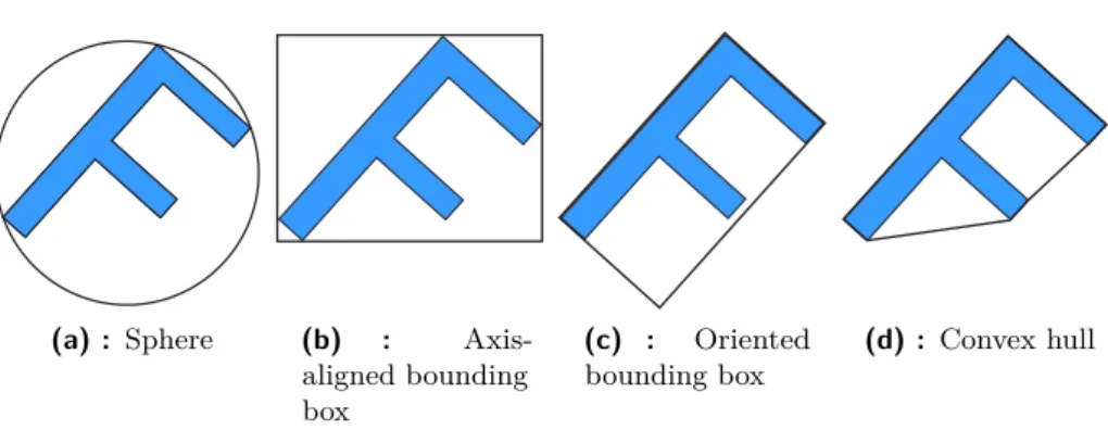
Many of collision detection algorithms have been proposed recently [19]. A widespread method used in many collision detectors is calledbounding volume hierarchy [20]. Suppose two non-convex objects, the robot and obstacle. The objects are decomposed into trees Tr and To, where a root of each
tree is the whole object and each node represents a bounded subset of the object. Possible bounding regions are shown in Figure 2.3. An intersection is first tested between the root nodes and if no exist, the algorithm reports no collision. If the bounding overlap, the algorithm recursively tests their children until it finds the intersection or reaches leaves of the tree. In that case, each polygon pair of the robot and obstacle is tested.
(a) : Sphere (b) :
Axis-aligned bounding box
(c) : Oriented bounding box
(d) : Convex hull
Figure 2.3: Possible bounding regions for the bounding volume hierarchy
...
2.3. Motion Planning2.3
Motion Planning
Generally, the motion planning is defined for a set that contains:
.
world W, either W =R2 orW =R3,
.
obstacle region O ⊂ W,.
semi-algebraic rigid robotA ⊂ W or a collection of mjoined segmentsA1, ...,Am⊂ W,
.
state space X,.
set of possible inputs U,.
initial state xI ∈ X,.
goal state xG or set of goal statesXgoal⊂ X.The motion planning executes a probing of the state space. A goal is to find a valid non-colliding path for the robot A in the world W from the initial position and velocity encoded by x1 to the goal region Xgoal. The
robot must obey geometric constraints given by obstacles and differential (non-holonomic) constrains given by the robot’s design. It was shown that the problem of motion planning is PSPACE-hard [21]. We can classify motion planning problems into three groups by constraints.
Holonomic planning The most basic motion planning is called holonomic
planning. The term refers to holonomic constraints. Holonomic constraints are constraints which reduce the number of DOF of the robot. Holonomic constraints appear in the formhi(q) = 0 and thusigeneralized coordinates
are blocked for the control. See Figure 2.4 for an example.
Non-holonomic planning This planning addresses problems with
non-integrable velocity constraints [22]. These constraints are common in systems that involve rotating parts like wheeled-robots (car) or aerial systems (aircraft, UAV3). Non-holonomic constraints are the constraints in the formgi(q,q˙) = 0.
It prevents to control all DOF separately since a change of the one coor-dinate might change others coorcoor-dinates as well. This is a difference with the holonomic planning, where all coordinates can be controlled separately. See Figure 2.5 for an example. Both holonomic and non-holonomic planners perform a search in the configuration space.
Kinodynamic planning The title refers to kinematic and dynamic
con-straints. Besides position and velocity constraints, acceleration constraints are present in this planning yielding equations ki(q,q,˙ q¨) = 0 [23]. Since
acceleration constraints exist, space to be searched is the full state space X.
2. Problem Analysis
...
Further in the thesis, we address all problems as probing of the state space regardless of a type even though we defined a state as x= (q,q˙). For holonomic and non-holonomic planning, one can assume x = q and hence
X =C.
Figure 2.4: A holonomic system, planar pendulum, with constraint in the form
x2+y2=l2that reduces the number of DOF. This system can be described by
one coordinateθ and henceq=θ andx= (θ,θ˙).
Figure 2.5: A car representing the non-holonomic system. A configuration of
Chapter
3
State of the Art
This chapter gives a brief overview of motion planning methods. There are three main approaches to motion planning algorithms different in the representation of the state space. The oldest group of algorithms is com-binatorial planning [24, 25]. The next group are artificial potential field
methods [26, 27]. At present, intensive research is ongoing in the field of
sampling-based planning [28].
Since the title of this thesis is Sampling-based motion planning for 3D rigid objects, we study sampling-based algorithms in more detail and Chapter 4 is devoted to the most important algorithm for the work.
3.1
Combinatorial Planning
In the task of probing the state space, the continuous space needs to be discretized. This can be done by several techniques. Combinatorial planning directly represents the free state space as a roadmap. The roadmap is an undirected graph G(V, E) in Xf ree, where vertices from the set V are states
fromX and edges from the setE are possible transitions between the states. After the roadmap is done, a graph search algorithm (A*,D*) is applied to find the shortest path.
The combinatorial planning requires polygonal obstacles O in order to create the roadmap representation of W. Because the motion planning operates in the state space X and not in the worldW, the obstacles need to be first transformed intoX to make Xobs. It is a very demanding task and exact transformation can be done only in simple problems, for example a 3D world with a rigid robot restricted only to the translation movement. In this cases, Xobs can be constructed as Xobs = O ⊕ −A(0), where ⊕is a special
3. State of the Art
...
Figure 3.1: The visibility graph
convolution called aMinkowski sum defined as
A⊕B={~a+~b|~a∈A,~b∈B}. (3.1) Let A(q)⊂ W define all points of the geometry of the robotAlocated in the configurationq.
The combinatorial algorithms are capable of solving easier planning prob-lems very elegant and intuitive. They are unfortunately limited by the low number of DOF and only holonomic constraints. On the other hand, their advantage is that they arecomplete1. For example, the 2D world with a robot moving only translationally is a great occasion to employ a combinatorial planner.
Visibility graph The roadmap is constructed by connecting mutually
visible vertices of obstacle polygons [29]. First, the initial and goal positions are connected to the all visible vertices of obstacles and world. Each vertex is then connected with others vertices if they are in sight. After this procedure, the roadmap looks like it is shown in Figure 3.1.
The visibility graph method finds an optimal path every time, but the path is close to obstacles. A naïve algorithm for construction the visibility graph has a time complexity O(n3) and the best algorithm is O(n2) [30].
Voronoi diagram The Voronoi diagram is a planar structure that partition
a plane into regions based on the distance of given points. The Voronoi region
Vk of a pointxk is defined as
Vk ={p∈ Xf ree| ∀i6=k, ρ(p, xk)≤ρ(p, xi)}, (3.2)
wherexi, xk are the input points and ρ is a metric. The Voronoi diagram is
formed from vertices that have the same distance from two or more points 1
Complete algorithm – Algorithm either finds a solution or reports that a solution does not exist.
...
3.1. Combinatorial Planning 0 0 0 0 0 0 0 0 0 0 0(a) : Voronoi regions
0 0 0 0 0 0 0 0 0 0 0
(b) : The found path
Figure 3.2: The Voronoi diagram with points representing obstacles
(see Figure 3.2). Edges are connections of the closest vertices. Edges of the diagram can be generated between two points, point and edge and between two edges (segment Voronoi diagram) which is useful for the motion planning since the obstacle boundary is represented by edges.
Voronoi diagrams have been well studied in the mobile robotics [31]. Con-struction of the Voronoi diagram is very fast (time complexityO(nlog(n)) in simple maps [32]), but it is not suitable for open spaces because the robot is attracted to the middle and sub-optimal paths are created.
Cell decomposition The idea of this algorithm is decomposing Xf ree
into cells with the specified shape. In each cell, which does not include the obstacle, is placed a vertex of the roadmap called adjacency graph. Edges of the adjacency graph are lines connecting the adjacent vertices. There are two versions of the cell decomposition algorithm: exact decomposition [33] and
approximate decomposition [34].
In the exact decomposition, space is decomposed into sets of variously large trapezoids or triangles. The cells may be constructed by cutting the space vertically from each polygon vertex as shown in Figure 3.3. Then, the
3. State of the Art
...
Figure 3.4: The approximate cell decomposition
vertex is placed in each segment border and inside each segment, for example to the center of the segment. The best-known algorithm for the exact cell decomposition has complexityO(nlog(n)).
The approximate decomposition is different in a mechanism of constructing the cells. All cells are the same simple shape, most often squares, creating a grid. Cells that intersect with the obstacles are removed. A solution existence depends on density of the grid. The algorithm starts with small density and then refines the density until it finds a solution (which may not exist). Thus, the algorithm is incomplete but easy to implement. See Figure 3.4 for the approximate cell decomposition in a simple environment.
3.2
Potential Fields
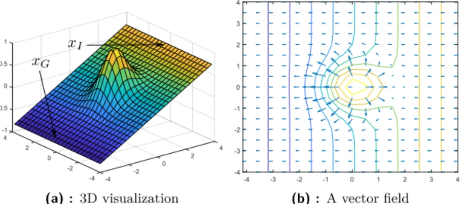
So far, achievable states of the robot were represented by a graph. Another approach for the holonomic or non-holonomic planning is to define an artificial potential field U(q) similar to the electric potential [26, 27]. The robot acts like a charged particle in the electric field and is attracted by a force
F=−∇~U(q). (3.3)
U(q) is modelled to has a global minimum at the goal state and a local maximum at the initial state. The goal generates the attractive potential that pulls the robot toward the goal. On the contrary, obstacles generate the repulsive potential that pushes the robot away from them (see Figure 3.5).
The disadvantage of the potential field methods is that the robot can get stuck in a local minimum that is not in at the goal. This can be resolved by using an optimization algorithm such as simulated annealing. Potential fields are commonly used for local motion planning2.
...
3.3. Sampling-based Planning -1 4 -0.5 2 4 0 2 0.5 0 1 0 -2 -2 -4 -4 (a) : 3D visualization -4 -3 -2 -1 0 1 2 3 4 -4 -3 -2 -1 0 1 2 3 4 (b) : A vector fieldFigure 3.5: A potential field of the space with one obstacle in the middle
Potential fields which represent the environment can be obtained at the start of the planning process or iteratively. The sequential approach computes the potential field on a grid. Before the algorithm starts, the continuous space must be discretized over a mesh with defined proportions.
3.3
Sampling-based Planning
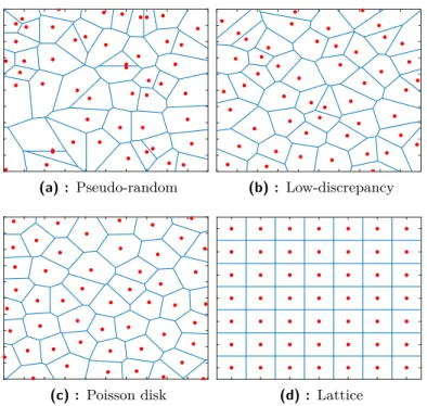
A sampling-based approach to the motion planning is based on representing the free space as a roadmap of sampled states. Sampling scheme generates random samples in the space. Whenever there exists a collision-free path between two samples, they can be connected by a line. Computation of the line shape is a task for the local planner. Examples of uniform sampling schemes are shown in Figure 3.6. Besides the most used uniform sampling, there are others techniques for the space sampling [35, 36].
The main difference with the probabilistic planning is that there is no need to explicit constructXobs before the algorithm starts. Sampling-based algorithms probe X without knowing anything about the world. They are independent of the geometrical representation of the world. It is possible due to the collision detection algorithm (see Section 2.2). This makes the collision detector the most critical part of the sampling-based planning.
The major advantage of sampling-based algorithms is the ability to solve all kinds of planning problems with non-holonomic or kinodynamic con-straints [37] with a low computational cost. Moreover, they can handle high DOF spaces and a wide variety of geometrical models. There are also modifications capable of planning in dynamic environments [38].
It has been proposed two basic sampling-based algorithms and many improved ones. The first sampling-based algorithm introduced in 1996 by
Jean-3. State of the Art
...
(a) : Pseudo-random (b) : Low-discrepancy
(c) : Poisson disk (d) : Lattice
Figure 3.6: Uniform sampling schemes with the Voronoi diagram representing
the scatter of random points
Claude Latombe and his collaborators3 is calledProbabilistic Roadmaps [14]. The other algorithm was introduced in 1998 by Steven M. LaValle. This algorithm is called Rapidly exploring Random Trees[12].
3.3.1 Probabilistic Roadmaps
Probabilistic Roadmaps (PRM) [14], as the title suggests, is a method for the motion planning similar to the combinatorial planning methods in terms of the algorithm proceeding. The algorithm is separated into two phases: learning phase andquery phase. In the learning phase, a roadmap is constructed by generating random samples (states) inX (Algorithm 1). The learning phase is followed by the query phase, where the task is to find a collision-free path between initial and goal states by a graph search algorithm.
The roadmap is represented by an undirected graphG= (V, E), where V
stands for vertices and E for edges. The vertices represent states and the edges represent transitions between two states given by a local planner. The graph is first composed of several connected components. As the algorithm continues, the number of connected components reduces until there is only one connected component left. The construction of PRM is shown in Figure 3.7 and examples of different roadmaps in Figure 3.8.
...
3.3. Sampling-based PlanningAlgorithm 1 Basic PRM - learning phase
Require: Initial state xI, number of iterations K, maximal distance of
neighbours d
Ensure: Undirected graphG
1: G.add_vertex(xI) 2: fork= 0toK do 3: xrand←RANDOM_STATE() 4: G.add_vertex(xrand) 5: N ←NEIGHBOURS(xrand, G, d) 6: for eachx∈N do 7: u←SELECT_INPUT(xrand, x) 8: if xis feasible then 9: G.add_edge(xrand, x, u) 10: return G
Given a state spaceX, initial state xI, distance dand empty graph G, the
algorithm proceeds as follows:
..
1. Learning phase Add the initial state to the graphG...
2. Generate a random statexrand∈ Xf ree and add it to the graph...
3. Select all neighbour states ofxrand within the distancedin terms of themetricρ.
..
4. For all the neighbours select a control input u ∈ U that ensures a collision-free transition and also minimizes a distance fromxrand to theneighbour.
..
5. If such a control input is found, add the neighbour to the graph...
6. If the roadmap is completed, go to step 7. Go to step 2 otherwise...
7. Query phase Employ a graph search algorithm to find a path in Gfrom xI toxG.
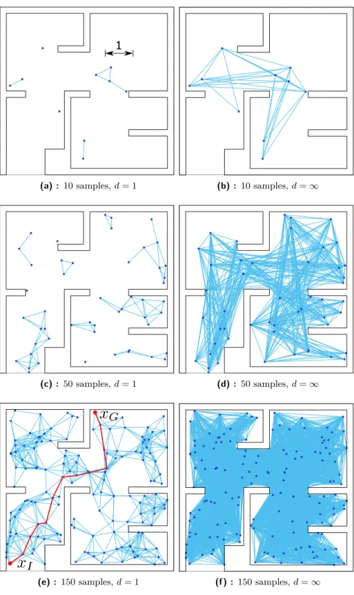
Figure 3.7: The construction of PRM, wherexrand is a randomly generated
point fromXf reeanddis the maximal distance to other points needed to make a connection.
3. State of the Art
...
1
(a) : 10 samples,d= 1 (b) : 10 samples,d=∞
p
(c) : 50 samples,d= 1 (d) : 50 samples,d=∞
(e) : 150 samples,d= 1
p
(f ) : 150 samples,d=∞
Figure 3.8: PRM with different number of samples and parameterd. With the
increasing number of samples, the uniform coverage of the space is achieved. (e) shows a computed path in the query phase.
Chapter
4
Rapidly Exploring Random Trees
Rapidly exploring Random Trees (RRT) [12, 13] is an effective sampling-based planning algorithm designed for handling various motion planning problems. The collision-free samples are saved in a treeT. In contrast with a common graph in case of PRM, the tree is an undirected graph without cycles. The absence of the cycles implies that every vertex in the tree has only one parent and thus no graph search algorithm is needed. It is possible to trace back nodes from the goal node to the initial node in order to find a path.
Although RRT is capable of probing high dimensional spaces with all kinds of constraints, it may be inappropriate for some planning problems. For example, the worlds with obstacles close together decrease the performance and efficiency of the algorithm. The parts with little space for passing the configuration are called narrow passages (see Figure 4.1). The basic RRT samples the space by a pseudo-random generator yielding in a lack of uniformity of the distribution. The analysis of weaknesses of the random sampling is shown in [39]. Improved versions of RRT, proposed to solve different types of problems, are also discussed in this chapter.
(a) : Hedgehog in the cage (b) : A tunnel
4. Rapidly Exploring Random Trees
...
4.1
Basic RRT
The first version of RRT was proposed in 1998. Introduction of RRT was a breakthrough in the motion planning due to the algorithm rapidity and ability to easy enhance the method. Unlike the combinatorial algorithms and PRM, RRT was designed to handle non-holonomic and kinodynamic planning. The non-holonomic version is described in Algorithm 2.
Given a state spaceX, initial state xI, time interval ∆tand empty treeT,
the RRT algorithm proceeds as follows:
..
1. Add the initial state to the treeT...
2. Generate a random statexrand∈ X...
3. Select the nearest neighbour ofxrand laying in T in terms of metricρ.Denote it xnear.
..
4. Select a control inputu∈U that ensures a collision-free transition and also minimizes a distance from xrand toxnear...
5. Apply the input u toxnear and compute a new state xnew. This stateis determined by integration of state equation ˙x=f(x, u) over a time interval ∆t.
xnew=xnear+ Z ∆t
0
f(x, u) dt (4.1)
..
6. If xnew is reachable by a collision-free path, add it to the tree. Ignore itotherwise.
..
7. Go to step 2.There are two key components in RRT and others sampling-based algo-rithms, and that is the NEAREST_NEIGHBOUR function and the collision detector. The task of the first one is to find the nearest vertex of another vertex. This is dependent on a choice of the metric. It can be performed by a KD-tree approach [40]. See [41] for a library ANN by David M. Mount,
Algorithm 2 Basic RRT
Require: Initial state xI, number of iterationsK, time interval ∆t
Ensure: RRT tree T
1: T.add_vertex(xI)
2: fork= 0toK do
3: xrand←RANDOM_STATE()
4: xnear ←NEAREST_NEIGHBOUR(xrand,T) 5: u←SELECT_INPUT(xrand, xnear)
6: xnew←NEW_STATE(xnear, u,∆t) 7: if xnew is feasiblethen
8: T.add_vertex(xnew) 9: T.add_edge(xnew, xnear, u)
...
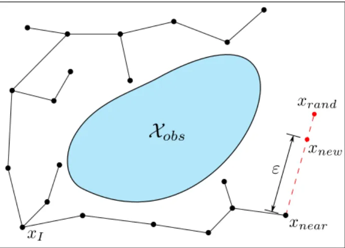
4.1. Basic RRTFigure 4.2: The construction of holonomic RRT.εdenotes the maximal distance
between two nodes.
Sunil Arya and [42] for the improved implementation called MPNN by Anna Yershova and Steven M. LaValle. The advantage of MPNN is a possibility to add nodes to the KD-tree while running. An approximate approach of determining the nearest neighbours is possible as well [43].
The collision detection system was briefly introduced in Section 2.2. The collision detector determines whether a new node is in a collision-free configu-ration. Two libraries frequently used in the motion planning are RAPID [44] and OZCollide [45] for their great usability. Both libraries are based on the method bounding volume hierarchy. An input to the libraries is apolygon soup, which is a group of unlinked polygons (most often triangles).
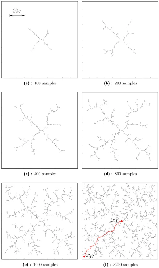
The tree tends to explore yet unexplored portions, so it leads to the uniform coverage of the space, as it can be seen in Figure 4.3. After crossing a threshold, let’s say 1600 samples in Figure 4.3, when the tree is spread out all over the space, the expansion stops and the tree is getting denser as the algorithm is running. This fact can be viewed as a ration betweenexploration
and exploitation [46]. Planning algorithms may be classified according to this ratio. Generally, the state space is infinitely large, but for real-world applications, we can assume the bounded state space by reachable positions and velocities. See figure 4.2 for an illustration of constructing RRT.
In the following picture, it is demonstrated a tree growing from the centre for a holonomic non-steerable system. Since a state in the holonomic planning does not contain any dependence on the previous state, the state transition equation is reduced to ˙x = f(u). For a non-steerable system, the input represents a bounded geodesic1 (|u| < ε), where ε denotes the maximal distance between two nodes. Moreover, it is shown a computed path between two selected nodes in Figure 4.3 (f).
1
Geodesic – The shortest route between two points. For Euclidean geometry it is a straight line.
4. Rapidly Exploring Random Trees
...
0 0 0 0 0 0 0 0 0 0 0 (a) : 100 samples 0 0 0 0 0 0 0 0 0 0 0 (b) : 200 samples 0 0 0 0 0 0 0 0 0 0 0 (c) : 400 samples 0 0 0 0 0 0 0 0 0 0 0 (d) : 800 samples 0 0 0 0 0 0 0 0 0 0 0 (e) : 1600 samples 0 10 20 30 40 50 60 70 80 90 100 0 0 0 0 0 0 0 0 0 0 0 (f ) : 3200 samplesFigure 4.3: The RRT tree growing from the centre for a small holonomic square
...
4.2. RRT-based Planners4.2
RRT-based Planners
Since the basic RRT planner does not produce optimal results for some planning problems, it has been developed hundreds of enhanced RRT-based planners to employ for specific problems. See [28] for an overview.
The first parameter of RRT that can be altered is the sampling strategy. In the basic RRT, the space is sampled by the uniform pseudo-random number generator. Other possible variants are: the intelligent sampling, biasing sampling, sampling around obstacles, sampling in narrow regions, hybrid sampling and more. Another important parameter is a metric. In general, a metric can represent an arbitrary parameter describing a cost of the transition from one state to another. Different metrics are used among the RRT-based algorithms.
Some algorithms modify the expansion step for better behaviour in highly constrained environments and narrow passages. For the purpose of finding an optimal (shortest, fastest) path, a whole group of optimal RRT-based algorithms exists. Moreover, there are improvements which apply a post-processing to a given path. They can smooth the path or make it shorter.
But first, let’s explore the group of algorithms which utilize more that one tree that grows from the beginning.
4.2.1 Multiple Trees
The idea is maintaining multiple trees instead of one tree rooted in the initial state in RRT. There is a basic variant with two trees calledRRT-Connect [47]. Some of the multiple trees methods even utilize more than two trees, namely three [48] or even more trees as required by the environment [49]. A common characteristic of these algorithms isheuristicwhich connects the trees whether it is possible. In experiments, it was shown that for some applications multiple trees are more efficient than a single tree [47].
RRT-Connect was the first multi-tree algorithm for the holonomic planning proposed just two years after the introduction of RRT in 2000 by Steven M. LaValle and James J. Kuffner. The algorithm was designed for problems that do not contain differential constraints. This approach is sometimes called a balanced bidirectional search. It is bidirectional because it involves two trees growing from two directions and balanced in order to keep their rapid exploring property.
Generally, the tree balancing is a part of the multi-tree algorithms, but not all algorithms involve it (RRT-Connect). In the case of the algorithm where the balancing is not present, it can almost lead to the basic RRT in
4. Rapidly Exploring Random Trees
...
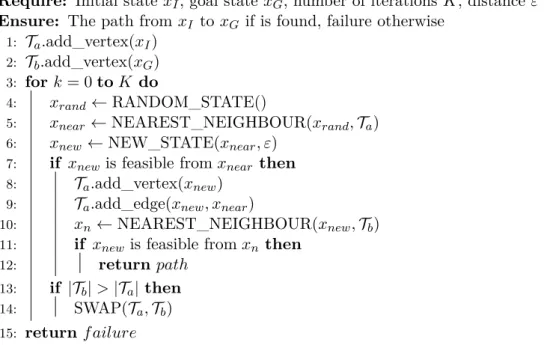
Algorithm 3 Balanced bidirectional RRT
Require: Initial statexI, goal statexG, number of iterations K, distanceε
Ensure: The path fromxI toxG if is found, failure otherwise
1: Ta.add_vertex(xI) 2: Tb.add_vertex(xG)
3: fork= 0toK do
4: xrand←RANDOM_STATE()
5: xnear ←NEAREST_NEIGHBOUR(xrand,Ta) 6: xnew←NEW_STATE(xnear, ε)
7: if xnew is feasible fromxnear then 8: Ta.add_vertex(xnew)
9: Ta.add_edge(xnew, xnear)
10: xn←NEAREST_NEIGHBOUR(xnew,Tb) 11: if xnewis feasible fromxnthen
12: return path
13: if |Tb|>|Ta|then
14: SWAP(Ta,Tb)
15: return f ailure
some environments, because one tree is strongly expanded while the other tree contains few nodes. The balancing can be realized by comparison the number of nodes in the trees or the total length.
Balanced bidirectional RRT starts by adding the initial state xI to the
tree Ta. The goal state xG is added to the second tree Tb. Then it picks
a random state xrand fromX, selects the nearest neighbour ofxrand in the
tree Ta and determines a new statexnew according to the maximal distance
between two nodes ε. Then, it is established if xnew is reachable from xnear
by a collision-free path. If so, xnew and u are recorded to Ta. The nearest
neighbour of xnew in the second treeTb is selected (xn). Ifxn and xnew can
0 0 0 0 0 0 0 0 0 0 0
Figure 4.4: Balanced bidirectional RRT rooted in the initial node and goal
...
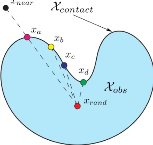
4.2. RRT-based PlannersFigure 4.5: The retraction step performs iterative optimization. The tree is
expanded toward the nodes xa, .., xd∈ Xcontact with the RRT expansion.
be connected by a collision-free path, the algorithm stops and returns a path (see Figure 4.4). If not, the trees are either swapped or not depending on the balance condition (Algorithm 3 – line 13). Then the loop starts again until a solution is found or the number of iterations expires.
4.2.2 Modification of the Extension Step
The extension step of the basic RRT is as simple as possible: for a given state xrand, determine the nearest neighbour xnear and apply the control
input toxnear. A new nodexnew is obtained by this procedure. The tree is
expanded toward xrand. The described expansion step is good enough for
simple problems but struggles in spaces with narrow passages. With high probability, a lot of nodes have to be added to the tree until one of the nodes will be situated in the narrow passage.
Modifications of the extension step improve the usability of RRT in narrow passages. The first algorithm to be discussed isRetraction-based RRT [50].
Retraction-based RRT This algorithm proceeds the same as the
holo-nomic RRT untilxnewdoes not lie inXobs. In that case, basic RRT ignores the
new node and generates a new one. Retraction-based RRT runs aretraction step which determines the closest point to the parent such that the point lies on an obstacle boundary. The retraction step is an optimization problem defined as
xm = arg min x∈Xcontact
ρ(x, xrand), (4.2)
where xrand is a given colliding state, ρ is the metric and Xcontact ⊆ Xobs
boundary of obstacles called thecontact space. See Figure 4.5 for an illustra-tion of the retracillustra-tion step.
4. Rapidly Exploring Random Trees
...
Algorithm 4 Retraction-based RRT
Require: Initial state xI, number of iterationsK, distance ε
Ensure: RRT tree T
1: T.init(xI)
2: fork= 0toK do
3: xrand←RANDOM_STATE()
4: xnear ←NEAREST_NEIGHBOUR(xrand,T) 5: xnew←NEW_STATE(xnear, ε)
6: if xnew is feasiblethen 7: T.add_vertex(xnew) 8: T.add_edge(xnew, xnear, u)
9: else
10: S ←RETRACTION(xrand, xnear)
11: for each xi ∈S do
12: STANDARD_RRT_EXPANSION(T, xi)
13: return T
Given a colliding statexrand and its nearest neighbourxnear, the retraction
step proceeds as follows:
..
1. Projectxnear intoXcontact to generate a new samplexa...
2. Perform acontact query by computing new samples around xa, whichhave a minimal distance between the robot and obstacle.
..
3. Search the samples computed by the contact query and determine a new sample xb inXcontact, which locally minimizes the distance to xrand. Ifthe new samplexb satisfy ρ(xb, xrand)< ρ(xa, xrand), continue to step 4.
End the algorithm otherwise.
..
4. Assign xnear =xb and go to step 1.The RETRACTION(xrand, xnear) function assigns all samples xa, xb, ...
given by the retraction step to a set S. The standard expansion from the basic RRT is performed for all nodes from the setS (line 12 in Algorithm 4). Thus, the tree expands around the obstacles and the performance in narrow passages is highly increased.
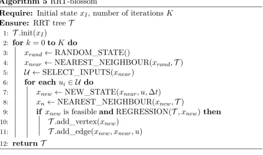
RRT-blossom Another example of a method with the modified extension
step is RRT-Blossom [51]. The algorithm is specific by a local flood-fill behaviour. This mechanism helps RRT-blossom to escape a local minimum, where the robot may get stuck, in highly constrained environments. RRT-blossom is well employable for non-holonomic and kinodynamic problems.
RRT-blossom starts, just like Retraction-based RRT, same as the basic RRT. It generates a random state xrand and finds its nearest neighbour
xnear in terms of the metric ρ. Then, control inputs ui are assigned to a
set U. The inputs are chosen by the function SELECT_INPUTS(xnear)
...
4.2. RRT-based PlannersAlgorithm 5 RRT-blossom
Require: Initial state xI, number of iterationsK
Ensure: RRT treeT
1: T.init(xI)
2: fork= 0toK do
3: xrand←RANDOM_STATE()
4: xnear ←NEAREST_NEIGHBOUR(xrand,T) 5: U ←SELECT_INPUTS(xnear)
6: for eachui∈ U do
7: xnew ←NEW_STATE(xnear, u,∆t) 8: xn←NEAREST_NEIGHBOUR(xnew,T)
9: if xnewis feasibleandREGRESSION(T, xnew) then 10: T.add_vertex(xnew)
11: T.add_edge(xnew, xnear, u)
12: return T
inputs from U ∈U to xnear. If xnew is feasible and theregression function
REGRESSION(T, xnew) returns true, xnew is added to the tree T.
The regression function is an important technique in RRT-blossom. It ensures the rapidly exploring property of the RRT algorithm by eliminating nodes which tend to regress as it is shown in Figure 4.6. Generally, implement-ing the regression function is a demandimplement-ing task. For holonomic applications, this task is greatly simplified and we can effectively compute the regression only with knowledge of the distance metric ρ as
REGR.(T, xnew) = (
FALSE if∃x∈ T |ρ(x, xnew)< ρ(xnear, xnew)
TRUE otherwise .
(4.3) The regression function from Equation 4.3 returns TRUE only if no node from T is closer toxnew than the parent and therefore ifxn=xnear.
Figure 4.6: RRT-blossom adds nodesxnew3, xnew5, xnew7 to the tree. Other
nodes are excluded by the regression function because their nearest neighbour is notxnear.
4. Rapidly Exploring Random Trees
...
(a) : Select the best parent (b) : Rewire the tree
Figure 4.7: RRT* performing the optimization of the tree
4.2.3 Optimal Planning
Disadvantage of all basic sampling-based methods is a non-optimal output path. This issue can be solved by utilizing an optimal RRT-based planner called RRT* [52] introduced by Sertac Karaman and Emilio Frazzoli in 2011. It has been proven that the paths computed by RRT* have the asymptotically optimal property [52] and therefore RRT* always finds the shortest path in the infinite amount of time.
The optimal property of RRT* is redeemed by a longer computation time compared with the basic RRT. The longer computation time is caused by a feature called rewiring which improves the path quality as the algorithm runs. The original algorithm is limited to holonomic problems only.
Since the first optimal RRT-based algorithm was introduced, many new relevant RRT*-based algorithms have been proposed. We can name a non-holonomic expansionAnytime RRT* [53] by the same authors as the original RRT*, memory efficient version RRT*FN [54] or a version with the smart sampling Informed RRT* [55]. A complete survey on RRT*-based methods is presented in [56].
Before we will discuss RRT*, it is necessary to present functions used in Algorithm 6. For two given statesxa, xb ∈ RN, LINE(xa, xb) is a function
xa, xb→Rthat denotes a path length fromxa toxb. Let COST(xa) denote a
function xa→R, that returns a distance ofxa to the beginning when passing
by a path. This definition implies that COST(xI) = 0. Let PARENT(xa)
be a function xa → xb that returns a parent node of xa. With respect to
the previous definitions, we can write COST(xa) = COST(PARENT(xa)) +
...
4.2. RRT-based PlannersAlgorithm 6 RRT*
Require: Initial state xI, number of iterationsK, distanceε
Ensure: RRT* treeT
1: T.init(xI)
2: fork= 0toK do
3: xrand←RANDOM_STATE()
4: xnear ←NEAREST_NEIGHBOUR(xrand,T) 5: xnew←NEW_STATE(xnear, ε)
6: if xnew is feasiblethen 7: T.add_vertex(xnew)
8: Xnear←NEIGHBOURS(xnew,T,min{γ(log|T |/|T |)1/N, η})
9: xmin ←xnear
10: cmin ←COST(xnear) + LINE(xnear, xnew)
11: for each xn∈Xnear do
12: if xnis feasible fromxnew andCOST(xn)+LINE(xn, xnew)<
cmin then
13: xmin←xn
14: cmin ←COST(xn) + LINE(xn, xnew) 15: T.add_edge(xnew, xn)
16: for each xn∈Xnear do
17: if xn is feasible from xnew and COST(xnew) +
LINE(xn, xnew)<COST(xn) then
18: xparent←PARENT(xn)
19: T.remove_edge(xn, xparent) 20: T.add_edge(xn, xnew)
21: return T
Given an initial state xI, empty treeT and state spaceX, RRT* proceeds
as follows:
..
1. Holonomic RRT Add the initial state to the tree T...
2. Generate a random statexrand∈ X...
3. Select the nearest neighbour of xrand in terms of metric ρ. Denote itxnear.
..
4. Determine a new statexnew by connectingxrand toxnear by a straightline. If LINE(xrand, xnear) < ε, then xnew ← xrand. Compute a state
that satisfy LINE(xnew, xnear) =εand lie on the line otherwise.
..
5. Ifxnew is reachable by a collision-free path, add it to the tree. If not,ignore it and go to step 2.
..
6. Best parent Select all neighbours of xnew within the distancemin γ log|T | |T | N1 , η (4.4) whereγ and η are parameters dependent on the environment,|T | is the number of nodes in the tree andN is the number of dimensions.
4. Rapidly Exploring Random Trees
...
..
7. Cycle through all the neighbours and find the parent of xnew with aminimum-cost path to the initial node among them.
..
8. Rewiring Cycle again through all the neighbours and if a path to thenode throughxnewis shorter, remove the existing connection to its parent
and add the new less costly connection. Assign xnew as the new parent.
See Figure 4.7 for an illustration of the rewiring procedure.
0 0 0 0 0 0 0 0 0 0 0 (a) : RRT - Environment 1 0 0 0 0 0 0 0 0 0 0 0 (b) : RRT* - Environment 1 0 0 0 0 0 0 0 0 0 0 0 (c) : RRT - Environment 2 0 0 0 0 0 0 0 0 0 0 0 (d) : RRT* - Environment 2
Figure 4.8: Comparison of RRT and RRT* for a holonomic robot. The path
Chapter
5
Our Contribution
This chapter is dedicated to our contribution to the motion planning. In the first section, we introduce a new algorithm for the holonomic motion planning based on the basic RRT. In the other section, our new algorithm RRT-sphere and other implemented RRT-based algorithms are tested by means of own 3D models and benchmark [15] for their execution time, number of explored nodes and length of the final path.
5.1
RRT-sphere
RRT-sphere is a novel RRT-based algorithm we propose to improve the performance of RRT in low constrained environments. Every discussed algorithm so far utilized uniform sampling scheme. Proposed RRT-sphere samples the state space by adaptive sampling which attracts the samples toward the goal state whether it is possible. The principle of the non-uniform sampling ensures that no redundant nodes are created and thus it saves system resources like RAM and CPU.
This method is designed to solve holonomic and non-holonomic problems, but we only focus on holonomic systems in the thesis. Testing RRT-sphere under non-holonomic constraints and automatic tuning of parameters is a possible avenue for the future work.
Unlike the RANDOM_STATE() function from previous algorithms, the method for generating new samples is modified in RRT-sphere. RAN-DOM_STATE (xG, h) generates new states around the goal statexG within
the radius h. The part of the state space, where random samples xrand are
located, looks like N-D hypersphere with the centre in xG, where N is the
5. Our Contribution
...
Algorithm 7 RRT-sphere
Require: Initial state xI, goal state xG, number of iterations K, initial
radiush Ensure: RRT tree T 1: T.add_vertex(xI) 2: a, b←0 3: fork= 0toK do 4: if kmod α= 0 then 5: a←0 6: b←0 7: h←SET_RADIUS(a, b) 8: xrand←RANDOM_STATE(xG, h)
9: xnear ←NEAREST_NEIGHBOUR(xrand,T) 10: u←SELECT_INPUT(xrand, xnear)
11: xnew←NEW_STATE(xnear, u,∆t) 12: if xnew is feasiblethen
13: T.add_vertex(xnew) 14: T.add_edge(xnew, xnear, u)
15: a←a+ 1
16: else
17: b←b+ 1
18: return T
The radius changes dynamically according to the ratio of non-colliding and colliding nodes in the function SET_RADIUS(a, b), whereais the number of feasible nodes andb is the number of colliding nodes. The counters aand
b reset to 0 after the established number of iterations expires. The number of required iterations to reset the counter is denoted α. Let β denote the
stretching factor which represents the speed of expansion/shrinking of the area around xG (β ∈<0,1 >). Adaptation of the radius is shown in Figure 5.1.
The full pseudo-algorithm of RRT-sphere is shown in Algorithm 7. The function that controls change of the radius h is defined as:
SET_RADIUS(a, b) = h←h+βh ifk mod α= 0∧a < b h←h−β2h ifk mod α= 0∧a > b unchangedh otherwise (5.1)
Provided that there exists a path without majority of narrow passages from
xI to xG, RRT-sphere finds the path using a smaller amount of samples in
comparison with the original RRT and other RRT-based methods with the uniform probing of the space. This algorithm never produces worse results than the basic RRT because in the worst case,h is large enough to cover the all state space yielding in the uniform coverage.
...
5.2. Experimental Results 0 0 0 0 0 0 0 0 0 0 0 (a) : 40 iterations 0 0 0 0 0 0 0 0 0 0 0 (b) : 80 iterations 0 0 0 0 0 0 0 0 0 0 0 (c) : 140 iterations 0 0 0 0 0 0 0 0 0 0 0 (d) : 160 iterationsFigure 5.1: Changing of the radius hin RRT-sphere according to the number
of successfully added nodes. New nodes are generated in the red area.
5.2
Experimental Results
The experimental section of the thesis is divided into three parts. In the first part, we analyse RRT-sphere parameters α, β and their influence on the motion planning performance. Then, we perform experiments on various motion planning problems in 2D worlds with all implemented algorithms — RRT [12], Retraction-based RRT [50], blossom [51], RRT* [52], RRT-sphere, and in 3D worlds with three selected algorithms. The algorithms are compared in detail and results are provided in the section.
5.2.1 RRT-sphere Parameters
The correct initializing of parameters is the important preliminary phase of all sampling-based motion planning algorithms. Wrongly tuned parameters can lead to substandard quality of the planning. Internal constants of motion planning algorithms affect the run-time, memory requirement and quality of the final path. There exists a specific set of parameters which is optimal for the particular planning task and gives the best results. It is not possible to tune the parameters correctly without knowledge of the environment.
5. Our Contribution
...
0.1 0.2 0.3 0.4 0.5 0.6 0.7 0.8 0.9 1 10 20 30 40 50 60 70 80 90 100 370.6 367.6 413 373.6 397.7 349.8 398.8 349.4 349.2 345.4 309.9 324.5 403.7 424.6 412.7 398.8 461.6 340.2 400.3 439.7 308.5 346.8 350.5 409.8 395.1 399.2 456.9 417.5 375.4 327.6 319.8 344.6 344.1 366.1 429.6 447.6 362.6 310.3 309.7 327.3 400.5 358.1 408.3 374.1 388.9 319.7 340.6 350.7 327.3 336.1 355.8 439.9 308.2 320 318.9 308.2 359.2 369.2 313.9 316 335.2 351.4 354 347.2 322.4 343.4 317.5 308.1 305 322.5 325.1 356.4 279.4 262.8 288.4 254.2 275.3 237.5 283.1 267.3 230.6 249.8 287.3 221.5 238.8 275.4 287.8 303.4 221.7 245 241.1 290.3 292.9 304 228.7 235.3 257.5 270.2 288.9 300.3 250 300 350 400 450Figure 5.2: The dependency of RRT-sphere parametersαandβ on the number
of nodes required to find a path in the 2D map
0.1 0.2 0.3 0.4 0.5 0.6 0.7 0.8 0.9 1 10 20 30 40 50 60 70 80 90 100 1247 1050 1252 1186 1309 1056 1242 1498 1040 1414 1605 1010 1140 1308 1305 1173 1320 1304 1594 1045 1535 1239 1431 1429 1271 1424 1218 1226 1279 1034 1614 1143 1480 1078 1063 1596 1201 990.4 1468 1248 1369 1140 1220 1323 1620 1308 1245 1682 1517 1497 993.9 1627 1656 1357 989.2 1473 1485 1072 1295 1715 1313 1135 1722 1409 1293 1533 1272 1332 1654 1224 796.5 726.8 920.2 844.9 957 960.4 903.5 912 962.9 767.2 937.7 880.6 838.5 932.4 854.3 893.1 862.5 903 895.2 860.2 842.9 883.9 826.5 950.3 899.1 918.3 878 932.4 591.9 773.1 600 800 1000 1200 1400 1600
Figure 5.3: The dependency of RRT-sphere parametersαandβ on the number
...
5.2. Experimental Results(a) : The 2D map (b) : The 3D map
Figure 5.4: Two testing maps utilized for evaluating RRT-sphere parameters
with calculated paths
The maps used for testing the dependency of RRT-sphere parameters on the planning quality are shown in Figure 5.4. We determine the number of generated nodes until the algorithm finds a path. The parameter α is examined in the interval < 10,100 > and the parameter β in the interval
<0.1,1>. Results are visualised asheat maps in Figure 5.2 and Figure 5.3. The value in each box is the mean of ten tests. For comparison, the basic RRT generates 5000 nodes on average in the 2D map.
In the 2D map, there can be observed a strong correlation between the parameters and number of needed nodes to find a path. When the parameters approach closer to α = 10 and β = 0.1, the number of generated nodes reduces. Experiments in the 3D map do not exhibit the correlation. Best results in the 3D map are produced byα = 90 andβ = 0.8.
5.2.2 Experiments in 2D Environments
We perform experiments in 2D environments with the robot which is rep-resented by a square. The robot is capable of moving in two DOF and its configuration (state) isq= (x, y), wherexandy are translational coordinates. The system is holonomic and thus the robot can displace independently in both directions. The state space has dimensions 200 cm by 200 cm and the robot has dimensions 20 cm by 20 cm.
For the testing, we designed three maps: easy (1), obstacles (2) and L-trap (3) An assignment for the robot is to find a path from (0,0) to (200,200).
The step size is set to 3 for all algorithms. We utilized Euclidean metric. Examples of computed paths in all testing maps are shown in Figure 5.5.
5. Our Contribution
...
(a) : RRT (1) (b) : RRT (2) (c) : RRT (3)
(d) : Retr. RRT (1) (e) : Retr. RRT (2) (f ) : Retr. RRT (3)
(g) : RRT-blossom (1) (h) : RRT-blossom (2) (i) : RRT-blossom (3)
(j) : RRT* (1) (k) : RRT* (2) (l) : RRT* (3)
(m) : RRT-sphere (1) (n) : RRT-sphere (2) (o) : RRT-sphere (3)
Figure 5.