Runtime Measurements in the Cloud: Observing, Analyzing, and Reducing Variance

(1)

Runtime Measurements in the Cloud: Observing,

Analyzing, and Reducing Variance

J¨org Schad, Jens Dittrich, Jorge-Arnulfo Quian´e-Ruiz

Information Systems Group, Saarland University

http://infosys.cs.uni-saarland.de

ABSTRACT

One of the main reasons why cloud computing has gained so much popularity is due to its ease of use and its ability to scale computing resources on demand. As a result, users can now rent computing nodes on large commercial clusters through several vendors, such as Amazon and rackspace. However, despite the attention paid by Cloud providers, performance unpredictability is a major issue in Cloud com-puting for (1) database researchers performing wall clock ex-periments, and (2) database applications providing service-level agreements. In this paper, we carry out a study of the performance variance of the most widely used Cloud infras-tructure (Amazon EC2) from different perspectives. We use established microbenchmarks to measure performance vari-ance in CPU, I/O, and network. And, we use a multi-node MapReduce application to quantify the impact on real data-intensive applications. We collected data for an entire month and compare it with the results obtained on a local cluster. Our results show that EC2 performance varies a lot and often falls into two bands having a large performance gap in-between — which is somewhat surprising. We observe in our experiments that these two bands correspond to the dif-ferent virtual system types provided by Amazon. Moreover, we analyze results considering different availability zones, points in time, and locations. This analysis indicates that, among others, the choice of availability zone also influences the performance variability. A major conclusion of our work is that the variance on EC2 is currently so high that wall clock experiments may only be performed with considerable care. To this end, we provide some hints to users.

1. INTRODUCTION

Cloud Computing is a model that allows users to easily access and configure a large pool of remote computing re-sources (i.e. aCloud). This model has gained a lot of pop-ularity mainly due to its ease of use and its ability to scale up on demand. As a result, several providers such as Ama-zon, IBM, Microsoft, and Yahoo! already offer this

technol-Permission to make digital or hard copies of all or part of this work for personal or classroom use is granted without fee provided that copies are not made or distributed for profit or commercial advantage and that copies bear this notice and the full citation on the first page. To copy otherwise, to republish, to post on servers or to redistribute to lists, requires prior specific permission and/or a fee. Articles from this volume were presented at The 36th International Conference on Very Large Data Bases, September 13-17, 2010, Singapore.

Proceedings of the VLDB Endowment,Vol. 3, No. 1

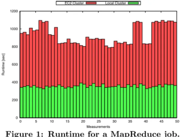
Figure 1: Runtime for a MapReduce job.

ogy. For many users, especially for researchers and medium-sized enterprises, the cloud computing model is quite at-tractive, because it is up to the cloud providers to maintain the hardware infrastructure. However, despite the attention paid by cloud providers, some cloud computing nodes may attain orders of magnitude worse performance than other nodes [12]. This indeed may considerably influence perfor-mance of real applications. For example, we show the run-times of a MapReduce job for a 50-node EC2 cluster and a 50-node local cluster in Figure 1. We can easily see that performance on EC2 varies considerably. There exist sev-eral reasons why such performance inconsistencies may oc-cur. In particular, contention for non-virtualized resources (e.g. network bandwidth) is clearly one of the main reasons for performance unpredictability in the cloud.

Performance unpredictability in the cloud is in fact a ma-jor issue for many users and it is considered as one of the major obstacles for cloud computing [12]. For example, re-searchers expect comparable performance for their applica-tions at any time, independent of the current workload of the cloud; this is quite important for researchers, because of repeatability of results. Another example are enterprises that depend onService Level Agreement(SLA), e.g. a Web page has to be rendered within a given amount of time. Those enterprises expect cloud providers to makeQuality of Service(QoS) guarantees. Therefore it is crucial that cloud providers offer SLAs based on performance features — such as response time and throughput. However, cloud providers typically base their SLAs on the availability of their offered services only [1, 2, 10].

Therefore, there is currently a clear need for users — who have to deal with this performance unpredictability — to better understand the performance variance in a cloud.

(2)

exhaustively evaluate the performance of Amazon EC2 — which is by far the most known and widely used cloud in-frastructure today. Our major contributions are as follows. 1. We perform our experiments at three different levels:

• single EC2 instances, which allows us to estimate the performance variance of a single virtual node,

• multiple EC2 instances, which allows us to esti-mate the performance variance of multiple nodes,

• different locations (US and Europe), which allows us to estimate the performance variance of differ-ent data cdiffer-enters in differdiffer-ent locations.

2. We provide an analysis of our results focussing on:

• distribution, mean, and coefficient of variation (COV) of the measurements,

• variance when increasing the size of a virtual clus-ter, i.e. increasing the number of virtual nodes,

• the impact of variance on the performance of a real application (MapReduce).

3. We identify that, performance can be divided in two bands and, among other factors, the virtual system type used by EC2 is a major source of performance variability. We also provide some hints to users to re-duce the performance variability of their experiments. Additionally, we show a decomposition of the variability by day, hour of the day, and weekday in Appendix A.

We expect this study to have a major positive impact in practice for three main reasons: (i) it helps researchers to better understand their results obtained from running experiments on Amazon EC2, (ii) it allows enterprises to better understand the QoS they get from Amazon EC2 and hence what they can offer to their end-users and (iii) it offers some hints on how to deal with this variance . To the best of our knowledge, this is the first work providing a performance study to such an extent.

This paper is structured as follows. We survey related work in Section 2. We provide a detailed view on Amazon EC2 in Section 3. We discuss, in Section 4, different inter-esting aspects when measuring the performance of EC2 and present the different benchmarks we use in our experiments. In Section 5, we present the results and provide in Section 6 a variability analysis of our results. Section 7 analyzes the impact of performance variability on larger clusters of vir-tual nodes and real applications. We then provide in Sec-tion 8 some advice to users in order to allow for meaningful experimental results and repeatability on EC2.

2. RELATED WORK

Cloud computing has been the focus of several research works and is still gaining more attention from the research community. As a consequence, many cloud evaluations have been done with different goals in mind. Armbrust et al. [12] mention performance unpredictability as one of the major obstacles for cloud computing. They found that one of the reasons of such unpredictability is that certain technologies, such as PCI Express, are difficult to virtualize and hence to share. Lenk et al. [21] propose a generic cloud computing stack with the aim of classifying cloud technologies and ser-vices into different layers, which in turn provides guidance about how to combine and interchange technologies. Binnig et al. [13] claim that traditional benchmarks (like TPC) are

not sufficient for analyzing the novel cloud services as they require static settings and do not consider metrics central to cloud computing such as robustness to node failures. Li et al. [22] discuss some QoS guarantees and optimizations for the cloud. Ristenpart et al. focus on security aspects and conclude that fundamental risks arise from sharing phys-ical infrastructure between mutually distrusful users [26]. Cryans et al. [14] compare the cloud computing technol-ogy with database systems and propose a list of comparison elements. Kossmann et al. [20] evaluate the cost and per-formance of different distributed database architectures and cloud providers. They mention the problem of performance variance in their study, but they do not evaluate it further. Other authors [17, 24] evaluate the different cloud services of Amazon in terms of cost and performance, but he does not provide any evaluation of the possible impact that per-formance variance may have on users applications. Dejun et al. [16] also study the performance variance on EC2, but they only focus on an application level (MySQL, Tomcat performance). Therefore, they do not provide detailed in-sight to the source of the performance variance issue.

Finally, new projects that monitor the performance of clouds have recently emerged. For example, CloudCli-mate [5] and CloudKick [6] already perform performance monitoring of different clouds. EC2 also offers Cloud-Watch [7] which provides monitoring forAmazon Web Ser-vicescloud resources. However, none of the above works fo-cuses on evaluating the possible performance variability in clouds or even give hints on how to reduce this variability.

There also exist a number of studies comparing the actual performance difference between cloud computing and tradi-tional high performance clusters so as to evaluate the ap-plicability of cloud computing to scientific applications [19, 23]. Nonetheless, they focus on the overall runtime and not on performance variability.

3. AMAZON EC2 INFRASTRUCTURE

The Amazon Elastic Computing Cloud (EC2) was not ini-tially designed as a cloud platform. Instead, the main idea at Amazon was to increase the utilization of their servers, which only had a peak around Christmas. When EC2 was released in 2006 it was the first commercial large scale pub-lic cloud offering. Nowadays, Amazon offers a wide range of cloud services besides EC2: S3, SimpleDB, RDS, and Elastic MapReduce. Amazon EC2 is very popular among researchers and enterprises requiring instant and scalable computing power. This is the main reason why we focus our analysis study on this platform.

Amazon EC2 provides resizable compute capacity in a computational cloud. This platform changes the economics of computing by allowing users to pay only for the ca-pacity that their applications actually need (pay-as-you-go model). The servers of Amazon EC2 are Linux-based vir-tual machines running on top of the Xen virvir-tualization en-gine. Amazon calls these virtual machines instances. In other words, it presents a true virtual computing environ-ment, allowing users to use web service interfaces to acquire instances for use, load them with their custom applications, and manage their network access permissions. Instances are classified into three types: standard instances (which are well suited for most applications), high-memory instances

(which are especially for high throughput applications), and high-cpuinstances (which are well suited for

(3)

compute-intensive applications). We consider small instances in our performance evaluation, because they are the default in-stance size and frequently demanded by users. Standard instances are classified by their computing power which is claimed to correspond to physical hardware:

(1.) small instance (Default), corresponding to 1.7 GB of main memory, 1 EC2 Compute Unit (i.e. 1 virtual core with 1 EC2 Compute Unit), 160 GB of local instance storage, and 32-bit platform;

(2.) large instance, corresponding to 7.5 GB of main mem-ory, 4 EC2 Compute Units (2 virtual cores with 2 EC2 Com-pute Units each), 850 GB of local instance storage, 64-bit platform;

(3.) extra large instance, corresponding to 15 GB of main memory, 8 EC2 Compute Units (4 virtual cores with 2 EC2 Compute Units each), 1690 GB of local instance storage, and 64-bit platform.

One EC2 Compute Unit is claimed to provide the “equiva-lent CPU capacity of a 1.0-1.2 GHz 2007 Opteron or 2007 Xeon processor” [2]. Nonetheless, as there exist many mod-els of such processors in the market, it is not clear what is the CPU performance any instance can get.

While some resources like CPU, memory, and storage are dedicated to a particular instance, other resources like the network and the disk subsystem are shared amongst in-stances. Thus, if each instance on a physical node tries to use as much of one of these shared resources as possible, each receives an equal share of that resource. However, when a shared resource is underutilized, it is able to consume a higher share of that resource while it is available. The per-formance of shared resources also depends on the instance type which has an indicator (moderate or high) influenc-ing the allocation of shared resources. Moreover, there exist currently three different physical locations (two in the US and one in Ireland) with plans to expand to other locations. Each of these locations contains different availability zones being independent of each other in case of failure.

4. METHODOLOGY

To evaluate the performance of a cloud provider, one can run typical cloud applications such as MapReduce [15] jobs, which are frequently excecuted on clouds, or databases ap-plications. Even though these applications are a relevant measure to evaluate how well the cloud provider operates in general, we also wanted a deeper insight of application per-formance. This is why we focus on a lower level benchmark and hence measure the performance of individual compo-nents of the cloud infrastructure. Besides a deeper under-standing of performance, measuring at this level also allows users to predict performance of a new application to a cer-tain degree. To relate these results to real data intensive applications, we analyze the impact of the size of virtual clusters on variance and the impact on MapReduce jobs. In the following, we first discuss the different infrastructure components and aspects we focus on and then present the benchmarks and measures we use in our study.

4.1 Components and Aspects

We need to define both the set of components of which we want to measure the performance and the way we want to carry out our study. In other words, we have to answer the following two important questions:

What to measure? We focus on the following components

that may considerably influence the performance of actual applications (we discuss benchmark details in Section 4.2).

1. Instance startupis important for cloud applications in order to quickly scale up during peak loads,

2. CPUis a crucial component for many applications, 3. Memory speedis crucial for any application, but it is

even more important for data-intensive applications such DBMSs or MapReduce,

4. Disk I/O (sequential and random)is a key component because many cloud applications require instances to store intermediate results on local disks if the input data may not be processed in main memory or for fault-tolerance purposes, such as MapReduce, 5. Network bandwidth between instancesis quite

impor-tant to consider because cloud applications usually process large amounts of data and exchange them through the network,

6. S3 access from outside of Amazonis important because most users first upload their datasets to S3 before run-ning their applications in the cloud.

How to run the measurements? For each of the

pre-vious components there are three important aspects that may influence the performance. First: Do small and large instances have different variations in performance? Second:

Does the EU location suffer from more variance performance than the US location? Do different availability zones impact performance? Third: Does performance depend on the time of day, weekday, or week?

In this paper, we study these three aspects and provide an answer to all these questions.

4.2 Benchmarks Details

We now present in more detail the different benchmarks we use for measuring the performance of each component.

Instance Startup. To evaluate this component, we

mea-sure the elapsed time from the moment a request for an instance is sent to the moment that the requested instance is available. To do so, we check the state of any starting instance every two seconds and stop monitoring when its status changes to “running”.

CPU. To measure CPU performance of instances, we use theUnix Benchmark Utility(Ubench) [11], which is widely used and stands as the definitive Unix synthetic benchmark for measuring CPU (and memory) performance. Ubench provides a single CPU performance score by executing 3 minutes of various concurrent integer and floating point cal-culations. In order to properly utilize multicore systems, Ubench spawns two concurrent processes for each CPU available on the system.

Memory Speed. We also use the Ubench benchmark [11]

to measure memory performance. Ubench executes random memory allocations as well as memory to memory copy-ing operations for 3 minutes concurrently uscopy-ing several pro-cesses. The result is a single memory performance score.

Disk I/O.To measure disk performance, we use Bonnie++

benchmark which is a disk and filesystem benchmark. Bon-nie++ is a c++ implementation of Bonnie [4]. In contrast to Ubench, Bonnie++ reports several numbers as results. These results correspond to different aspects of disk perfor-mance, including measurements forsequential reads, sequen-tial writes, andrandom seeks, in two main contexts: byte by

(4)

CPU Memory Sequential Read Random Read Network

[Ubench score] [Ubench score] [KB/second] [seconds] [MB/second]

Meanx 1,248,629 390,267 70,036 215 924

Min 1,246,265 388,833 69,646 210 919

Max 1,250,602 391,244 70,786 219 925

Range 4,337 2,411 1,140 9 6

COV 0.001 0.003 0.006 0.019 0.002

Table 1: Physical Cluster: Benchmark results obtained as baseline

byte I/Oandblock I/O. For further details please refer to [4]. In our study, we report results for sequential reads/writes and random reads block I/O, since they are the most influ-encing aspects in database applications.

Network Bandwidth. We use the Iperf benchmark [8]

to measure network performance. Iperf is a modern alter-native for measuring maximum TCP and UDP bandwidth performance developed by NLANR/DAST. It measures the maximum TCP bandwidth, allowing users to tune various parameters and UDP characteristics. Iperf reports results for bandwidth, delay jitter, and datagram loss. Unlike other network benchmarks (e.g. Netperf), Iperf consumes less sys-tem resources, which results in more precise results.

S3 Access. To evaluate S3, we measure the required time

for uploading a 100 MB file from one unused node of our physical cluster at Saarland University (which has no net-work contention locally) to a newly created bucket on S3 (either in US or EU location). The bucket creation time and deletion time are included in the measurement. It is worth noting that such a measurement also reflects the net-work congestion between our local cluster and the respective Amazon datacenter.

4.3 Benchmark Execution

We ran our benchmarks two times every hour during 31 days (from December 14 to January 12) on small and large instances. The reason for making such a long measurements is because we expected the performance results to vary con-siderably over time. This long period of testing also allows us to do a more meaningful analysis of the system perfor-mance of Amazon EC2. We have even one month more of data, but we could not see any additional patterns than those presented here1_{. We shut down all instances after 55}

minutes, which allowed us to enforce Amazon EC2 to create new instances just before running again all benchmarks. The main idea behind this is to better distribute our tests over different computing nodes and hence to get a real overall measure for each of our benchmarks. To avoid that bench-mark results were impacted by each other, we sequentially ran all benchmarks so as to ensure that only one benchmark was running at any time. Notice that, as sometimes a single run can take longer than 30 minutes, we ran all benchmarks only once in such cases. To run the Iperf benchmark, we synchronized two instances just before running it, because Iperf requires two idle instances. Furthermore, since two instances are not necessarily in the same availability zone, network bandwidth is very likely to be different. Thus, we ran different experiments for the case when two instances are in the same availability zone and when they are not.

4.4 Experimental Setup

We ran our experiments on Amazon EC2 using one small

1_{The entire dataset is publicly available on the project}

web-site [9].

standard instance and one large standard instance in both locations US and EU (we increased the number of instances in Section 7.1). Please refer to Section 3 for details on the hardware of these instances. For both types of instances we used a Linux Fedora 8 OS. For each instance type we cre-ated oneAmazon Machine Imageper location including the necessary benchmark code. We used standard instances lo-cal storage andmntpartitions for both types when running Bonnie++. We stored all benchmark results in a MySQL database, hosted at our local file server.

To compare EC2 results with a meaningful baseline, we also ran all benchmarks — except instance startup and S3 — in our local cluster having physical nodes. It has the follow-ing configuration: one 2.66 GHz Quad Core Xeon CPU run-ning 64-bit platform with Linux openSuse 11.1 OS, 16 GB main memory, 6x750 GB SATA hard disks, and three Giga-bit network cards in bonding mode. As we had full control of this cluster, there was no additional workload on the clus-ter during our experiments. Thus, this represents the best case scenario, which we consider as baseline.

We used the default settings for Ubench, Bonnie++, and Iperf in all our experiments. As Ubench performance also depends on compiler performance, we used gcc-c++ 4.1.2 on all Amazon EC2 instances and all physical nodes of our cluster. Finally, as Amazon EC2 is used by users from all over the world, and thus with different time zones, there is no local time. This is why we decided to use CET as the coordinated time for presenting results.

4.5 Measure of Variation

Let us now introduce the measure we use to evaluate the variance in performance. There exist a number of measures to represent this: range, interquartile range, and standard deviation among others. The standard deviation is a widely used measure of variance, but it is hard to compare for dif-ferent measurements. In other words, a given standard devi-ation value can only indicate how high or low the variance is in relation to a single mean value. Furthermore, our study involves the comparison of different scales. For these two reasons, we consider the Coefficient of Variation (COV), which is defined as the ratio of the standard deviation to the mean. Since we compute the COV over a sample of re-sults, we consider thesample standard deviation. Therefore, the COV is formally defined as follows,

COV =1 x· v u u t 1 N−1· N X i=1 (xi−x)2

HereN is the number of measurements;x1, .., xN are the

measured results; andxis the mean of those measurements. Note that we divide byN₋1 and not byN, as onlyN₋1 of theN differences (xi−x) are independent [18].

In contrast to the standard deviation, the COV allows us to compare the degree of variation from one data series to another, even if the means are different from each other.

(5)

0 20000 40000 60000 80000 100000 120000 140000

Week 52 Week 53 Week 1 Week 2 Week 3

CPU Performance [Ubench score]

Measurements per Hour

US location EU location

(a) CPU perf. on small instancesx: 116,167, COV: 0.21

0 100000 200000 300000 400000 500000 600000

Measurements per Hour US location EU location

(b) CPU perf. on large instancesx: 465,554, COV: 0.24

0 10000 20000 30000 40000 50000 60000 70000 80000

Memory Performance [Ubench score]

(c) Memory perf. on small instancesx: 70,558, COV: 0.08

0 50000 100000 150000 200000 250000 300000 350000

Memory Performance [Ubench score]

(d) Memory perf. on large instancesx: 291,305, COV: 0.10

Figure 2: EC2: Benchmark results for CPU and memory.

5. BENCHMARK RESULTS

We ran our experiments with one objective in mind: to measure the variance in performance of EC2 and analyze the impact it may have on real applications. With this aim, we benchmarked the components as described in Section 4. We show all baseline results in Table 1. Recall that base-line results stem from benchmarking the physical cluster we described in Section 4.4.

5.1 CPU

The results of the Ubench benchmark for CPU are shown in Figures 2(a) and 2(b). These results show that the CPU performance for both instances varies considerably. We iden-tify two bands: the first band is from 115,000 to 120,000 for small instances and from 450,000 to 550,000 for large instances; the second band is from 58,000 to 60,000 for small instances and from 180,000 to 220,000 for large in-stances. Almost all measurements fall within one of these bands. The COV in large instances is also higher than for small instances: it is 24%, while for small instances it is 21%. Note that the mean for large instancesx = 465,554 over

x= 116,167 for small instances is 4.0076 which corresponds to the claimed CPU difference of factor 4 (see Section 3) almost exactly. The COV of both instances is at least by a factor 200 worse than in the baseline results (see Table 1).

In summary, our results show that the CPU performance

of both instances is far less stable as one would expect.

5.2 Memory Speed

The results of the Ubench results for memory speed are shown in Figures 2(c) and 2(d). Both figures show two bands of performance. Thus unlike for CPU performance, we can see two performance bands for both instance types. Small instances suffer from slightly less variation than large in-stances, i.e. a COV of 8% versus 10%. In contrast, the COV on our physical cluster is 0.3% only. In addition, for small instances the range between the minimum and maximum value is 26,174 Ubench memory units, while for our physical cluster it is only 2,411 Ubench memory units (Table 1). This is even worse for large instances: they have a range value of 202,062 Ubench memory units. Thus, also for memory speed the observed performance on EC2 is by at least an order of magnitude less stable than on a physical cluster.

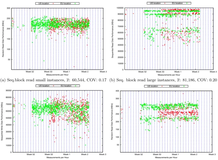
5.3 Sequential and Random I/O

We measure disk IO from three points of view: sequen-tial reads, sequensequen-tial writes, and random reads. However, since the results for sequential writes and reads are almost the same, we only present sequential read results in Fig-ure 3. We can see that the COVs of all these results are much higher than the baseline. For instance, Figure 3(a) shows the results for sequential reads on small instances. We observe that the measurements are spread over a wide

(6)

50 100 150 200 250 300

Random Read Disk Performance [KB/s]

(a) Seq.block read small instances,x: 60,544, COV: 0.17

0 10000 20000 30000 40000 50000 60000 70000 80000 90000 100000

Sequential Read Disk Performance [KB/s]

(b) Seq. block read large instances,x: 81,186, COV: 0.20

0 10000 20000 30000 40000 50000 60000 70000 80000 90000

Sequential Write Disk Performance [KB/s]

(c) Random read small instances,x: 219, COV: 0.09

50 100 150 200 250 300 350 400

Random Read Disk Performance [KB/s]

(d) Random read large instances,x: 267, COV: 0.13

Figure 3: EC2: Disk IO results for sequential and random

range, i.e. a band from approximately 55,000 to 75,000. The COV is 17%, which is much higher than baseline results (see Table 1). Figure 3 shows an interesting pattern: the mea-surements for random I/O on large instances differ consider-ably from the ones obtained in the EU. One explanation for this might be different types of disk used in different data centers. Overall we observe COVs from 9% to 20%. In con-trast, on our physical cluster we observe COVs from 0.6% to 1.9% only. So again, the difference in COV is about one order of magnitude. We expect these high COVs to have a non-negligible effect when measuring applications perform-ing large amounts of I/O-operations, e.g. MapReduce.

5.4 Network Bandwidth

The results for network performance are displayed in Fig-ure 4. The results show that instances in US location have slightly more oscillation in performance than in EU location. The COV for both instances is about 19% which is two or-ders of magnitude larger than the physical cluster having a COV of 0.2%. As for startup times, the performance varia-tion of instances in US locavaria-tion is more accented than that of instances in EU location. In theory, this could be because EC2 in the EU is relatively new and the US location is more demanded by users. As a result, more applications could be running on US location than on EU location and hence more instances share the network. However, we do not have inter-nal information from Amazon to verify this theory. Again,

0 100 200 300 400 500 600 700 800 900

Network Performance [KB/s]

Figure 4: EC2: Network perf.,x=640, COV: 0.19

we observe that the range of measurements is much bigger than for the baseline (Table 1): while the range is 6 KB/s in our physical cluster, it is 728 KB/s on EC2.

5.5 S3 Upload Speed

As many applications (such as MapReduce applications) usually upload their required data to S3, we measure the upload time to S3. We show these results in Figure 5. The mean upload time isx=120 with a COV of 54%. As men-tioned above the COV may be influenced by other traffic on

(7)

20 40 60 80 100 120 Frequency

Disk Random Read Performance (div 10000)

(a) US small instance random I/O.

10 20 30 40 50 60 70 Frequency

Disk Random Read Performance (div 10000)

(b) US large instance random I/O.

10 20 30 40 50 60 30 40 50 60 70 80 90 100 Frequency

Disk Sequential Block Read Performance (div 1000)

(c) US large instance sequential I/O perf.

10 20 30 40 50 60 Frequency

UBench CPU Performance (div 1000)

(d) US large instance Ubench CPU perf.

20 40 60 80 100 120 140 Frequency

UBench CPU Performance (div 10000)

(e) EU large instance Ubench CPU perf.

5 10 15 20 25 30 35 40 45 50 0 10 20 30 40 50 60 70 80 90 Frequency

iperf Network Performance (div 10)

(f) US network performance.

Figure 6: Distribution of measurements for different benchmarks

0 100 200 300 400 500 600

Upload Time [seconds]

Figure 5: EC2: S3 upload time, x=120, COV: 0.54

the network not pertaining to Amazon. Therefore we only show this experiment for completeness. Observe that during weeks 53 and 1 there is no data point for EU location. This is because Amazon EC2 threw us a bucket2 _{exception due}

to a naming conflict, which we fixed later on.

6. ANALYZING VARIABILITY

We observed in previous section that, in general, Amazon EC2 suffers a lot from a high variance in its performance. In the following, we analyse this in more detail. In addition, Appendix A contains a variability decomposition analysis.

6.1 Distribution Analysis

Bands. A number of previous results (e.g. Figure 2(a))

showed two performance bands in which measurements are

2_{Generally speaking, a bucket is a directory on the Cloud.}

Cutoff percent of measurements in

Lower Segment

CPU Large 320,000 22

Small 75,000 17

Memory Large 250,000 27

Small 65,000 36

Table 2: EC2: Distribution of measurements be-tween two bands for Ubench benchmark

clustered. In this section we quantify the size of some of those bands. Table 2 shows how measurements are clustered when dividing the domain of benchmark results into two partitions: one above and one below a cutoff line. The Cut-offcolumn expresses the Ubench unit that delimits the two bands and theLower Segmentcolumn presents the percent of measurements that fall into the lower segment. We can see that for CPU on large instances 22% of all measure-ments instances fall into the lower band having only 50% the performance of the upper band. In fact, several Ama-zon EC2 users already experienced this problem [3]. For me-mory performance we may observe a similar effect: 27% of the measurements are in the lower band on large instances, 36% on small instances. Thus, the lower band represents a considerable portion of the measurements.

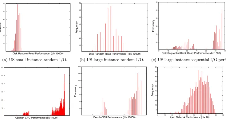
Distributions. To analyze this in more detail, we also

study the distribution of measurements of the different benchmarks. We show some representative distributions in Figure 6. We observe that measurements for Fig-ures 6(a)& 6(b), US random I/O, and Figure 6(f), US net-work performance, are normally distributed. All other dis-tributions show two bands. Most of these bands do not fol-low a normal distribution. For instance, Figure 6(c) depicts sequential I/O for large US instances. We see two bands: one very wide band spanning almost the entire domain from

(8)

0 20000 40000 60000 80000 100000 120000 140000

Instance 1 Instance 2 Instance 3 Instance 4 Instance 5

CPU performance [Ubench Score]

Instances

Xeon Opteron

Figure 7: Variability of CPU perf. per processor.

45,000 to 70,000 KB/s. In addition, we see a narrow band from 87,000 to 97,000 KB/s. None of the individual bands seems to follow a normal distribution. A possible explana-tion for this distribuexplana-tion might be cache effects, e.g. warm versus cold cache. However, a further analysis of our data could not confirm this. We thus carry out a further analysis in the following sections.

6.2 Variability over Processor Types

As indicated in [2], the EC2 infrastructure consists of two different systems — at least of two processor types3. We conducted an additional Ubench experiment so as to analyze the impact on performance that these different system types might have. To this end, we initialized 5 instances for each type of system and ran Ubench 100 times on each instance. We illustrate the results in Figure 7. These results ex-plain surprisingly in great part the two bands of CPU per-formance we observed in Section 5.1. This is surprising because both instances are assumed to provide the same performance. Here, we observe that the Opteron sor corresponds to the lower band while the Xeon proces-sor corresponds to the higher band. The variance inside these bands is then much lower than the overall variation: a COV of 1% for Xeon and a COV of 2% for Opteron — while the COV for the combined measurements was 35%. Furthermore, we could observe during this experiment that the different bands of memory performance could also be predicted using this distinction. The corresponding COV decreased from 13% for combined measurements to 1% and 6%, respectively, for Xeon and Opteron processors. Even for disk performance we found similar evidence for two seperate bands — again depending on processors.

6.3 Network Variability for Different

Locations

As described in Section 4.4, we did not explicitly consider the availability zone as a variable for our experimental setup and hence we did not pay too much attention on it in Sec-tion 5. Amazon describes each availability zone as “distinct locations that are engineered to be insulated from failures in other availability zones” [2].

In this section we analyze the impact of using different availability zones for the network benchmark. Our hypoth-esis is that whenever the two nodes running the network

3_{This can be identified by examining the}_{/proc/cpuinfo}_file

where the processor characteristics are listed.

0 100 200 300 400 500 600 700 800 900

Equal Avail Zone NEQ Availability Zone

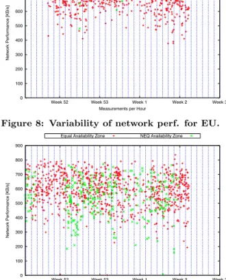
Figure 8: Variability of network perf. for EU.

0 100 200 300 400 500 600 700 800 900

Equal Availability Zone NEQ Availability Zone

Figure 9: Variability of network perf. for US.

benchmark are assigned in the same availability zone, the network performance should be better; vice versa when the two nodes are assigned to different availability zones, their network benchmark result should be worse. If this holds, we could conclude that different availability zones correspond to units (possibly physical units) where the network con-nections inside units are better than among those units.

Figure 8 shows the results for the EU. Here red indicates that both nodes run in the same availability zone, green indicates they run in different availability zones. Unfortu-nately, we observe that in the EU most instance pairs get assigned to the same availability zone. This changes however if we inspect the data for the US (see Figure 9). All mea-surements vary considerably. However, the meamea-surements inside an availability zone have a mean of 588, the measure-ments among different availability zones have a mean of 540. Thus inside an availability zone the network performance is by 9% better. We validated this result with a t-test: the null hypotheses can be rejected atp= 1.1853_×10−11_.

We believe that the variability of network performance we could observe so far might stem from the scheduler policy of EC2 — which always schedules virtual nodes of a given user to different physical nodes. This is supported by Ris-tenpart et al. who observed that a single user never gets two virtual instances running on the physical node [26]. As a consequence, this results in more network contention.

6.4 CPU Variability for Different Availability

Zones

(9)

0 100000 200000 300000 400000 500000 600000

us-east-1a us-east-1b us-east-1c us-east-1d

Figure 10: CPU distribution over different availabil-ity zones for large instances

impact CPU performance. Figure 10 shows the same data as Figure 2(b). However, in contrast to the latter, we only show data from the US and depict for each measurement its avail-ability zone. We observe that almost none of the nodes was assigned to us-east-1a or us-east-1b. All nodes were assigned to us-east-1c and to us-east-1d. Interestingly, we observe that all measurements in the second lower band belong to us-east-1c. Thus, if we ran all measurements on us-east-1d only, all measurements would be in one band. Furthermore the COV would decrease. These results confirm that indeed availability zones influence performance variation. In fact, we also observed the same influence for small instances and for other benchmarks as well, such as network performance. We believe that this is, in part, because some availability zone mainly consist of one processor type only, which in turn decreases the performance variability as discussed in Section 6.2. Hence, one should specify the availability zone when requesting its instance.

6.5 Variability over Different Instance Types

In this section, we examine the impact of different instance types on performance. Figure 11 shows the same data as Figures 2(a) and 2(b). However, in contrast to the latter we do not differentiate by location. As observed in Figure 11 the mean CPU performance of a large instance is almost exactly by a factor 4 larger than for small instances. The standard deviation for large instances is about four times higher than for small instance. However, the COVs are comparable as the factor four is removed when computing the COV. The COV is 21% for small instances and 24% for large instances. It is worth noting that the small and large instances are ac-tually based on different architectures (32/64 bit platforms, respectively), which limits the comparability between them. However, we also learn from these results is that for both instance types (small and large) several measurements may have 50% less CPU performance. instances are in the lower band? We answer this question in the next section.

6.6 Variability over Time

In previous section, we observed that, from the general point of view, most of the performance variation is indepen-dent of time. We now take a deeper look at this aspect by considering the COV for each individual weekday. Figure 12 illustrates the COV for individual weekdays for the Ubench CPU benchmark. As the COV values for other components,

0 100000 200000 300000 400000 500000 600000

Ubench CPU score

Small Instances Large Instances

Figure 11: CPU score for different instance types

0 0.05 0.1 0.15 0.2 0.25 0.3 0.35

MON TUE WED THU FRI SAT SUN

COV of Ubench CPU score

Weekday

Figure 12: Variability of CPU perf. per weekday

such as memory and network, are quite similar to those pre-sented here, we do not display those graphs. At least for the US instances we observe a lower variation in CPU per-formance of about 19% on Mondays and weekends. From Tuesday to Friday the COV is above 26%. For the EU this does not hold. The small COV for US location on Mon-day strengthen this assumption since in Unite States it is still Sunday (recall we use CET for all measurements). We believe the reason for this is that users mainly run their ap-plications during their working time. An alternative expla-nation could be that people browse and buy less on Amazon and therefore Amazon assigns more resources to EC2.

7. REAL WORLD IMPACT

So far, we ran microbenchmarks in small clusters of vir-tual nodes. Thus, natural next steps are to analyze (1) whether the performance variability observed in previous sections will average out when considering larger clusters of virtual nodes and (2) to which extent this micro variances influences actual data-intensive applications. As MapRe-duce applications are frequently performed on the Cloud, we found them to be a perfect candidate for such analysis.

7.1 Allocating Larger Clusters

For a random variable such as measurement performance one would expect that the average cluster performance will have less variance due to the larger number of ‘samples’. Therefore we experimented with different virtual cluster

(10)

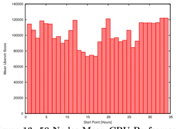
0 20000 40000 60000 80000 100000 120000 140000 0 5 10 15 20 25 30 35

Mean Ubench Score

Start Point [Hours]

Figure 13: 50 Nodes Mean CPU Performance.

sizes up to 50 nodes. However, we could not observe a sig-nificant relationship among the number of nodes and the variance. Note however, that also for the cluster 20%-30% of the measurements fall into the low performance band. Here we only show results for the largest cluster of 50 nodes we tried. As for previous experiments, we reallocated the cluster every hour. We performed this measurement for 35 hours in a row. For each hour we report the mean CPU performance of the cluster.

Figure 13 shows the results. As we may observe from the figure even when running 50 instances concurrently, the mean performance still varies considerably. Thus, a large cluster does not necessarily cancel out the variance in a way that the performance results become stable. This is because performance still depends on the number of Xeon proces-sors that composes a cluster of virtual nodes as discussed above for single virtual instances (Figure 7). It might of course be that the variance of the means will be reduced for larger clusters of several hundred nodes. Whether the means are then useful for any practical purposes or realistic applications for smaller systems as Yahoo! or Google is left to future work.

7.2 Impact on a Real Application

A natural question at this point is: How does all this variance impact performance of applications? To answer this question we use a MapReduce job as benchmark for two main reasons. First, MapReduce applications are cur-rently one of the most executed applications on the cloud and hence we believe this benchmark results would be of great interest for the community. Second, a MapReduce job usually makes intensive use of I/O (reading large datasets from disk), network (shuffling the data to reducers), CPU and main memory (parsing and sorting the data).

For this, we consider the following relation (as sug-gested in [25]), UserVisits(UV)=(sourceIP, visitedURL,

visitDate, adRevenue), which is a simplified version of a

relation containing information about the revenue generated by user visits to webpages. We use an analytic MapReduce job that computes the total sum of adRevenuegrouped by

sourceIPinUserVisitsand executed it on Hadoop 0.19.2.

We consider two variations of this job: one that runs over a dataset of 100GB and other that runs over a dataset of 25GB. We ran 3 trials for each MapReduce job every 2 hours over 50 small virtual nodes (instances). For EC2, we created a new 50-virtual nodes cluster for each series of 3 trials. In our local cluster, we executed it on 50 virtual nodes running on 10 physical nodes using Xen.

As results for the small and large MapReduce jobs follow the same pattern, we only illustrate the results for the large MapReduce job. We showed in fact these results in Figure 1 as motivation in the introduction. We observe that MapRe-duce applications suffer from much more performance vari-ability on EC2 than in our cluster. More interesting, we could again observe during these experiments that both MapReduce jobs perform better on EC2 when using larger percentage of Xeon-based systems than Opteron-based sys-tems. For example, when using more than 80% Xeon-based systems the runtime for the large MapReduce job is 840 sec-onds on average; when using less than 20% Xeon-based sys-tems the runtime is 1,100 seconds on average. This amounts to an overall COV of 11%, which might significantly impact experiments repeatability. However, even if we consider a single system type, performance variability is by an order of magnitude higher than on our local cluster.

8. LESSONS LEARNED: HINTS ON

RE-DUCING VARIABILITY

A major lesson learned from this paper is that, to run meaningful runtime experiments on EC2, users should be aware of the different physical system types4. Unfortunately, it is currently not possible to specify the processors type us-ing the EC2 API. Instead, users could report the percentage of different processors types together with their results. This would not only allow them to better predict the performance of their applications, but also to repeat their experiments. Furthermore, as re-allocating the cluster might change the system type ratio, users should use equivalent virtual cluster when comparing two applications.

We also experienced that certain availabilities zones (e.g. us-east-1d) suffer from much less performance variability as it seems they have a different ratio of processor types. Thus, users should specify one availability zone and not let the choice up to the scheduler if predictability or repeatability is crucial for their applications.

We observed that performance variability is quite high and makes it difficult to run meaningful experiments for researchers and to guarantee performance-based SLAs for companies. Thus, it is important that cloud providers of-fer performance-based SLAs guarantees to users. Further-more, given the difference in performance between Xeon and Opteron processors, we believe that EC2 should allow users to request virtual nodes using a particular underlying physical hardware confguration (CPU, memory speed, disk, network locality). For example, it seems rackspace uses so far a single processor type (Quad-Core AMD Opteron(tm) 2374 HE) only. We observed in an additional experiment on rackspace a COV of 2% for Ubench CPU performance. This is comparable to EC2 variance when only considering a single processor type. Again, it is still by an order of magnitude higher than on a local cluster.

9. CONCLUSION

This paper has provided an extensive study on the vari-ance of the current most popular Cloud computing provider Amazon EC2. We showed that performance variance on the cloud impacts a concrete MapReduce application on a 50-node cluster. We benchmarked performance micro measures

4_{Here, identified by processors type, but also having}

(11)

each hour for over one month. Our analysis clearly shows that both small and large instances suffer from a large vari-ance in performvari-ance: a COV of 24% for CPU performvari-ance; a COV of 20% for I/O performance; a COV of 19% for network performance. We could observe that one of the rea-sons of such variability is the different system types used by virtual nodes, e.g. Xeon-based systems have better per-formance than Opteron-based systems. We compared the variance on the cloud with the variance on a physical clus-ter: the results show that the MapReduce job suffered from a significantly higher performance variance on EC2.

We learned that naive runtime measurements on the cloud will suffer from high variance and will only be repeatable to a limited extent. Users should therefore conduct experiments on EC2 with care. For example, to reduce the impact of this problem, our experimental study suggests to consider the different systems type and report the used underlying sys-tem type together with the results. We also observed that as overall variance is high and measurements are not normally distributed, it may also be difficult to define meaningful, i.e. narrow, confidence intervals for measurements. However, for measurements trying to answer whether a System A is considerably better than System B, EC2 may already be used to a certain extent as explained in [18].

The performance study we presented in this paper shows many interesting avenues for further research. First, it would be interesting to discuss our results with Amazon and think about ways to reduce the variance and provide tighter SLAs. In particular, it is important to analyze how cloud providers could offer virtual nodes (instances) that allow researchers and companies to run meaningful performance experiments. Second, it would be interesting to further in-vestigate whether other cloud providers suffer from the same variance. Also, there might be even more system types. We leave this study to future work. Third, we believe that future applications can be madevariance-aware. This de-mands new techniques and algorithms which, however, goes beyond an experiments and analysis study.

10. REFERENCES

[1] 3tera, http://www.3tera.com.

[2] Amazon AWS, http://aws.amazon.com. [3] Amazon Forum, http://developer.amazonwebservices.com/connect/ thread.jspa?threadid=16912. [4] Bonnie, http://www.textuality.com/bonnie/intro.html. [5] CloudClimate, http://www.cloudclimate.com. [6] CloudKick, https://www.cloudkick.com. [7] CloudWatch, http://aws.amazon.com/cloudwatch. [8] Iperf, http://iperf.sourceforge.net/. [9] MRCloud, http://infosys.cs.uni-saarland.de/MRCloud.php. [10] Rackspace, http://www.rackspacecloud.com. [11] Ubench, http://phystech.com/download/ubench.html. [12] M. Armbrust et al. Above the Clouds: A Berkeley View of

Cloud Computing.EECS Department, UCB, Tech. Rep.

UCB/EECS-2009-28, 2009.

[13] C. Binnig, D. Kossmann, T. Kraska, and S. Loesing. How is the Weather Tomorrow?: Towards a Benchmark for the

Cloud. InTestDB Workshop, 2009.

[14] J.-D. Cryans, A. April, and A. Abran. Criteria to Compare Cloud Computing with Current Database Technology. In Conf. on Software Process and Product Measurement, 2008. [15] J. Dean and S. Ghemawat. Mapreduce: Simplified Data

Processing on Large Clusters. InOSDI, 2004.

[16] J. Dejun, G. Pierre, and C.-H. Chi. EC2 Performance Analysis for Resource Provisioning of Service-Oriented

Applications. InNFPSLAM-SOC, Nov. 2009.

[17] S. Garfinkel. An Evaluation of Amazon’s Grid Computing Services: EC2, S3 and SQS. Technical Report TR-08-07, Harvard University, July 2007.

[18] R. Jain.The Art of Computer Systems Performance

Analysis: Techniques for Experimental Design, Measurement, Simulation, and Modeling. Wiley-Interscience, 1991.

[19] K. Keahey et al. Science Clouds: Early Experiences in

Cloud Computing for Scientific Applications. InCloud

Computing and Applications, 2008.

[20] D. Kossmann, T. Kraska, and S. Loesing. An Evaluation of Alternative Architectures for Transaction Processing in the

Cloud. InSIGMOD, 2010.

[21] A. Lenk et al. What’s Inside the Cloud? An Architectural

Map of the Cloud Landscape. In ICSE Workshop on

Software Engineering Challenges of Cloud Computing, 2009.

[22] J. Li et al. Performance Model Driven QoS Guarantees and

Optimization in Clouds. InICSE CLOUD Workshop, 2009.

[23] J. Napper and P. Bientinesi. Can Cloud Computing Reach

the Top500? InWorkshops on UnConventional High

Performance Computing, 2009.

[24] S. Ostermann, A. Iosup, N. Yigitbasi, R. Prodan, T. Fahringer, and D. Epema. A Performance Analysis of EC2 Cloud Computing Services for Scientific Computing. InCloudcomp, 2009.

[25] A. Pavlo, E. Paulson, A. Rasin, D. J. Abadi, D. J. DeWitt, S. Madden, and M. Stonebraker. A Comparison of

Approaches to Large-Scale Data Analysis. InSIGMOD,

2009.

[26] T. Ristenpart et al. Hey, You, Get Off my Cloud: Exploring Information Leakage in Third-Party Compute

Clouds. InCCS Conference, 2009.

APPENDIX

A. VARIABILITY DECOMPOSITION

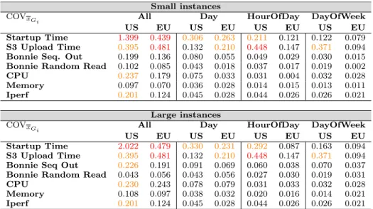
We have seen so far that Amazon EC2 suffers from a high variation in its performance. In this appendix, we decom-pose the performance variability in order to better under-stand such a variation in performance. For this, we de-compose the COV analysis into two parts with the aim of identifying from where the variance arises. To this end, we analyze the data using four different aggregation-levels: (i) day, (ii) hour, (iii) hour of the day, (iv) day of the week. We partition our measurementsx1, .., xNinto disjoint and

com-plete groupsG1, .., Gk,k≤Nwhere each group corresponds

to an aggregate of an aggregation level (i)–(iv). Then, we analyze the aggregates in two ways:

(1.) between aggregation-levels. We compute the mean

for each aggregate; then we compute the COV of all means. In other words, for each groupGiwe compute its meanxGi.

For all meansxGi we then compute the COVx_Gi. The idea

of this analysis is to show the amount of variation among

different aggregation-levels. For instance, we may answer questions like ‘does the mean change from day to day?’ Ta-ble 3 shows the results.

(2.) in aggregation-levels. We compute the COV for

each aggregate; then we compute the mean of all COVs. In other words, for each groupGi we compute its COVGi.

For all COVGiwe then compute the meanxCOV_Gi. The idea

is to show the mean variation inside different aggregation-levels. For instance, we may answer questions like ‘what is the mean variance within a day?’ Table 4 shows the results.

(12)

Small instances

COVx_Gi All Day HourOfDay DayOfWeek

US EU US EU US EU US EU

Startup Time 1.399 0.439 0.306 0.263 0.211 0.121 0.122 0.079

S3 Upload Time 0.395 0.481 0.132 0.210 0.448 0.147 0.371 0.094

Bonnie Seq. Out 0.199 0.136 0.080 0.055 0.049 0.029 0.030 0.015

Bonnie Random Read 0.102 0.085 0.043 0.018 0.037 0.017 0.019 0.002

CPU 0.237 0.179 0.075 0.033 0.031 0.004 0.032 0.028

Memory 0.097 0.070 0.036 0.028 0.014 0.015 0.013 0.011

Iperf 0.201 0.124 0.045 0.028 0.044 0.026 0.026 0.021

Large instances

COVx_Gi All Day HourOfDay DayOfWeek

Startup Time 2.022 0.479 0.330 0.231 0.292 0.087 0.163 0.094

S3 Upload Time 0.395 0.481 0.132 0.210 0.448 0.147 0.371 0.094

Bonnie Seq Out 0.226 0.191 0.091 0.069 0.060 0.038 0.070 0.037

CPU 0.230 0.243 0.078 0.079 0.031 0.033 0.032 0.028

Memory 0.108 0.097 0.038 0.032 0.020 0.016 0.014 0.021

Iperf 0.201 0.124 0.045 0.028 0.044 0.026 0.026 0.021

Table 3: between aggregation-level analysis: COV of mean values Small instances

xCOV_Gi All Day HourOfDay DayOfWeek

Startup Time 1.399 0.439 0.468 0.357 0.636 0.429 0.914 0.436

S3 Upload Time 0.395 0.481 0.356 0.406 0.371 0.448 0.383 0.472

Bonnie Seq Out 0.199 0.136 0.177 0.123 0.199 0.132 0.198 0.135

CPU 0.237 0.179 0.207 0.162 0.229 0.173 0.228 0.174

Memory 0.097 0.070 0.085 0.050 0.096 0.065 0.097 0.068

Iperf 0.201 0.124 0.204 0.121 0.196 0.122 0.205 0.123

Large instances

xCOV_Gi All Day HourOfDay DayOfWeek

Startup Time 2.022 0.479 0.330 0.330 0.812 0.416 1.192 0.451

S3 Upload Time 0.395 0.481 0.356 0.406 0.371 0.448 0.383 0.472

Bonnie Seq Out 0.226 0.191 0.227 0.183 0.227 0.192 0.317 0.189

CPU 0.237 0.243 0.208 0.222 0.235 0.242 0.236 0.242

Memory 0.108 0.097 0.093 0.085 0.105 0.096 0.107 0.095

Iperf 0.201 0.124 0.204 0.121 0.196 0.122 0.205 0.123

Table 4: in aggregation-level analysis: Mean of COV values

For better readability, all results in-between 0.2 and 0.4 are shown in orange text color, and all results greater equal 0.4 are shown in red text color.

We first discuss results in Table 3 focussing on some of the numbers marked red and orange. The results for small and large instances are very similar. Therefore we focus on discussing small instances. For small instances we observe that the mean startup time varies considerably for both US and EU: respectively 139% and 43.9% of the mean value. When aggregating by HourOfDay S3 upload times vary by 44.8% in the US but only 14.7% in the EU. When aggregat-ing by DayOfWeek we observe that mean S3 upload times also vary by 37.1% in the US but only by 9.4% in the EU. Thus, the weekday to weekday performance is more stable in the EU. CPU performance for a particular hour of the day is much more stable: 3.1% in the US and 0.4% in the EU. In addition, CPU performance for a particular day of the week is also remarkably stable: 3.2% in the US and 2.8% in the EU. We conclude that means for different hours of the day, and different days of the week show little variation. Thus a particular hour of the day or day of the week does not influence the mean performance value. Table 4 shows

results of the in-aggregation-level analysis. Here the results for small and large instances differ more widely. We focus again on small instances. For Startup Time we observe that the mean COV for Day is 46.8% in the US and 35.7% in the EU. If we aggregate by HourOfDay or DayOfWeek, we observe very high means of the COVs for both locations, e.g. up to 91.4% for DayOfWeek in the US. Thus, the mean variance for hours of the day and days of the week is very high. Still, the results in Table 3 show that the variance

among the means of a particular hour of the day or day of the week is far less. For CPU performance we observe that in the US the mean COV is above 20% when aggre-gating by Day, HourOfDay, or DayOfWeek. In other words, CPU performance varies considerablyinside each aggregate over all aggregation-levels. The variation among different aggregation-levels is not that high anymore as observed in Table 3. This indicates a certain stability of the results: the measurements inside a single aggregate may be enough to predict the mean CPU performance with little error. How-ever, recall that for our data each aggregate consists of sev-eral individual measurements: Day: 84, HourOfDay: 62, and DayOfWeek: 96 measurements.