SpatialHadoop: A MapReduce Framework for Spatial Data

SpatialHadoop: A MapReduce Framework

for Spatial Data

∗

Ahmed Eldawy

Mohamed F. Mokbel

Computer Science and Engineering, University of Minnesota, Minneapolis, MN, USA

[email protected] [email protected]

Abstract—This paper describes SpatialHadoop; a full-fledged MapReduce framework with native support for spatial data. SpatialHadoop is a comprehensive extension to Hadoop that injects spatial data awareness in each Hadoop layer, namely, the language, storage, MapReduce, andoperationslayers. In the

language layer, SpatialHadoop adds a simple and expressive high level language for spatial data types and operations. In thestoragelayer, SpatialHadoop adapts traditional spatial index structures, Grid, R-tree and R+-tree, to form a two-level spatial

index. SpatialHadoop enriches theMapReducelayer by two new

components,SpatialFileSplitterandSpatialRecordReader, for

effi-cient and scalable spatial data processing. In theoperationslayer,

SpatialHadoop is already equipped with a dozen of operations,

including range query, kNN, and spatial join. Other spatial

operations are also implemented following a similar approach. Extensive experiments on real system prototype and real datasets show that SpatialHadoop achieves orders of magnitude better performance than Hadoop for spatial data processing.

I. INTRODUCTION

Since its release in 2007, Hadoop was adopted as a solution for scalable processing of huge datasets in many applica-tions, e.g., machine learning [1], graph processing [2], and behavioral simulations [3]. Hadoop employs MapReduce [4], a simplified programming paradigm for distributed processing, to build an efficient large-scale data processing framework. The abstraction of the MapReduce programming simplifies the programming for developers, while the MapReduce framework handles parallelism, fault tolerance, and other low level issues. In the meantime, there is a recent explosion in the amounts of spatial data produced by various devices such as smart phones, satellites, and medical devices. For example, NASA satellite data archives exceeded 500 TB and is still growing [5]. As a result, researchers and practitioners worldwide have started to take advantage of the MapReduce environment in supporting large-scale spatial data. Most notably, in industry, ESRI has released ‘GIS Tools on Hadoop’ [6] that work with their flagship ArcGIS product. Meanwhile, in academia, three system prototypes were proposed: (1) Parallel-Secondo [7] as a parallel spatial DBMS that uses Hadoop as a distributed task scheduler, (2)_MD-HBase [8] extends HBase [9], a non-relational database for Hadoop, to support multidimensional indexes, and (3) Hadoop-GIS [10] extends Hive [11], a data warehouse infrastructure built on top of Hadoop with a uni-form grid index for range queries and self-join.

∗_{This work is supported in part by the National Science Foundation, USA,}

under Grants IIS-0952977 and IIS-1218168.

A main drawback in all these systems is that they still deal with Hadoop as a black box, and hence they remain limited by the limitations of existing Hadoop systems. For example, Hadoop-GIS [10], while the most advanced system prototype so far, suffer from the following limitations: (1) Hadoop itself is ill equipped in supporting spatial data as it deals with spatial data in the same way as non-spatial data. Relying on Hadoop as a black box inherits the same limitations and performance bottlenecks of Hadoop. Furthermore, Hadoop-GIS adapts Hive [11], a layer on top of Hadoop, which gives an extra overhead layer over Hadoop itself, (2) Hadoop-GIS can only support uniform grid index, which is applicable only in the rare case of uniform data distribution. (3) Being on-top of Hadoop, MapReduce programs defined through

map andreduce cannot access the constructed spatial index.

Hence, users cannot define new spatial operations beyond the already supported ones, range query and self-join. Parallel Secondo [7],MD-HBase [8], and ESRI tools on Hadoop [6] suffer from similar drawbacks.

In this paper, we introduce SpatialHadoop; a full-fledged MapReduce framework with native support for spatial data; available as open-source [12]. SpatialHadoop overcomes the limitations of Hadoop-GIS and all previous approaches as: (1) SpatialHadoop is built-in Hadoop base code (around 14,000 lines of code inside Hadoop) that pushes spatial constructs and the awareness of spatial data inside the core functionality of Hadoop. This is a key point behind the power and efficiency of SpatialHadoop. (2) SpatialHadoop is able to support a set of spatial index structures including R-tree-like indexing, which is built-in Hadoop Distributed File System (HDFS). This makes SpatialHadoop unique in terms of supporting skewed data distributions in spatial data, and (3) SpatialHadoop users can interact with Hadoop directly to develop a myriad of spatial functions. For example, in this paper, we show range queries,kNN queries, and spatial join. In another work, we show a set of computational geometry techniques that can only be realized using map and reduce

functions in SpatialHadoop [13]. This is in contrast to Hadoop-GIS and other systems that cannot support such kind of flexibility, and hence they are very limited in the functions they can support. SpatialHadoop is available as open source [12] and has been already downloaded more than 75,000 times. It has been used by several research labs and industrial companies around the world.

Objects = LOAD’points’AS(id:int, x:int, y:int); Result = FILTERObjectsBY x<x2ANDx>x1

ANDy<y2ANDy>y1;

(a) Range query in Hadoop

Objects = LOAD’points’AS(id:int, Location:POINT); Result = FILTERObjectsBY

Overlaps(Location,Rectangle(x1, y1, x2, y2));

(b) Range query in SpatialHadoop Fig. 1. Range query in Hadoop vs. SpatialHadoop

query in Hadoop and SpatialHadoop, respectively. The query finds all points located within a rectangular area represented by two corner points hx1, y1_i and hx2, y2_i. The first query statement loads an input file of points, while the second statement selects records that overlap with the given range. As Hadoop does not have any spatial indexes, it has to scan the whole dataset to answer the range query, which gives a very bad performance. In particular, it takes 200 seconds on a 20-node Hadoop cluster to process a workload of 60 GB (about 70 M spatial objects). On the other side, SpatialHadoop exploits its built-in spatial indexes to run the same query in about two seconds, which is two orders of magnitude improvement over Hadoop. In addition, the Hadoop program, written in Pig Latin language [14], is less readable due to the lack of spatial data support. SpatialHadoop uses Pigeon [15] language which makes the program simpler and more expressive as it uses spatial data types (POINT and RECTANGLE) and spatial functions (Overlaps).

SpatialHadoop is composed of four main layers, namely,

language, storage, MapReduce, and operations layers, all

injected inside the code base of Hadoop. Thelanguagelayer provides Pigeon [15], a high level SQL-like language which provides OGC-compliant [16] spatial data types and operations making it easier to adopt by users. Thestoragelayer employs a two-level index structure of globalandlocal indexing. The

global index partitions data across computation nodes while

the local index organizes data inside each node. This index

layout is used to provide three spatial indexes, namely, Grid file, R-tree and R+-tree. To make these indexes accessible to MapReduce programs, SpatialHadoop introduces two new components in theMapReducelayer, namely,

SpatialFileSplit-terandSpatialRecordReader, that exploit the global and local

index structures, respectively. Finally, the operations layer encapsulates a dozen of spatial operations that take advantage of the new components in the storage and MapReduce layers. In this paper, we only show the implementation of three basic spatial operations, namely, range query,kNN, and spatial join. A real system prototype of SpatialHadoop (available as open-source at [12]) is extensively evaluated. Experiments run on real spatial datasets extracted from NASA MODIS datasets [5] with a total size of 4.6 TB and 120 Billion records. Both SpatialHadoop and Hadoop are deployed on an internal university cluster as well as an Amazon EC2 cluster. In both platforms, SpatialHadoop has orders of magnitude better performance compared to Hadoop in all tested spatial operations (range query,kNN, and spatial join).

This paper is organized as follows: Section II highlights re-lated work. Section III gives the architecture of SpatialHadoop.

Details of thelanguage,storage,MapReduce, andoperations

layers are given in Sections IV-VII. Experiments are given in Section VIII. Section IX concludes the paper.

II. RELATEDWORK

Triggered by the needs to process large-scale spatial data, there is an increasing recent interest in using Hadoop to support spatial operations. Existing work can be classified as either specific to a certain spatial operation or a system for a suite of spatial operations. SpatialHadoop belongs to the system category, yet, with many distinguished characteristics as was discussed in section I.

Specific spatial operations. Existing work in this category has mainly focused on addressing a specific spatial operation. The idea is to develop map and reduce functions for the required operation, which will be executedon-topof existing Hadoop cluster. Examples of such work include: (1) R-tree

construction [17], where an R-tree is constructed in Hadoop

by partitioning records according to their Z-values, building a separate tree for each partition, and combining those R-trees under a common root. (2)Range query[18], [19], where the input file is scanned, and each record is compared against the query range. (3)kNN query[19], [20], where a brute force approach calculates the distance to each point and selects the closestkpoints [19], while another approach partitions points using a Voronoi diagram and finds the answer in partitions close to the query point [20]. (4)All NN (ANN) query [21], where points are partitioned according to their Z-values to find the answer similar to kNN queries. (5) Reverse NN (RNN)

query [20], where input data is partitioned by a Voronoi

diagram to exploit its properties to answer RNN queries.

(6)Spatial join [19], where the partition-based spatial-merge

join [22] is ported to MapReduce. The map function partitions the data using a grid while the reduce function joins data in each grid cell. (7)kNN join [23], [24], where the purpose is to find for each point in a setR, itskNN points from setS.

Systems. Three approaches were proposed to build systems for a suite of spatial operations: (1) Hadoop-GIS [10] extends Hive [11], a data warehouse infrastructure built on top of Hadoop, to support spatial data analysis techniques. It extends Hive with uniform grid index which is used to speed up range query and self join. Yet, Hadoop-GIS does not modify anything in the underlying Hadoop system, and hence it remains limited by the limitations of existing Hadoop systems. Also, traditional MapReduce programs that access Hadoop directly cannot make any use of Hadoop-GIS, and hence its applicability is limited. (2)_MD-HBase [8] extends HBase [9], a non-relational database runs on top of Hadoop, to support multidimensional indexes which allows for efficient retrieval of points using range and kNN queries. MD-HBase shares the same drawbacks as Hadoop-GIS, where the underlying Hadoop system remains intact, and traditional MapReduce programs will not benefit from it. (3) Parallel-Secondo [7] is a parallel spatial DBMS that uses Hadoop as a distributed task scheduler, while storage and query processing are done by spatial DBMS instances running on cluster nodes. This is

Storage MapReduce Operations

SpatialHadoop

Grid File, R-tree R+-tree Indexes SpatialRecordReader SpatialFileSplitter RangeQuery, kNN, SpatialJoin File Data System Parameters

Fig. 2. SpatialHadoop system architecture

closer in architecture and performance to parallel DBMS than Hadoop environments.

III. SPATIALHADOOPARCHITECTURE

Fig. 2 gives the high level architecture of SpatialHadoop. Similar to Hadoop, a SpatialHadoop cluster contains one master node that breaks a map-reduce job into smaller tasks, carried out by slave nodes. Three types of users interact with SpatialHadoop: (1) Casual users who access SpatialHadoop through a spatial language to process their datasets. (2)

De-velopers, who have deeper understanding of the system and

can implement new spatial operations, and (3)Administrators, who can tune up the system by adjusting system parameters in the configuration files. SpatialHadoop adopts a layered design of four main layers as described below:

(1) The language layer(Section IV) provides Pigeon [15] a simple high level SQL-like language that supports OGC-compliant spatial data types (e.g., Point and Polygon) and spatial operations (e.g., Overlap and Touches) to simplify spatial data processing. (2) In thestorage layer(Section V), SpatialHadoop employs a two-level index structure of global

and local indexing. The global index partitions data across

computation nodes while the local indexes organize data inside each node. SpatialHadoop uses the proposed structure to implement three standard indexes, namely, Grid file, R-tree and R+-R-tree. (3) SpatialHadoop adds two new components to the MapReduce layer (Section VI) to allow MapReduce programs to access the spatial index structures. The

Spatial-FileSplitterexploits the global index to prune file blocks that

do not contribute to answer, while the SpatialRecordReader

exploits local indexes to efficiently retrieve a partial answer from each block. (4) The operations layer (Section VII) encapsulates the implementation of various spatial operations that take advantage of the spatial indexes and the new com-ponents in the MapReduce layer. This paper describes the details of three of them, namely, range query,kNN, and spatial join. In another work, we implemented five computational geometry operations efficiently in SpatialHadoop [13]. More

spatial operations can be added to the operations layer using a similar approach of implementing of basic spatial operations.

IV. LANGUAGELAYER

As map-reduce-like paradigms require huge coding ef-forts [14], [25], a set of declarative SQL-like languages have been proposed, e.g., HiveQL [11], Pig Latin [14], SCOPE [25], and YSmart [26]. SpatialHadoop does not provide a com-pletely new language. Instead, it provides an extension to Pig Latin language [14], called Pigeon [15], which adds spatial data types, functions, and operations that conform to the Open Geospatial Consortium (OGC) standard [16]. In particular, we add the following:

1. Data types. Pigeon overrides the bytearray data type

to support standard spatial data types, such as, Point, LineString, and Polygon. The following code snippet loads the ‘lakes’ file with a column of typepolygon. lakes = LOAD ’lakes’ AS (id:int, area:polygon);

2. Spatial functions. Pigeon utilizes user-defined functions (UDFs) to provide spatial functions including aggregate func-tions (e.g.,Union), predicates (e.g.,Overlaps), and others (e.g., Buffer). The following code snippet shows how to use theDistancefunction to get the distance between each house and a service center with locationsc_loc.

houses_with_distance = FOREACH houses GENERATE id, Distance(house_loc, sc_loc);

3. kNN query.We enrich Pig Latin by a newKNNstatement to supportkNN queries to a given point. For example: nearest_houses = KNN houses WITH_K=100

USING Distance(house_loc, query_loc);

In addition, we override the functionality of the following two Pig Latin statements:

1. FILTER. To support a range query, we override the Pig Latin FILTER statement to accept a spatial predicate and call the corresponding procedure for range queries. Here is an example of a range query:

houses_in_range = FILTER houses BY Overlaps(house_loc, query_range);

2. JOIN. To support spatial joins, we override the Pig

LatinJOIN statement to take two spatial files as input. The processing of the JOIN statement is then forwarded to the corresponding spatial join procedure. Here is an example of a spatial join of lakes overlapping states:

lakes_states = JOIN lakes BY lakes_boundary states BY states_boundary PREDICATE = Overlaps

V. STORAGELAYER: INDEXING

Since input files in Hadoop are non-indexed heap files, the performance is limited as the input has to be scanned. To overcome this limitation, SpatialHadoop employs spatial index structures within Hadoop Distributed File System (HDFS) as a means of efficient retrieval of spatial data. Indexing in SpatialHadoop is the key point in its superior performance over Hadoop.

Traditional spatial indexes, e.g., Grid file and R-tree, are not directly applicable in Hadoop due to two challenges:

Global Index

Master Node Slave Nodes

Local Indexes

Fig. 3. Spatial indexing in SpatialHadoop

(1) Index structures are optimized for procedural program-ming, where the program executes sequential statements, while SpatialHadoop employs functional (MapReduce) pro-gramming, where the program is composed ofmapandreduce

functions executed by slave nodes. The parallel algorithms for R-trees [27] are still procedural where developers control execution of multiple threads. (2) A file in HDFS can be only written sequentially while traditional indexes are constructed incrementally. The bulk loading techniques for Grid file [28] and R-tree [29], [30] are still not applicable to the large datasets used in SpatialHadoop as they require the whole dataset to fit in memory.

As a result, existing techniques for spatial indexing in Hadoop fall in three broad categories: (1) Build only: A MapReduce approach is proposed to construct an R-tree [17], [31] but the R-tree has to be queried outside MapReduce using traditional techniques. (2) Custom on-the-fly indexing: With each query execution, a non-standard index is created and discarded after query completion, e.g., a Voronoi-based index forkNN queries [20], [23] and space-filling-curve-based indexes for range queries [21], [24]. (3) Indexing in HDFS: Up to our knowledge, only [18] builds an HDFS-based index structure for a set of trajectories. Yet, the index structure can only support range queries on trajectory data, which is a very limited functionality for what we need in SpatialHadoop.

Spatial indexing in SpatialHadoop falls under the third category as it is built inside HDFS. Yet, unlike all existing approaches, indexing in SpatialHadoop adapts HDFS to ac-commodate general purpose standard spatial index structures, namely, Grid file [32], R-tree [33] and R+-tree [34], and use them to support many spatial queries written in MapReduce. In the rest of this section, we give an overview of spatial indexing in SpatialHadoop (Section V-A). Then, we describe a generic method for building any spatial index in SpatialHadoop (Sec-tion V-B). Then, we show how the generic method is applied to build, Grid File, R-tree and R+-tree in Sections V-C to V-E.

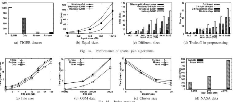
A. Overview of Indexing in SpatialHadoop

To overcome the challenges of building index structures in Hadoop, we employ a two-layers indexing approach ofglobal

andlocalindexes as shown in Fig. 3. Each index contains one

global index, stored in the Master node, that partitions data

across a set of partitions, stored in slave nodes. Each partition has a local index that organizes its own data. Such organization overcomes the above two challenges because: (1) It lends itself to MapReduce programming, where the local indexes can be processed in parallel in a MapReduce job, and (2) The small

size of local indexes allows each one to be bulk loaded in memory and written to a file in an append-only manner. The following SpatialHadoop shell command can be executed by users to index an input file src fileusing anindex-type and generate an output file dst file, where the index type can be either grid,rtree, or r+tree:

index <src file> <dst file> sindex:<index-type>

B. Index Building

Regardless of the underlying spatial index structure, an index building in SpatialHadoop is composed of three main phases, namely, partitioning, local indexing, and global

in-dexing. Details of each phase may depend on the type of the

spatial index.

1) Phase I: Partitioning: This phase spatially partitions

the input file into n partitions that satisfy three main goals:

(1) Block fit; each partition should fit in one HDFS block

of size 64 MB, (2) Spatial locality; spatially nearby objects are assigned to the same partition, and (3) Load balancing; all partitions should be roughly of the same size. To achieve these goals, we go through the following three steps:

Step 1: Number of partitions.Regardless of the spatial index type, we compute the number of partitions,n, per the equation

n=

l_S(1+α) B

m

, whereSis the input files size,Bis the HDFS block capacity (64 MB), and α is an overhead ratio, set to 0.2 by default, which accounts for the overhead of replicating records and storing local indexes. Overall, this equation adjust the average partition size to be less thanB.

Step 2: Partitions boundaries.In this step we decide on the spatial area covered by each single partition defined by a rect-angle. To accommodate data with even or skewed distribution, partition boundaries are calculated differently according to the underlying index being constructed. The output of this step is a set ofnrectangles representing boundaries of thenpartitions, which collectively cover the whole space domain.

Step 3: Physical partitioning. Given the partition bound-aries computed in Step 2, we initiate a MapReduce job that physically partitions the input file. The challenge here is to decide what to do with objects with spatial extents (e.g., polygons) that may overlap more than one partition. Some index structures assign a record to thebestmatching partition, while others replicate a record to all overlapping partitions. Replicated records are handled later by the query processor to ensure a correct answer. At the end, for each recordrassigned to a partitionp, themap function writes an intermediate pair

hp, ri. Such pairs are then grouped bypand sent to thereduce

function for the next phase, i.e.,local indexing phase.

2) Phase II: Local Indexing: The purpose of this phase is

to build the requested index structure (e.g., Grid or R-tree) as

alocal index on the data contents of each physical partition.

This is realized as a reduce function that takes the records assigned to each partition and stores them in a spatial index, written in a local index file. Each local index has to fit in one HDFS block (i.e., 64 MB) for two reasons: (1) This allows spatial operations written as MapReduce programs to access local indexes where each local index is processed in one map

(a) Grid Partitioning (b) R-tree Partitioning Fig. 4. The Partitioning Phase

task. (2) It ensures that the local index is treated by Hadoop

load balancer as one unit when it relocates blocks across

machines. According to the partitioning done in the first phase, it is expected that each partition fits in one HDFS block. In case a partition is too large to fit in one block, we break it into smaller chunks of 64 MB each, which can be written as single blocks. To ensure that local indexes remain aligned to blocks after concatenation, each file is appended with dummy data (zeros) to make it exactly 64 MB.

3) Phase III: Global Indexing: The purpose of this phase is

to build the requested index structure (e.g., Grid or R-tree) as a

globalindex that indexes all partitions. Once the MapReduce

partition job is done, we initiate an HDFSconcatcommand which concatenates all local index files into one file that represents the final indexed file. Then, the master node builds an in-memory global index which indexes all file blocks using their rectangular boundaries as the index key. The global index is constructed using bulk loading and is kept in the main memory of the master node all the time. In case the master node fails and restarts, the global index is lazily reconstructed from the rectangular boundaries of the file blocks, only when required.

C. Grid file

This section describes how the general index building algo-rithm outlined in Section V-B is used to build a grid index. The grid file [32] is a simple flat index that partitions the data according to a grid such that records overlapping each grid cell are stored in one file block as a single partition. For simplicity, we use a uniform grid assuming that data is uniformly distributed. In the partitioning phase, after the number of partitions nis calculated, partition boundaries are computed by creating a uniform grid of size ⌈√n⌉ × ⌈√n⌉

in the space domain and taking the boundaries of grid cells as partition boundaries as depicted in Fig. 4(a). This might produce more thannpartitions, but it ensures that the average partition size remains less than the HDFS block size. When physically partitioning the data, a recordrwith a spatial extent, is replicated to every grid cell it overlaps. In thelocal indexing

phase, the records of each grid cell are just written to a heap file without building any local indexes because the grid index is a one-level flat index where contents of each grid cell are stored in no particular order. Finally, the global indexing

phase concatenates all these files and builds the global index, which is a two dimensional directory table pointing to the corresponding blocks in the concatenated file.

D. R-tree

This section describes how the general index building algorithm outlined in Section V-B is used to partition spatial

data over computing nodes based on R-tree indexing, as in Fig. 4(b), followed by an R-tree local index in each partition. In the partitioning phase to compute partition boundaries, we bulk load a random sample from the input file to an in-memory R-tree using the Sort-Tile-Recursive (STR) algorithm [30]. The size of the random sample is set to a default ratio of 1% of the input file, with a maximum size of 100MB to ensure it fits in memory. Both the ratio and maximum limit can be set in configuration files. If the file contains shapes rather than points, the center point of the shape’s MBR is used in the bulk loading process. To read the sample efficiently when input file is very large, we run a MapReduce job that scans all records and outputs each one with a probability of 1%. This job also keeps track of the total size of sampled points,S, in bytes. If

S is less than 100MB, the sample is used to construct the R-tree. Otherwise, a second sample operation is executed on the output of the first one with a ratio of 100_SM B, which produces a sub-sample with an expected size of 100MB.

Once the sample is read, the master node runs the STR algorithm with the parameter d (R-tree degree) set to ⌈√n⌉

to ensure the second level of the tree contains at least n

nodes. Once the tree is constructed, we take the boundaries of the nodes in the second level and use them in the physical partitioning step. We choose the STR algorithm as it creates a balanced tree with roughly the same number of points in each leaf node. Fig. 4(b) shows an example of R-tree partitioning with 36 blocks (d= 6_{). Similar to a traditional}

R-tree, the physical partitioning step does not replicate records, but it assigns a record r to the partition that needs the least enlargement to cover r and resolves ties by selecting the partition with smallest area.

In the local indexing phase, records of each partition are bulk loaded into an R-tree using the STR algorithm [30], which is then dumped to a file. The block in a local index file is annotated with its minimum bounding rectangle (MBR) of its contents, which is calculated while building the local index. As records are overlapping, the partitions might end up being overlapped, similar to traditional R-tree nodes. The

global indexing phase concatenates all local index files and

creates the global index by bulk loading all blocks into an R-tree using their MBRs as the index key.

E. R+-tree

This section describes how the general index building al-gorithm outlined in Section V-B is used to partition spatial data over computing nodes based on tree with an R+-tree local index in each partition. R+-R+-tree [34] is a variation of the R-tree where nodes at each level are kept disjoint while records overlapping multiple nodes are replicated to each node to ensure efficient query answering. The algorithm for building an R+-tree in SpatialHadoop is very similar to that of the R-tree except for three changes. (1) In the R+-tree physical partitioning step, each record is replicated to each partition it overlaps with. (2) In thelocal indexingphase, the records of each partition are inserted into an R+-tree which is then dumped to a local index file. (3) Unlike the case of

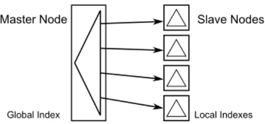
Fig. 5. R+-tree index for road segments in the whole world extracted from OpenStreetMap (Best viewed in color)

R-tree, the global index is constructed based on the partition boundaries computed in the partitioning phase rather than the MBR of its contents as boundaries should remain disjoint. These three changes ensure that the constructed index satisfies the properties of the R+-tree.

Fig. 5 gives a prime example behind the need for R+-tree (and R-tree) indexing in SpatialHadoop, which also shows the key behind SpatialHadoop performance. The figure shows the partitioning of an R+-tree index constructed on a 400 GB file that includes all the road networks (depicted in blue lines) extracted from OpenStreetMap [35]. The black rectangles in the figure indicate partition boundaries of the global index. While some road segments cross multiple partitions, partition boundaries remain disjoint due to the properties of the R+-tree. As each partition is sufficient for only 64 MB worth of data, we can see that dense areas (e.g., Europe) are contained in very small partitions, while sparse areas (e.g., oceans) are contained in very large partitions. One way to look at this figure is that this is the way that SpatialHadoop divides a dataset of 400 GB into small chunks, each of 64 MB which is the key point behind the order of magnitude performance that SpatialHadoop got over traditional Hadoop.

VI. MAPREDUCELAYER

Similar to Hadoop, the MapReduce layer in SpatialHadoop is the query processing layer that runs MapReduce programs. However, contrary to Hadoop where the input files are non-indexed heap files, SpatialHadoop supports spatially non-indexed input files. Fig. 6 depicts part of the MapReduce plan in both Hadoop and SpatialHadoop, where the modifications in SpatialHadoop are highlighted. In Hadoop (Fig. 6(a)), the input file goes through a FileSplitter that divides it into n splits, wheren is set by the the MapReduce program, based on the number of available slave nodes. Then, each split goes through

aRecordReaderthat extracts records as key-value pairs which

are passed to the map function. SpatialHadoop (Fig. 6(b)) enriches traditional Hadoop systems by two main components: (1)SpatialFileSplitter(Section VI-A); an extended splitter that exploits the global index(es) on input file(s) to early prune file blocks not contributing to answer, and (2)

SpatialRecor-Number of Splits (n) Map Split Map task Record Reader k, v ... k, v Map Split Map task Record Reader k, v_... k, v Heap File #1 #n ... n 1 File Splitter (a) Hadoop Spatial File Splitter Number of Splits (n) Spatial Record Reader Map Split Map task Local Index(es) Spatial Record Reader Map Split Map task Local Index(es) Spatially Indexed Files Filter Function #1 #n ... n 1 (b) SpatialHadoop

Fig. 6. Map phase in Hadoop and SpatialHadoop

dReader(Section VI-B), which reads a split originating from

spatially indexed input file(s) and exploits the local indexes to efficiently process it.

A. SpatialFileSplitter

Unlike the traditional file splitter, which takes one input file, the SpatialFileSplitter can take one or two input files where the blocks in each file are globally indexed. In addition,

the SpatialFileSplittertakes a filter function, provided by the

developer to filter file blocks that do not contribute to answer. A single file input represents unary operations, e.g., range andk-nearest-neighbor queries, while two input files represent binary operations, e.g., spatial join.

In case of one input file, theSpatialFileSplitterapplies the filter function on the global index of the input file to select file blocks, based on their MBRs, that should be processed by the job. For example, a range query job provides a filter function that prunes file blocks with MBRs completely outside the query range. For each selected file block in the query range, theSpatialFileSplittercreates a file split, to be processed later by theSpatialRecordReader. In case of two input files, e.g., a spatial join operation, the behavior of theSpatialFileSplitteris quite similar with two subtle differences: (1) The filter function is applied to two global indexes; each corresponds to one input file. For example, a spatial join operation selects pairs

of blocks with overlapping MBRs. (2) The output of the Spa-tialFileSplitteris a combined split that contains a pair of file ranges (i.e., file offsets and lengths) corresponding to the two selected blocks from the filter function. This combined split is passed to the SpatialRecordReaderfor further processing.

B. SpatialRecordReader

The SpatialRecordReadertakes either a split or combined

split, produced from the SpatialFileSplitter, and parses it to generate key-value pairs to be passed to the map function. If the split is produced from a single file, the

SpatialRecor-dReader parses the block to extract the local index that acts

as an access method to all records in the block. Instead of passing records to the map function one-by-one as in traditional Hadoop record readers, the record reader sends all the records to the map function indexed by the local index. This has two main benefits: (1) it allows the map function to process all records together, which is shown to make it more powerful and flexible [20], and (2) the local index is harnessed when processing the block, making it more efficient than scanning over all records. To adhere with the key-value record format, we generate a key-value pair _hmbr, lindex_i, where the key is the MBR of the assigned block and the value is a pointer to the loaded local index. The traditional record reader is still supported and can be used to iterate over records in case the local index is not needed.

In case the split is produced from two spatially indexed input files, the SpatialRecordReader parses the two blocks stored in the combined split and extracts the two local indexes in both blocks. It then builds one key-value pair

hhmbr1, mbr2_i,_hlindex1, lindex2_ii, which is sent to the map function for processing. The key is a pair of MBRs, each corresponds to one block, while the value is a pair of pointers, each points to a local index extracted from a block.

VII. OPERATIONSLAYER

The combination of the spatial indexing in the storage layer (Section V) with the new spatial functionality in the MapReduce layer (Section VI) gives the core of SpatialHadoop that enables the possibility of efficient realization of a myriad of spatial operations. In this section, we only focus on three basic spatial operations: range query (Section VII-A), kNN (Section VII-B), and spatial join (Section VII-C), as three case studies of how to use SpatialHadoop. SpatialHadoop contains also computation geometry operations [13] and more operations, e.g., kNN join, and RNN, can also be realized in SpatialHadoop following a similar approach.

A. Range Query

A range query takes a set of spatial recordsR and a query area A as input, and returns the set of records in R that overlaps with A. In Hadoop, the input set is provided as a heap file, hence, all records have to be scanned to output matching records. SpatialHadoop achieves orders of magnitude speedup by exploiting the spatial index. There are two range

query techniques implemented in SpatialHadoop depending on whether the index replicates entries or not.

No replication.In case of R-tree, where each record is stored in exactly one partition, the range query algorithm runs in two steps. (1) Theglobal filterstep, which selects file blocks that need to be processed. This step exploits the global index through feeding the SpatialFileSplitter with a range filter to select those blocks overlapping with the query areaA. Blocks that are completely inside the query area are copied to the output without any further processing as all its records are within the query range. Blocks that are partially overlapping are sent for further processing in the second step. (2) The

local filterstep operates on the granularity of a file block and exploits the local index to return records overlapping with the query area. TheSpatialRecordReaderreads a block that needs to be processed, extracts its local index, and sends it to the map function, which exploits the local index with a traditional range query algorithm to return matching records.

Replication.In case of Grid and R+-tree where some records are replicated across partitions, the range query algorithm differs from the one described above in two main points: (1) In the global filter step, blocks that are completely contained in the query area A have to be further processed as they might have duplicate records that need to be removed. (2) The output of the local filter goes through an additionalduplicate

avoidance[36] step to ensure that duplicates are removed from

the final answer. For each candidate record produced by the local filter step, we compute its intersection with the query area. A record is added to the final result only if the top-left corner of the intersection is inside the partition boundaries. Since partitions are disjoint, it is guaranteed that only one partition contains that point. The output of the duplicate avoidance step gives the final answer of the range query, hence, no reduce function is needed.

B. k Nearest Neighbor (kNN)

AkNN query takes a set of spatial pointsP, a query point

Q, and an integerk as input, and returns thekclosest points in P toQ. In Hadoop, a kNN algorithm scans all points in the input file, calculates their distances to Q, and produces the top-k ones [19]. With SpatialHadoop, we exploit simple pruning techniques that achieve orders of magnitude better performance than that of Hadoop. A kNN query algorithm in SpatialHadoop is composed of the three steps: (1) Initial

answer, where we come up with an initial answer of the k

closest points toQwithin the same file block (i.e., partition) as Q. We first locate the partition that includesQ by feeding

the SpatialFileSplitter with a filter function that selects only

the overlapping partition. Then, the selected partition goes through theSpatialRecordReaderto exploit its local index with a traditionalkNN algorithm to produce the initialk answers.

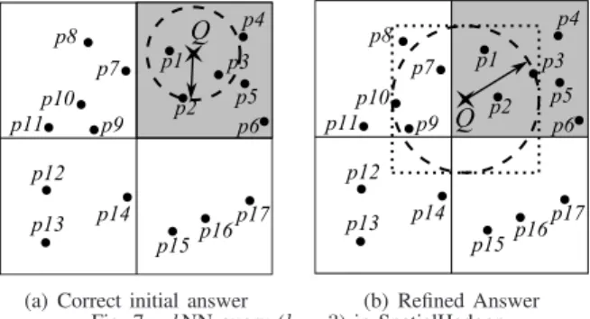
(2) Correctness check, where we check if the initial answer

can be considered final. We draw a test circle C centered at Q with a radius equal to the distance from Q to its kth furthest neighbor, obtained from the initial answer. IfC does not overlap any partition other thanQ, we terminate and the

Q p1 p2 p3 p4 p5 p6 p8 p7 p9 p10 p11 p12 p13 p14 p15 p16 p17

(a) Correct initial answer

Q p1 p2 p3 p4 p5 p6 p8 p7 p9 p10 p11 p12 p13 p14 p15p16 p17 (b) Refined Answer Fig. 7. kNN query (k= 3_{) in SpatialHadoop}

initial answer is considered final. Otherwise, we proceed to the third step. (3)Answer Refinement, where we run a range query to get all points inside the MBR of the test circleC, obtained from previous step. Then, a scan over the range query result is executed to produce the closestkpoints as the final answer. Fig. 7 gives two examples of akNN query for pointQ(in a shaded partition) withk=3. In Fig. 7a, the dotted test circleC, composed from the initial answer{p1,p2,p3}, overlaps only the shaded partition. Hence, the initial answer is considered final. In Fig. 7b, the circle C intersects other blocks. Hence, a range query is issued with the MBR of C, and a refined answer is produced as {p1,p2,p7}, wherep7 is closer toQ

thanp3.

C. Spatial Join

A spatial join takes two sets of spatial recordsRandSand a spatial join predicateθ(e.g.,overlaps) as input, and returns the set of all pairshr, siwherer∈R,s∈S, andθis true for

hr, si. In Hadoop, the SJMR algorithm [37] is proposed as the MapReduce version of the partition-based spatial-merge join (PBSM) [22]; a classic spatial join algorithm for distributed systems. SJMR employs a map function that partitions input records according to a uniform grid, and then a reduce function that joins records in each partition. Though SJMR is designed for Hadoop, it can still run, as is, on SpatialHadoop, yet with a better performance since the input files are already partitioned. To better utilize the spatial indexes, we equip SpatialHadoop with a novel spatial join algorithm, termed

distributed joinwhich is composed of three main steps, namely

global join,local join, andduplicate avoidance. In some cases, an additional preprocessing step can be added to speed up the distributed join algorithm.

Step 1: Global join. Given two input files of spatial records

R and S, this step produces all pairs of file blocks with overlapping MBRs. Apparently, only an overlapping pair of blocks can contribute to the final answer of the spatial join since records in twonon-overlappingblocks are definitely dis-joint. To produce the overlapping pairs, theSpatialFileSplitter

module is fed with the overlapping filter function to exploit two spatially indexed input files. Then, a traditional spatial join algorithm is applied over the two global indexes to produce the overlapping pairs of partitions. TheSpatialFileSplitterwill finally create a combined split for each pair of overlapping blocks.

Step 2: Local join. Given a combined split produced from the previous step, this step joins the records in the two blocks

Roads

Rivers

Overlapping Partitions

Fig. 8. Distributedjoin between roads and rivers

in this split to produce pairs of overlapping records. To do so,

theSpatialRecordReaderreads the combined split, extracts the

records and local indexes from its two blocks, and sends all of them to the map function for processing. The map function exploits the two local indexes to speed up the process of joining the two sets of records in the combined split. The result of the local join may contain duplicate results due to having records overlapping with multiple blocks.

Step 3: Duplicate avoidance. Similar to the case of range queries, this step runs only for indexes with replication (i.e., Grid and R+-tree) and employs the reference-point duplicate avoidance technique [36]. For each detected overlapping pair of records, the intersection of their MBRs is first computed. Then, the overlapping pair is reported as a final answer only if the top-left corner (i.e.,reference point) of the intersection falls in the overlap of the MBRs with the two processed blocks.

Example. Fig. 8 gives an example of a spatial join between a file ofRoadsand a file ofRivers. As both files are par-titioned using the same 4×4 grid structure, there is no need for a preprocessing step. The global join step is responsible on matching the overlapped partitions together. The local join step joins the contents of each matched partitions. Finally, the duplicate avoidance step ensures that each matched record is produced only once.

Fig. 9. Partitions.

Preprocessing step. The two input files to the spatial join could be partitioned inde-pendently upon their loading into Spatial-Hadoop. For example, Figure 9 gives an example of joining two grid files with 3

× 3 (solid lines) and 4 ×4 (dotted lines) grids. In this case, our distributed spatial

join algorithm has two options to proceed: (1) Work exactly as described above without any preprocessing, where joining the two grid files produces 36 overlapping pairs of grid cells that are processed in 36 map tasks, or (2) Repartitioning the smaller file (the one with 9 cells) into 16 partitions to match the same partitioning of the larger one. Hence, the number of overlapping pairs of grid cells is decreased from 36 to 16. There is a clear trade-off between these two options. The repartitioning step is costly, yet it reduces the time required for joining as there are less overlapping grid cells. To decide whether to run the preprocessing step or not, SpatialHadoop estimates the cost in both cases and chooses the one with least estimated cost. For simplicity, we use the number of map tasks as an estimator for the cost. When the two files are joined directly, the number of map tasks mj is the total

number of overlapping blocks in the two files. When adding the preprocessing step, the number of map tasks mp is the sum of the number of blocks in both files. This is because the preprocessing step reads and partitions every block in the smaller file, then joins with every block in the larger file. Only if mp < mj, the preprocessing step is carried out, otherwise, the files are joined directly.

VIII. EXPERIMENTS

This section provides an extensive experimental study for the performance of SpatialHadoop compared to standard Hadoop. We decided to compare with standard Hadoop and not other parallel spatial DBMSs for two reasons. First, as our contributions are all about spatial data support in Hadoop, the experiments are designed to show the effect of these additions or the overhead imposed by the new features compared to a tra-ditional Hadoop. Second, the different architectures of spatial DBMSs have great influence on their respective performance, which are out of the scope of this paper. Interested readers can refer to a previous study [38] which has been established to compare different large scale data analysis architectures. Meanwhile, we could not compare with MD-HBase [8] or Hadoop-GIS [10] as they support much limited functionality than what we have in SpatialHadoop. Also, they rely on the existence of HBase or Hive layers, respectively, which we do not currently have in SpatialHadoop. SpatialHadoop (source code is available at: [12]) is implemented inside Hadoop 1.2.1 on Java 1.6. All experiments are conducted on an Amazon EC2 [39] cluster of up to 100 nodes. The default cluster size is 20 nodes of ‘small’ instances.

Datasets. We use the following real and synthetic datasets to test various performance aspects for SpatialHadoop: (1) TIGER: A real dataset which represents spatial features in the US, such as streets and rivers [40]. It contains 70M line segments with a total size of 60 GB. (2) OSM: A real dataset extracted from OpenStreetMap [35] which represents map data from the whole world. It contains 164M polygons with a total size of 60 GB. (3) NASA: Remote sensing data which represents vegetation indices for the whole world over 14 years. It contains 120 Billion points with a total size of 4.6 TB. (4) SYNTH: A synthetic dataset generated in an area of 1M × 1M units, where each record is a rectangle of maximum sized_×d;dis set to 100 by default. The location and size of each record are both generated based on a uniform distribution. We generate up to 2 Billion rectangles of total size 128 GB. To allow researchers to repeat the experiments, we make the first two datasets available on SpatialHadoop web-site. The third dataset is already made available by NASA [5]. The generator is shipped as part of SpatialHadoop and can be used as described in its documentation.

In our experiments, we compare the performance of the range query,kNN, and distributed join algorithms in Spatial-Hadoop proposed in Section VII to their traditional imple-mentation in Hadoop [19], [37]. For range query and kNN, we use system throughput as the performance metric, which indicates the number of MapReduce jobs finished per minute.

To calculate the throughput, a batch of 20 queries is submitted to the system to ensure full utilization and the throughput is calculated by dividing 20 over the total time to answer all the queries. For spatial join, we use the processing time of one query as the performance metric as one query is usually enough to keep all machines busy. The experimental results for range queries, kNN queries, and spatial join are reported in Sections VIII-A, VIII-B, and VIII-C, respectively, while Section VIII-D studies the performance of index creation.

A. Range Query

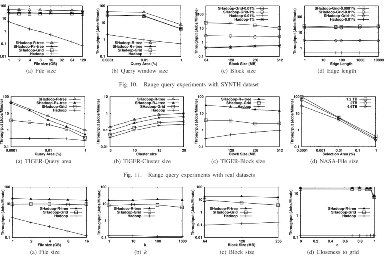
Figures 10 and 11 give the performance of range query pro-cessing on Hadoop [19] and SpatialHadoop for both SYNTH and real datasets, respectively. Queries are centered at random points sampled from the input file. The generated query workload has a natural skew where dense areas are queried with higher probability to simulate realistic workloads. Unless mentioned otherwise, we set the file size to 16 GB, query area size to 0.01% of the space, block size to 64 MB, and edge length of generated rectangles to 100 units.

In Fig. 10(a), we increase the file size from 1 GB to 128 GB, while measuring the throughput of Hadoop, Spa-tialHadoop with Grid, R-tree and R+-tree indexes. For all file sizes, SpatialHadoop has consistently one or two orders of magnitude higher throughput due to pruning employed by the SpatialFileSplitter and the global index. As Hadoop needs to scan the whole file, its throughput decreases with the increase in file size. On the other hand, the throughput of SpatialHadoop remains stable as it processes only a fixed area of the input file. As data is uniformly distributed, R+-tree becomes similar to the grid file with the addition of a local index in each block. R-tree is significantly better as it skips processing of partitions completely contained in the query range while R+-tree suffers from the overhead of replication and duplicate avoidance technique. In Fig. 10(b), the query area increases from 0.0001% to 1% of the total area. In all cases, SpatialHadoop gives more than an order of magnitude better throughput than Hadoop. The throughput of both systems decreases with the increase of the query area, where: (a) we need to process more file blocks, and (b) The size of the output file becomes larger. R-tree is more resilient to increased query areas as it skips processing of blocks totally contained in query area as well as duplicate avoidance.

Fig. 10(c) gives the effect of increasing the block size from 64 MB to 512 MB, while measuring the throughput of Hadoop and SpatialHadoop for two sizes of the query area, 1% and 0.01%. For clarity, we show only the grid index as other indexes produce similar trends. When increasing block size, Hadoop performance slightly increases as it requires less number of blocks to process while SpatialHadoop performance decreases as the number of processed blocks remain the same while block sizes increase. Fig. 10(d) gives the overhead of the duplicate avoidance technique used in grid and R+-tree indexing. The edges length of spatial data is increased from 1 to 10K within a space area of 1M×1M, which increases replication in the indexed file. As shown in figure, the overhead

0.01 0.1 1 10 100 1 2 4 8 16 32 64 128 Throughput (Jobs/Minute) File size (GB) SHadoop-R-tree SHadoop-R+-tree SHadoop-Grid Hadoop

(a) File size

0.1 1 10 100 0.0001 0.01 1 Throughput (Jobs/Minute) Query Area (%) SHadoop-R-tree SHadoop-R+-tree SHadoop-Grid Hadoop

(b) Query window size

0.1 1 10 100 64 128 256 512 Throughput (Jobs/Minute) Block Size (MB) SHadoop-Grid-0.01% SHadoop-Grid-1% Hadoop-0.01% Hadoop-1% (c) Block size 1 10 100 1 10 100 1000 10000 Throughput (Jobs/Minute) Edge Length SHadoop-Grid-0.0001% SHadoop-Grid-0.01% SHadoop-Grid-1% Hadoop-0.01% (d) Edge length Fig. 10. Range query experiments with SYNTH dataset

0.1 1 10 100 0.0001 0.01 1 Throughput (Jobs/Minute) Query Area (%) SHadoop-R-tree SHadoop-R+-tree SHadoop-Grid Hadoop

(a) TIGER-Query area

0.01 0.1 1 10 5 10 15 20 Throughput (Jobs/Minute) Cluster size SHadoop-R-tree SHadoop-R+-tree SHadoop-Grid Hadoop (b) TIGER-Cluster size 0.1 1 10 100 128 256 512 Throughput (Jobs/Minute) Block Size (MB) SHadoop-R+-tree SHadoop-Grid Hadoop (c) TIGER-Block size 0.1 1 10 100 0.0001 0.001 0.01 0.1 1 Throughput (Jobs/Minute) Selection Area (%) 1.2 TB 2TB 4.6TB (d) NASA-File size Fig. 11. Range query experiments with real datasets

0.1 1 10 100 1 2 4 8 16 Throughput (Jobs/Minute) File size (GB) SHadoop-R-tree SHadoop-Grid Hadoop

(a) File size

0.1 1 10 100 1 10 100 1000 Throughput (Jobs/Minute) k SHadoop-R-tree SHadoop-Grid Hadoop (b)k 0.01 0.1 1 10 100 64 128 256 Throughput (Jobs/Minute) Block Size (MB) SHadoop-R-tree SHadoop-Grid Hadoop (c) Block size 0.1 1 10 0 0.2 0.4 0.6 0.8 1 Throughput (Jobs/Minute) c SHadoop-R-tree SHadoop-Grid Hadoop (d) Closeness to grid Fig. 12. kNN algorithms with SYNTH dataset

of the duplicate avoidance technique ends up to be minimal and SpatialHadoop manages to keep its performance within orders of magnitude higher throughput.

Fig. 11(a) gives the performance of range query on the TIGER dataset when increasing the query area. SpatialHadoop shows two orders of magnitude throughput increase over traditional Hadoop. Unlike the SYNTH dataset where grid and R-tree indexes behave similarly, the TIGER dataset is more suited with an R-tree index due to the natural skewness in the data. Fig. 11(b) shows how SpatialHadoop scales out with cluster size changing from 5 to 20 nodes when executing range queries with a selection area of 1%. Both Hadoop and SpatialHadoop scale smoothly with cluster size, while SpatialHadoop is consistently more efficient. Fig. 11(c) shows how block size affects the performance of range queries on the TIGER real dataset. The results here conforms with those of synthetic dataset in Fig. 10(c) where Hadoop performance is enhanced while SpatialHadoop degrades a little bit. The difference here is higher due to the high skewness of the TIGER dataset. Fig. 11(d) shows the running time for range queries on subsets of NASA dataset of sizes 1.2TB, 2TB and the whole dataset of size 4.6TB. The datasets are indexed using R-tree on an EC2 cluster of 100largenodes, each with a quad core processor and 8GB of memory. This experiment shows the high scalability of SpatialHadoop in terms of data size and number of machines where it takes only a couple of minutes with the largest selection area on the 4.6TB dataset.

B. K-Nearest-Neighbor Queries (kNN)

Figures 12 and 13 give the performance ofkNN query pro-cessing on Hadoop [19] and SpatialHadoop for both SYNTH and TIGER datasets, respectively. In both experiments, query locations are set at random points sampled from the input file. Unless otherwise mentioned, we set the file size to 16 GB,k

to 1000, and block size to 64 MB. We omit the results of the R+-tree as it becomes similar to R-tree when indexing points because there is no replication.

Fig. 12(a) measures system throughput when increasing the input size from 1 GB to 16 GB. SpatialHadoop has one to two orders of magnitude higher throughput. Hadoop performance decreases dramatically as it needs to process the whole file while SpatialHadoop maintains its performance as it processes one block regardless of the file size. Unlike the case of range queries, the R-tree with local index shows a significant speedup as it allows thekNN to be calculated efficiently within each block, while the grid index has to scan each block. Ask

is varied from 1 to 1000 in Fig. 12(b), SpatialHadoop keeps its speedup at two orders of magnitude askis small compared to number of records per block.

In Fig. 12(c), as the block size increases from 64 MB to 256 MB, the performance of SpatialHadoop stays at two orders of magnitude higher than Hadoop. Since Hadoop scans the whole file, it becomes a little bit faster with larger block sizes as the number of blocks gets lower. Fig. 12(d) shows how the throughput is affected by the location of the query point Q

0.1 1 10 100 1 10 100 1000 Throughput (Jobs/Minute) k SHadoop-R-tree SHadoop-Grid Hadoop (a)k 0.1 1 10 100 64 128 256 512 Throughput (Jobs/Minute) Block Size (MB) SHadoop-R-tree SHadoop-Grid Hadoop (b) Block size Fig. 13. Performance ofkNN with TIGER dataset

relative to the boundary lines of the global index partitions. Rather than generated totally at random, the query points are placed on the diagonal of a random partition where its distance to the center of the partition is controlled by acloseness factor 0 _{≤ c ≤} 1_{; 0 means that Q is in the partition center while}

1 means that Q is a corner point. When c is close to zero, the query answer is likely to be found in one partition. When

c is close to 1, it is likely that we need to refine the initial answer, which significantly decreases throughput, yet it is still of two orders of magnitude higher than Hadoop, which is not affected by the value of c.

Fig. 13(a) gives the effect of increasing k from 1 to 1000 on TIGER dataset. While all algorithms seem to be unaffected by k as discussed earlier, SpatialHadoop gives an order of magnitude performance with grid index and two orders of magnitude performance with an R-tree index. Fig. 13(b) gives the effect of increasing the block size from 64 MB to 512 MB. While the performance with grid index tends to decrease with increased block sizes, the R-tree remains stable for higher block sizes. The performance of Hadoop increases with higher block sizes due to the decrease in total number of map tasks.

C. Spatial Join

Fig. 14 gives the results of the spatial join experiments, where we compare ourdistributedjoin algorithm for Spatial-Hadoop with two implementations of the SMJR algorithm [37] on Hadoop and SpatialHadoop. Fig. 14(a) gives the total processing time for joining edges and linearwater files from TIGER dataset of sizes 60GB and 20GB, respectively. Both R-tree and R+-tree give the best results as they deal well with skewed data with the R+-tree significantly better due to the non-overlapping partitions. Both Grid index and SJMR give poor performance as they use a uniform grid.

Fig. 14(b) gives the response time of joining two generated files of the same size (1 to 16GB). To keep the figures concise, we show only the performance of the distributed join algorithm operating on R-tree indexed files as other indexes give similar trends. In all cases, our distributed join algorithm shows a significant speedup over SJMR in Hadoop. Moreover, SJMR runs faster on SpatialHadoop compared to Hadoop as the partition step becomes more efficient when the input file is already partitioned. In Fig. 14(c), the response times of the different spatial join algorithms are depicted when the two input files are of different sizes. In this case, a preprocessing step may be needed which is indicated by a black bar. For small file sizes, the distributed join carries out the join step directly as the repartition step is costly compared to the join

step. In all cases, distributed join significantly outperforms other algorithms with double to triple performance, while SJMR on Hadoop gives the worst performance as it needs to partition both input files.

Fig. 14(d) highlights the tradeoff in the preprocessing step. We rerun the same join experiments of two different file sizes with and without a preprocessing step. We also run a third instance (DJ-Smart) that decides whether to run a preprocessing step or not based on the number of map tasks in each case as discussed in Section VII-C. DJ-Smart manages to take the right decision in most cases. It only misses the right decision in two cases where it performs the preprocessing step when the direct join is faster. Even for these two cases, the difference in processing time is very small and does not cause major degradation in performance. The figure also shows that for some cases, such as1_×8_{, the preprocessing step manages}

to speedup the join step but it incurs a big overhead rendering it to be unuseful for this case.

D. Index Creation

Fig. 15 gives the time spent for building the spatial index in SpatialHadoop. This is a one time job done when loading a file and the index can be used many times in subsequent queries. Fig. 15(a) shows a good scalability for indexing schemes when indexing a generated file with a size varying from 1 GB to 128 GB. For example, it builds an R-tree index for a 128 GB file with more than 2 Billion records in about one hour on 20 machines. The grid index is faster as it basically partitions the data using a uniform grid while the R-tree takes more time for reading the random sample from the file, bulk loading it into an R-tree and building local indexes. Fig. 15(b) shows a similar behavior when indexing real data from OpenStreetMap. Fig. 15(c) shows a near linear scale up for all indexing schemes when the cluster size increases from 5 to 20 machines.

To take SpatialHadoop to an extreme, we test it with NASA datasets of up to 4.6TB and 120 Billion records on a 100-node cluster of Amazon ‘large’ instances. Fig. 15(d) shows the indexing time for an R-tree index. As shown, it takes less than 15 hours do build a highly efficient R-tree index for a 4.6 TB dataset which renders SpatialHadoop very scalable in terms of data size and number of machines. Note that building the index is a one time process for the whole data, after which the index lives for long. The figure also shows that the time spent in reading the sample and constructing the in-memory R-tree using STR (Section V-D) is very small compared to the total time of indexing.

IX. CONCLUSION

This paper introduces SpatialHadoop, a full-fledged MapRe-duce framework with native support for spatial data available as free open-source. SpatialHadoop is a comprehensive ex-tension to Hadoop that injects spatial data awareness in each Hadoop layer, namely, the language, storage, MapReduce,

and operations layers. In the languagelayer, SpatialHadoop

0 200 400 600 800 1000 1200 Time (min) R+-tree R-tree Grid SJMR

(a) TIGER dataset

20 40 60 80 100 120 1x1 2x2 4x4 8x8 16x16 Time (min) Input sizes (GB) SHadoop-DJ SHadoop-SJMR Hadoop-SJMR (b) Equal sizes 0 20 40 60 80 100 120 140 Time (min) Input sizes (GB) SHadoop-DJ-Preprocess SHadoop-DJ-Join SHadoop-SJMR Hadoop-SJMR 8x16 4x16 2x16 1x16 1x8 1x4 1x2 (c) Different sizes 0 20 40 60 80 Time (min) Input sizes (GB) DJ-Smart DJ-Join directly DJ-Repartition step DJ-Join step 8x16 4x16 2x16 1x16 1x8 1x4 1x2 (d) Tradeoff in preprocessing Fig. 14. Performance of spatial join algorithms

5 15 50

1 2 4 8 16 32 64 128

Time (min) - Log scale

File size (GB) R-tree

R+-tree Grid

(a) File size

5 15 50

102MB 0.9GB 2.6GB 20GB

Time (min) - Log scale

File size R+-tree R-tree Grid (b) OSM data 5 15 30 5 10 15 20

Time (min) - Log scale

Cluster size R+-tree R-tree Grid (c) Cluster size 0 100 200 300 400 500 600 700 800 900 Time (min) Input sizes (TB) Sample Index 4.6TB 2TB 1.2TB (d) NASA data Fig. 15. Index creation

support for spatial data types and operations. In the storage

layer, SpatialHadoop adapts traditional spatial index struc-tures, Grid, R-tree, and R+-tree, to form a two-level spatial index for MapReduce environments. In the MapReducelayer, SpatialHadoop enriches Hadoop with two new components,

SpatialFileSplitterandSpatialRecordReader, for efficient and

scalable spatial data processing. In the operations layer, SpatialHadoop is already equipped with three basic spatial operations, range query,kNN, and spatial join, as case studies for implementing spatial operations. Other spatial operations can also be added following a similar approach. Extensive experiments, based on a real system prototype and large-scale real datasets of up to 4.6TB, show that SpatialHadoop achieves orders of magnitude higher throughput than Hadoop for range and k-nearest-neighbor queries and triple performance for spatial joins.

REFERENCES

[1] A. Ghoting, “et. al. SystemML: Declarative Machine Learning on MapReduce,” inICDE, 2011.

[2] http://giraph.apache.org/.

[3] G. Wang, M. Salles, B. Sowell, X. Wang, T. Cao, A. Demers, J. Gehrke, and W. White, “Behavioral Simulations in MapReduce,”PVLDB, 2010. [4] J. Dean and S. Ghemawat, “MapReduce: Simplified Data Processing on

Large Clusters,”Communications of ACM, vol. 51, 2008.

[5] http://aws.amazon.com/blogs/aws/process-earth-science-data-on-aws-with-nasa-nex/. [6] http://esri.github.io/gis-tools-for-hadoop/.

[7] J. Lu and R. H. Guting, “Parallel Secondo: Boosting Database Engines with Hadoop,” inICPADS, 2012.

[8] S. Nishimura, S. Das, D. Agrawal, and A. El Abbadi, “MD-HBase: Design and Implementation of an Elastic Data Infrastructure for Cloud-scale Location Services,”DAPD, vol. 31, no. 2, pp. 289–319, 2013. [9] “HBase,” 2012, http://hbase.apache.org/.

[10] A. Aji, F. Wang, H. Vo, R. Lee, Q. Liu, X. Zhang, and J. Saltz, “Hadoop-GIS: A High Performance Spatial Data Warehousing System over MapReduce,” inVLDB, 2013.

[11] A. Thusoo, “et. al.Hive: A Warehousing Solution over a Map-Reduce Framework,”PVLDB, 2009.

[12] http://spatialhadoop.cs.umn.edu/.

[13] A. Eldawy, Y. Li, M. F. Mokbel, and R. Janardan, “CG Hadoop: Computational Geometry in MapReduce,” inSIGSPATIAL, 2013. [14] C. Olston, “et. al. Pig Latin: A Not-so-foreign Language for Data

Processing,” inSIGMOD, 2008.

[15] A. Eldawy and M. F. Mokbel, “Pigeon: A Spatial MapReduce Lan-guage,” inICDE, 2014.

[16] http://www.opengeospatial.org/.

[17] A. Cary, Z. Sun, V. Hristidis, and N. Rishe, “Experiences on Processing Spatial Data with MapReduce,” inSSDBM, 2009.

[18] Q. Ma, B. Yang, W. Qian, and A. Zhou, “Query Processing of Massive Trajectory Data Based on MapReduce,” inCLOUDDB, 2009. [19] S. Zhang, J. Han, Z. Liu, K. Wang, and S. Feng, “Spatial Queries

Evaluation with MapReduce,” inGCC, 2009.

[20] A. Akdogan, U. Demiryurek, F. Banaei-Kashani, and C. Shahabi, “Voronoi-based Geospatial Query Processing with MapReduce,” in

CLOUDCOM, 2010.

[21] K. Wang, “et. al. Accelerating Spatial Data Processing with MapRe-duce,” inICPADS, 2010.

[22] J. Patel and D. DeWitt, “Partition Based Spatial-Merge Join,” in SIG-MOD, 1996.

[23] W. Lu, Y. Shen, S. Chen, and B. C. Ooi, “Efficient Processing of k Nearest Neighbor Joins using MapReduce,”PVLDB, 2012.

[24] C. Zhang, F. Li, and J. Jestes, “Efficient Parallel kNN Joins for Large Data in MapReduce,” inEDBT, 2012.

[25] J. Zhou, “et. al.SCOPE: Parallel Databases Meet MapReduce,”PVLDB, 2012.

[26] R. Lee, T. Luo, Y. Huai, F. Wang, Y. He, and X. Zhang, “Ysmart: Yet another sql-to-mapreduce translator,” inICDCS, 2011.

[27] I. Kamel and C. Faloutsos, “Parallel R-trees,” inSIGMOD, 1992. [28] S. Leutenegger and D. Nicol, “Efficient Bulk-Loading of Gridfiles,”

TKDE, vol. 9, no. 3, 1997.

[29] I. Kamel and C. Faloutsos, “Hilbert R-tree: An Improved R-tree using Fractals,” inVLDB, 1994.

[30] S. Leutenegger, M. Lopez, and J. Edgington, “STR: A Simple and Efficient Algorithm for R-Tree Packing,” inICDE, 1997.

[31] H. Liao, J. Han, and J. Fang, “Multi-dimensional Index on Hadoop Distributed File System,”ICNAS, vol. 0, 2010.

[32] J. Nievergelt, H. Hinterberger, and K. Sevcik, “The Grid File: An Adaptable, Symmetric Multikey File Structure,” TODS, vol. 9, no. 1, 1984.

[33] A. Guttman, “R-Trees: A Dynamic Index Structure for Spatial Search-ing,” inSIGMOD, 1984.

[34] T. K. Sellis, N. Roussopoulos, and C. Faloutsos, “The R+-Tree: A Dynamic Index for Multi-Dimensional Objects,” inVLDB, 1987. [35] http://www.openstreetmap.org/.

[36] J.-P. Dittrich and B. Seeger, “Data Redundancy and Duplicate Detection in Spatial Join Processing,” inICDE, 2000.

[37] S. Zhang, J. Han, Z. Liu, K. Wang, and Z. Xu, “SJMR: Parallelizing spatial join with MapReduce on clusters,” inCLUSTER, 2009. [38] A. Pavlo, E. Paulson, A. Rasin, D. Abadi, D. DeWitt, S. Madden, and

M. Stonebraker, “A Comparison of Approaches to Large-Scale Data Analysis,” inSIGMOD, 2009.

[39] http://aws.amazon.com/ec2/.