SYSTEMATIC STUDY OF COLOR SPACES AND COMPONENTS FOR THE SEGMENTATION OF SKY/CLOUD IMAGES

SYSTEMATIC STUDY OF COLOR SPACES AND COMPONENTS

FOR THE SEGMENTATION OF SKY/CLOUD IMAGES

Soumyabrata Dev, Yee Hui Lee

School of Electrical and Electronic Engineering

Nanyang Technological University (NTU)

Singapore 639798

Stefan Winkler

Advanced Digital Sciences Center (ADSC)

University of Illinois at Urbana-Champaign

Singapore 138632

ABSTRACT

Sky/cloud imaging using ground-based Whole Sky Imagers (WSI) is a cost-effective means to understanding cloud cover and weather patterns. The accurate segmentation of clouds in these images is a challenging task, as clouds do not pos-sess any clear structure. Several algorithms using different color models have been proposed in the literature. This pa-per presents a systematic approach for the selection of color spaces and components for optimal segmentation of sky/cloud images. Using mainly principal component analysis (PCA) and fuzzy clustering for evaluation, we identify the most suit-able color components for this task.

Index Terms— Remote sensing, Image segmentation, Color spaces, Principal Component Analysis, Clustering

1. INTRODUCTION

Cloud analysis plays an important role in weather prediction, climate modeling, solar irradiation measurement for renew-able energy generation, and analysis of signal attenuation in satellite and other space-to-ground communications [1]. The conventional manner of performing such cloud analysis via geo-stationary satellite images does not provide sufficient res-olution for some of these applications. Ground-based Whole Sky Imagers (WSIs) can provide higher spatial and tempo-ral resolution for highly-localized cloud analysis, and sevetempo-ral types have been developed [2–5].

The detection of clouds from sky images is challenging as clouds do not possess any definite structure, contour, shape, or size. As a result, color has been used as the predominant fea-ture for sky/cloud segmentation. Numerous techniques based on different color models and spectral wavelengths have been proposed in the literature to solve this problem. However, the selection of color models and channels in the existing algo-rithms seem ad-hoc in manner, without systematic analysis or comparison. This paper aims to address this issue by provid-ing a structured review and evaluation of color models for the

This research is funded by the Defence Science and Technology Agency (DSTA), Singapore.

segmentation of sky/cloud images. For this purpose, we make use of color distribution characteristics, principal component analysis (PCA), and clustering methods. For our evaluation, we use the HYTA image database [6], which contains 32 sky/cloud images with segmentation ground truth. Our com-prehensive analysis is able to clearly identify the most suitable color models and components for the analysis of cloud/sky images.

The paper is structured as follows. Section 2 describes our approach, including the color models, techniques, tools, and database used for the subsequent evaluation. Section 3 presents the results of the quantitative performance compari-son. Section 4 concludes the paper.

2. APPROACH & TOOLS 2.1. Color Models

In the literature, several techniques based on different color models have been proposed for sky/cloud segmentation. Long et al. [4] use the ratio of red and blue channels (R/B) to detect clouds using appropriate threshold values. Calbó and Sabburg [7] use the same (R/B) ratio to derive statistical fea-tures (mean, standard deviation, entropy etc.) of the clouds and subsequently classify the sky/cloud images into different cloud types. Heinle et al. [8] utilize a k-nearest-neighbor clas-sifier using the difference of red and blue channels (R−B) to

classify cloud types. Souza-Echer et al. [3] choose saturation for the estimation of cloud coverage. Mantelli-Neto et al. [9] classify clouds by exploiting the locus of pixels in the RGB color model. Most recently, Li et al. use a normalized differ-ence of blue and red channels (B−R

B+R) [6] for cloud detection.

The choices of color models employed in existing papers are based on empirical observations about the color distribu-tions of cloud and sky pixels. However, there exists no sys-tematic analysis to determine the most suitable color chan-nel(s) for this purpose. The purpose of this paper is to present a unified approach in the analysis of sky/cloud images us-ing different color channels and to identify the color channels with the best results.

c1 R c4 H c7 Y c10 L∗ c13 R/B c16 C

c2 G c5 S c8 I c11 a∗ c14 R−B

c3 B c6 V c9 Q c12 b∗ c15

B₋R

B+R

Table 1: Color spaces and components used for analysis.

We consider the following color spaces and components for analysis (see Table 1): RGB, HSV, YIQ, CIE L∗_a∗_b∗_,

three forms of red-blue combinations (R/B,R−B, BB−+RR),

and chromaC=max(R, G, B)−min(R, G, B). In addition

to the color channelsc1₋9 andc13₋16 used in the existing literature, we also includec10₋12andc16, as separating chro-matic and achrochro-matic information may prove beneficial for sky/cloud image segmentation.

2.2. Color Distribution

Since we are essentially trying to distinguish between two classes of pixels (sky and clouds), a color model with a bi-modal distribution can facilitate this task. Color components with a high degree of bimodality are not only good candidates for determining the number of clusters in a sample image, but can also be used to decide whether or not the sample image requires segmentation in the first place. Pearson’s Bimodal-ity Index (PBI) is a popular statistic to evaluate the bimodal behavior quantitatively [10]. It is defined as:

PBI=b2−b1, (1)

whereb2is the kurtosis andb1is the square of skewness. A PBI value close to1indicates highly bimodal distributions.

2.3. Principal Component Analysis

We use the Principal Component Analysis (PCA) to (a) check the correlation and similarity between different color compo-nents, and (b) determine those color components that capture the greatest variance.

The PCA is computed as follows. Let us assume a sample imageXiof dimensionm×npixels from a set ofNimages

(i= 1, ..., N). Each color channel of the sample image is re-shaped into a straight vectorcjof dimensionsmn×1. These

column vectors are stacked alongside each other to form a matrixXˆiof dimensionsmn×16:

ˆ

Xi= [c1,c2, ..,cj..,c16];j= 1, ...,16 (2) The ranges of these 16 color channels are different and need to be normalized so that no color channel is under- or over-represented in the PCA analysis. Each of the 16 color channels is normalized using its mean and standard deviation across all the images in the dataset, thereby generating the new image representationX¨i with zero mean and unit

vari-ance: ¨ Xi = [ c1−c¯1 σc1 ,c2−c¯2 σc2 , ..,cj−c¯j σcj , ..,c16−c¯16 σc16 ] (3)

Subsequently the covariance matrixMi is computed for

each of theX¨i. Let the eigenvectoreij and eigenvalueλij

(j = 1, ...,16) be obtained from the eigenvalue decomposi-tion of the matrixMi. For the ith image, the eigenvectors

eij corresponding to the largest eigenvaluesλij encompass

an orthonormal vector subspace. The eigenvectors and eigen-values are calculated to project the multi-dimensional vector space into lower dimensions and to reveal the underlying re-lationship amongst them.

2.4. Clustering

For clustering the sky/cloud images, we employ the fuzzy c-means algorithm [11, 12] to assign probabilities of cloud de-tection to the set of pixels of the input image. The algorithm for the effective segmentation of clouds from the sky/cloud images employs the minimization of the following objective function: J = 2 X r=1 mn X s=1 pr(xs)τd(xs,vr), (4)

whereτis called the fuzziness index, which controls the de-gree of fuzziness during the clustering process; we setτ= 2.

d(xs,vr)denotes the 2D Euclidean norm between the input

vectorxsand the cluster centersvr. Bothv1andv2are vec-tors of dimensionk, where k can take any positive integer number.

3. EVALUATION & RESULTS 3.1. Sky/Cloud Image Database

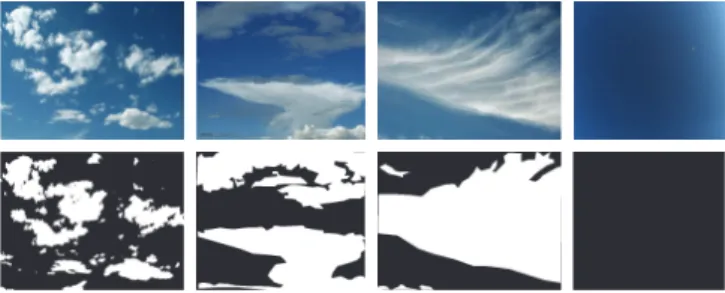
To our knowledge, the only currently available database for sky/cloud images with segmentation ground truth is the HYTA database [6]. It consists of 32 distinct images of vari-ous sky/cloud conditions. Fig. 1 shows a few sample images of the HYTA database along with their corresponding binary ground truth.

Fig. 1: Sample images (top row) along with corresponding sky/cloud segmentation ground truth (bottom row) from the HYTA database.

3.2. Distribution Bimodality

The segmentation of input image into two classes (sky and clouds) becomes easier for those color channels which exhibit higher bimodality. The bimodal behavior of a color channel for the concatenated distribution is measured using Pearson’s Bimodality Index (PBI) as described in Section 2.2. The re-sults are summarized in Table 2. Out of the 16 color chan-nels,c5(S),c1(R), andc13(R/B) have the lowest PBI and thus exhibit the most bimodal distributions, indicating that the segmentation of images into two distinct classes should work well in these color channels.

c1 2.24 c4 3.11 c7 2.71 c10 2.86 c13 2.27 c16 4.27

c2 2.83 c5 1.94 c8 3.98 c11 8.85 c14 4.43

c3 3.25 c6 3.26 c9 5.96 c12 4.59 c15 2.92

Table 2: PBI values for all color channels. The most bimodal channels are highlighted in bold.

3.3. PCA

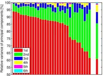
The distribution of the amount of variance captured by the principal components is shown in Fig. 2. The combination of first and second principal components capture a large majority (95.4%) of variance in the input data across the individual images, and over90% for the entire database.

50 55 60 65 70 75 80 85 90 95 100

Relative variance of principal components [%]

1st 2nd 3rd 4th 5th 6th

Fig. 2: Distribution of the variance across the principal com-ponents for all images of the HYTA database. The separate bar on the right shows the variance distribution for the con-catenation of all images of the entire database.

In order to find the most significant vector for the detec-tion of clouds, the contributing effect of the individual vari-ables on the primary principal component axis is analyzed. Every color channel has different loading factors on the most

important principal component axis, and consequently each of them has a different contribution to the common variance captured in the corresponding data matrixX¨i. These

individ-ual loading factors are essentially the projections of the input vectors (color channels) on the principal components. The significant color channels in terms of relative contribution to the first principal component axis arec13(R/B),c15(B_B−₊R_R, andc5(S).

Extending our analysis to finding the most significant pair of color channels, we need to understand a pair’s cumulative contribution to the common variance. The sum of the squares of the corresponding loading factors for different color chan-nels in the concatenated distribution represents the cumulative common variance captured by the pair. The pairs that have the highest cumulative loading on the first principal component arec13-c15,c5-c13, andc5-c15.

Another aspect to consider is the orthogonality between the individual color channels. For this purpose, we compute the triangular area enclosed by two given input vectors (color channels) projected on the plane spanned by the first and sec-ond principal components. There are 162

= 120 combina-tions of two color channels. The triangular area for all unique cases is shown in Fig. 3, where the brightness of each square represents the area captured by the corresponding pair. As expected, certain color channel pairs (the dark patches) are highly correlated, for example the green channel (c2) with most luma channels (c7,c10), the variousR-Bcombinations (c13₋15) with one another, and so on.

c1 c₁ c2 c₂ c3 c₃ c4 c₄ c5 c5 c6 c₆ c7 c₇ c8 c₈ c9 c₉ c10 c₁₀ c11 c11 c12 c₁₂ c13 c₁₃ c14 c₁₄ c15 c₁₅ c16 c16 0.03 0.06 0.09 A B O P rincipal C omponent 1 Pr in ci pa l Co mp on en t 2

Fig. 3: Distribution of area AOBfor all input vector pairs, whereOAandOBare two color channels. The brightness of each square represents the area captured by the corresponding pair.

3.4. Clustering

In order to verify the efficacy of specific color channels in the detection of cloud pixels, 1D and 2D clustering results are presented across all 16 color channels for all the images of HYTA and evaluated using precision, recall, and F-score. Since the ground truth provided by the HYTA database are binary images consisting of two classes, namely sky and cloud, we convert the probabilistic distribution of cloud pix-elspr(xs)(cf. Section 2.4) to a binary image by thresholding,

i.e. a pixel having a probability of cloud>50%is assigned to a cloud pixel and others to sky pixels.

There are 16 color channels for 1D clustering. In a similar manner, there are 162

unique color channel combinations for 2D-clustering. Their performance is illustrated in Fig. 4 in an upper-triangular grid, where the intensity of a particular grid denotes the F-score of that particular color channel pair; the diagonal elements represent the F-scores of the correspond-ing 1D color channels. The most promiscorrespond-ing color channels for 1D-clustering arec13(R/B),c15(_BB₊−R_R), andc5(S) with high precision, recall, and F-scores. For 2D, the best combi-nations includec5-c8,c8-c13, andc8-c15(c8representing es-sentially another variety of red-blue difference), with several other close contenders.

c₁ c 1 c₂ c 2 c₃ c₃ c₄ c₄ c₅ c 5 c₆ c 6 c₇ c₇ c₈ c₈ c₉ c 9 c₁₀ c 10 c₁₁ c₁₁ c₁₂ c₁₂ c₁₃ c₁₃ c₁₄ c 14 c₁₅ c 15 c₁₆ c₁₆ 0.87 0.87 0.87 0.86 0.85 0.85 10 20 30 40 50 60

Fig. 4: F-Scores for all unique cases of 1D (along the diago-nal) and 2D clustering, represented on a brightness scale. The highest F-Scores for 1D (dotted frames) and 2D cases (bold frames) are indicated numerically.

3.5. Discussion

The clustering results as illustrated in Section 3.4 confirm the efficacy of the color channels determined earlier in Section 3.3. Color channelsc5(S),c1(R), andc13(R/B), which

ex-hibit a highly bimodal behavior, are relatively good indicators of clustering performance. We also found the loading factors of the first eigenvector (i.e. the re-projection of the data points on the first principal component) to be a reasonable guide for the choice of good color models; the goodness of fit between loading factors and corresponding F-scores from clustering is high (R2

=0.62).

The pairsc13-c15,c5-c13andc5-c15that came out on top in Section 3.3 also rank highly in terms of 2D-clustering per-formance. However, there is hardly any performance gain from using two color components rather than just one.

As a final comparison, the precision, recall, and F-scores of the best color channels are plotted in Fig. 5 against the out-put of a recently proposed cloud detection algorithm [6]. The data show that a basic 1D clustering method on the most suit-able color components and without any tuning or adaptation can achieve a performance that is on par with a much more complex state-of-the-art sky/cloud segmentation method.

c13 c8−c13 HYTA 0.76 0.78 0.8 0.82 0.84 0.86 0.88 0.9 0.92 0.94 0.96 Precision Recall F−Score

Fig. 5: Precision, recall and F-scores for 1D and 2D cluster-ing compared with a state-of-the-art cloud/sky segmentation algorithm [6].

4. CONCLUSIONS

We presented a systematic analysis of color channels for the detection of clouds from sky/cloud images using distribution bimodality, PCA, and clustering. Experimental evaluation with a cloud segmentation database yields consistent results across analysis methods. Clustering results obtained using the best 1D color channels or 2D color channel pairs (includ-ing red-blue combinationsR/B and B−R

B+R, saturation S, or

in-phase componentI) are on par with the performance of a current state-of-the-art cloud detection algorithm in terms of precision, recall, and F-scores. Future work will involve the additional use of texture and other features to classify clouds into different genera as identified by World Meteorological Organization.

5. REFERENCES

[1] Jun Xiang Yeo, Yee-Hui Lee, and Jin Teong Ong, “Per-formance of site diversity investigated through radar de-rived results,” IEEE Transactions on Antennas and Propagation, vol. 59, no. 10, pp. 3890–3898, 2011. [2] Janet E. Shields, Monette E. Karr, Richard W. Johnson,

and Art R. Burden, “Day/night whole sky imagers for 24-h cloud and sky assessment: History and overview,”

Applied Optics, vol. 52, no. 8, pp. 1605–1616, 2013. [3] M. P. Souza-Echer, E. B. Pereira, L. S. Bins, and

M. A. R. Andrade, “A simple method for the assess-ment of the cloud cover state in high-latitude regions by a ground-based digital camera,”Journal of Atmospheric

and Oceanic Technology, vol. 23, no. 3, pp. 437–447,

2006.

[4] Charles N. Long, Jeff M. Sabburg, Josep Calbó, and David Pagès, “Retrieving cloud characteristics from ground-based daytime color all-sky images,” Journal of Atmospheric and Oceanic Technology, vol. 23, no. 5, pp. 633–652, 2006.

[5] Soumyabrata Dev, Florian M. Savoy, Yee Hui Lee, and Stefan Winkler, “WAHRSIS: A low-cost, high-resolution whole sky imager with near-infrared capabil-ities,” inProc. SPIE Infrared Imaging Systems, 2014, vol. 9071.

[6] Qingyong Li, Weitao Lu, and Jun Yang, “A hybrid thresholding algorithm for cloud detection on

ground-based color images,” Journal of Atmospheric and

Oceanic Technology, vol. 28, no. 10, pp. 1286–1296,

2011.

[7] Josep Calbó and Jeff Sabburg, “Feature extraction from whole-sky ground-based images for cloud-type recogni-tion,”Journal of Atmospheric and Oceanic Technology, vol. 25, no. 1, 2008.

[8] A. Heinle, A. Macke, and A. Srivastav, “Automatic cloud classification of whole sky images,” Atmospheric

Measurement Techniques, vol. 3, pp. 557–567, 2010.

[9] Sylvio Luiz Mantelli Neto, Aldo von Wangenheim, Enio Bueno Pereira, and Eros Comunello, “The use of euclidean geometric distance on RGB color space for the classification of sky and cloud patterns,” Journal of Atmospheric and Oceanic Technology, vol. 27, no. 9, pp. 1504–1517, 2010.

[10] Thomas R. Knapp, “Bimodality revisited,” Journal of Modern Applied Statistical Methods, vol. 6, no. 1, 2007. [11] James C. Bezdek, Robert Ehrlich, and William Full, “FCM: The fuzzy c-means clustering algorithm,” Com-puters & Geosciences, vol. 10, no. 2, pp. 191–203, 1984. [12] C. V. Jawahar, P. K. Biswas, and A. K. Ray, “Inves-tigations on fuzzy thresholding based on fuzzy cluster-ing,” Pattern Recognition, vol. 30, no. 10, pp. 1605– 1613, 1997.