Distributed Thermal Aware Load Balancing for Cooling of Modular Data Centres

(1)

Distributed Thermal Aware Load Balancing

for Cooling of Modular Data Centres

Joseph Doyle

a

, Florian Knorn

b

, Donal O’Mahony

a

, Robert Shorten

b

a_{CTVR, Trinity College Dublin, Ireland}

b_{Hamilton Institute, National University of Ireland, Maynooth, Ireland}

Abstract

Thermal management in data centres requires a complicated trade-off between cooling costs and thermally induced equipment failure rates. Using ideas from cooperative control and distributed rate limiting, in this paper we describe a distributed architecture that can be used for thermal aware load balancing for a common type of modular data centre; namely an algorithm that, for a given demandD∗

, distributes load to individual machines such that the temperatures in the individual modules are equalised. The benefit of shifting load based on thermal considerations is that significant gains in cooling cost can be achieved. We evaluate the performance of the algorithm using computational fluid dynamics (CFD) and Matlab simulations. Our results show that significant cost savings can be made by applying such algorithms, and that these can be achieved without the need for detailed modelling and tuning of controllers.

Key words: thermal equilibrium; Load balancing algorithms; stability; distributed control; computational methods

1 Introduction

In this study we examine air temperature manage-ment in buildings and data centres. A data centre is a warehouse-scale building which may contain up to tens of thousands of high performance servers as well as the 5

associated networking and cooling equipment, thereby producing large amounts of heat as they perform their tasks. In large scale data centre operations, the mod-ular data centre approach is becoming more and more popular, [6]. Such data centres are built from a number 10

of independent, autonomous modules (typically housed in standardised overseas shipping containers), that each contain a large number of servers. Computer room air conditioning (CRAC) units are used to extract heat coming from the servers, cool it, and provide the cooled 15

air back to their inlets, so as to prevent equipment dam-age. Cooling equipment is clearly crucial to long-term reliability of operation; it has been shown for instance that every 10◦_C _{increase above} ₂₁◦_C _{decreases the}

long-term reliability of electronics by 50% [13]. In addi-20

⋆

Email addresses: [email protected](Joseph Doyle), [email protected](Florian Knorn),

[email protected](Donal O’Mahony), [email protected](Robert Shorten).

tion, a15◦_C_{rise increases the failure rates of hard disk}

drives by a factor of two [2]. It is also possible to use water cooling in data centres [20,1] but the majority of data centres use air cooling.

The cost of providing cool air to the server inlets can 25 be considerable. Consider a30,000 ft2data centre with 1000 standard computing racks, each consuming10 kW. With an average electricity cost of$100/MWh the an-nual cooling cost would be in the order of $4–$8 million, [17]. It is thus clearly in the interest of the data centre 30 operator to operate the facility as eﬃciently as possible to minimise such costs. Similar problems also arise else-where, for example in thermal management of buildings. Initiatives such as IBM’s “Smart Cities” program have been created with this and similar management prob- 35 lems in mind.

Our objective in this paper is to address thermal man-agement in a data centre which utilises modular data centre components. Note that there have been numerous proposals for the thermal management of servers in data 40 centres [21,13,8,16]. A notable deviation to this work [9], considers a combination of the cooling power for CRAC units and the idle and dynamic power of servers in a load balancing scheme to lower overall energy costs. While this appears to be a new approach to the problem, in this 45 paper we consider the traditional approach to achieve

(2)

cost of minimisation. In addition, there is an increased trend toward energy proportional servers [4] which rep-resent advanced servers where the idle power is virtually zero and the idle power of servers is likely to be less im-portant in the future. All of these proposals, however, 5

rely on a central scheduler, which is both a bottleneck for control messages and a single point of failure. Such central solutions typically require lengthy calibrations to minimise operational costs. A distinctive feature of the present work, however, is that we would like to pro-10

pose a robust distributed algorithm which attempts to reduce cooling costs, prevents equipment damage while satisfying demand requirements, all without the need of detailed calibrations. Such an algorithm would, with its plug & play functionality, be eminently applicable in a 15

modular environment. Speciﬁcally, the contributions of this paper are as follows:

• We present a distributed algorithm to both regulate total demand serviced to a certain given level, sub-ject to the additional constraint that temperature is 20

equalised amongst all machines.

• In certain situations, when more demanding require-ments are placed on the data centre, we show that ex-isting algorithms from communication networks can be applied in this context.

25

• Finally, data from an industry standard computa-tional ﬂuid dynamic (CFD) Flovent [7] is used to validate the algorithms.

The performance of the proposed algorithms in minimis-ing the total coolminimis-ing cost is evaluated. It will be shown 30

that the total cooling costs can be reduced signiﬁcantly while servicing a desired demand.

The application described in this paper uses algorithms ﬁrst described in [11] and [22]. The speciﬁc contribution of this work is to apply and develop the ideas in these pa-35

pers to problems arising in thermal management of data centres. A detailed mathematical analysis of these algo-rithms is given in the aforementioned papers. Hence, in the sequel, we give only very brief mathematical details.

2 Preliminaries

40

We shall study thermal management in the context of a large scale data centre. In the following, we shall use the term “machine” in a rather abstract sense in that we as-sume that each “machine” actually consists of a housing that contains a large number of individual servers which, 45

jointly, have a cooling facility associated with them. This assumption is justiﬁed, for instance, by the increasingly popular modular data centres, where large clusters of servers are housed in autonomous shipping containers that are all connected to a common chilled water supply, 50

[6]. Such a container would then be considered a “ma-chine” in the context of this paper.

2.1 Problem setting

We now consider a data centre that is constructed using

nmachines. Each machinei∈ {1,2, . . . ,n} has, at time 55

k = 0,1,2, . . ., an inlet temperature (or just “tempera-ture”) ofTi(k), which represents the temperature of the

air sucked into the servers for cooling. We assume that this temperature is the same for all the servers inside a given machine; this assumption is justiﬁed in partic- 60 ular when suitable cold aisle containment is used inside the machine (Our simulations show that the largest dif-ference in temperature between the inlets of servers is 0.3◦_{C). In addition, simulation 3 examines how much}

the demand of neighbouring server racks affects the tem- 65 perature. Furthermore, even in the presence of this de-fect the algorithm works well. Note our simulations are based on Flovent [7], an industry standard simulator, and these simulations indicate that even in the presence of this effect, the algorithm is efficacious. We also assume 70 that there is sufficient distance between the machines that heat exchanges can be neglected and that these are cased and isolated from each other. Recall that machines refer to housings that contain a large number of individ-ual servers. Additionally, each machine is servicing a de- 75 mand (also referred to as “work load”) ofDi(k), so that

the total demand serviced by the data centre at timekis

D(k) :=X

i

Di(k) (1)

An important feature of our work is that the total de-mandD(k)is regulated to some desired valueD∗_{, which}

may be time-varying (for notational convenience, we 80 omit the dependence ofD∗_on_k_{). Hence, the value of the}

total demand serviced and its deviation from D∗ _must

be known either implicitly or explicitly by at least one machine in the data centre.

Given a constant amount of cooling energy supplied to 85 each machine, the temperatures inside each machine will be a direct function of the demand serviced by that ma-chine (since the heat energy dissipated by the CPUs is roughly proportional to the amount of work done by the CPUs). Borrowing from the terminology established in 90 [11], this interdependency is described by the “utility functions”, which relate the “physical state” (demand)

Di of machineito its “utility value” (temperature):

Ti=fi(Di) (2)

Note thatfiis typically non-linear and is used to model

complicated ﬂuid dynamic eﬀects as well as natural cool- 95 ing within the machines. We assume that the manner in which workload is distributed inside the machines is uniform.

Next, we assume that a limited information exchange between machines is possible. Speciﬁcally, at timek, ma- 100

(3)

chinei can provide information about itself (in partic-ular its current temperature) to another machine j if and only if (i,j) is an arc in the directed communica-tion graph G(k) = N,E(k)

, which thus describes the topology of the possible information exchange between 5

machines. This graph is allowed to change over time and is assumed to be jointly strongly connected over a given, ﬁxed time horizon m ≥ 1. By this, we mean that ev-ery union ofmconsecutive graphs is assumed to yield a strongly connected graph.1

10

We would now like to ﬁnd an algorithm that will attempt to equalise the temperatures among machines, while en-suring that some desired demand D∗ _{is being serviced}

by the data centre.

2.2 A cooperative control scheme (Algorithm 1) 15

The recent publication [11] gives an in-depth discussion of three iterative algorithms and variations thereof that are designed to allow a network to achieve a common goal cooperatively while satisfying certain local constraints. The data centre load balancing problem ﬁts into this 20

framework and we shall now reproduce, for convenience, some of the mathematical statements from this publica-tion (in particular Theorem 4.1).

To apply these results, we must assume that the util-ity functions are continuous, monotone functions with 25

bounded growth rates (to guarantee feasibility of the so-lution) and that each machine has knowledge of the to-tal demand being serviced by the data centre. Note it is also assumed that the update law for the algorithm uses a time scale that is larger than that of the dynamics of 30

the settling time for the temperatures; namely that the relationship betweenDiandTican be adequately

mod-elled using a static map. Given these assumptions, the following theorem (adapted from Theorem 4.1 in [11]) provides a stable update law to iteratively reﬁne the de-35

mands being serviced by the individual machines so that the data centre converges to the desired behaviour:

Theorem 1. For some initial condition Di(k = 0)

and any sequence of strongly connected communication graphs, suppose that the machines iteratively update 40

their work load according to

Di(k+1) =Di(k)+

X

(j,i)∈E(k)

ηij(k) Tj(k)−Ti(k)+µ(k)σ(k)

(3)

1 _{The union of a set of graphs on a common vertex set is} defined as the graph consisting of that vertex set and whose edge set is the union of the edge sets of the constituent graphs. where σ(k) =      D∗₋ n X i=1 Di(k+1−M) ifk+1is a multiple ofM 0 otherwise (4) withM:=n−1. If the gains satisfy

0< µ≤µ(k)≤µ¯ and 0< ηi≤ηij(k)≤η¯i (5)

then — provided µ >¯ 0 and η¯i > 0 are sufficiently

small — the demandsDi(k)converge asymptotically to 45 valuesD∗

i for whichfi D∗i

=T∗_{for all}_i_{= 1}_{, . . . ,n}_and P

iD

∗

i =D

∗_.

For a proof of the Theorem and a much more detailed description of the mathematical assumptions therein,

please refer to [11]. 50

Comment. Explicit bounds onη¯iandµ¯are also given

in [11]. While for the purpose of proving convergence in the theorem small values of these constants are required, in practical situations it is found that they can be sig-niﬁcantly larger. Mathematical details are given in [11]. 55 These are quiet involved and are beyond the scope of the present paper. Roughly speaking, the stability con-ditions are based on connectivity arguments in graphs. As the graphs become large, then these conditions give small controller gains. This approach does not account 60 for structural properties of the graph and consequently may be quite conservative.

The update law (3) from the Theorem, which we will re-fer to as Algorithm 1, thus provides a rule specifying how to iteratively update the load on the machines to bal- 65 ance the temperatures among the machines in the net-work. It basically consists of two intuitive-to-understand parts: The first part, summing over the differences in temperatures between neighbours, is aimed at reducing the temperature differences; if, for instance, all neigh- 70 bouring machines of machineiare operating cooler than machinei, then it should reduce its own demand in or-der to approach the temperature level of the surround-ing machines. The second part in the equation is to en-sure that the global demand is satisfied. It is easy to 75 see that if the total demand serviced by all the ma-chines is below the required quantity, then each machine should increase their own work load somewhat so that the network, jointly, increases the demand serviced until

it reaches the desired level. 80

The pseudocode shown in Figure 1 describes an imple-mentation of this algorithm.

2.3 A notable simplification (Algorithm 2)

In situations where the communication graph is undi-rected, where the total required demand is not subject to 85

(4)

1 UpdateDemand()

2 Once every∆units of time do 3 fori= 1 :n 4 Di←Di+ηP_(i,j)∈E Tj−Ti 5 ifmod(k+ 1, n−1) == 0 6 Di←Di+µσ 7 endif 8 endfor 9 ifmod(k+ 1, n−1) == 0 10 σ← D∗ −Pn i=1Di 11 endif 12 k←k+ 1 13 enddo 14 InitialiseDemand() 15 k←0 16 σ←0 17 fori= 1 :n 18 Di←D∗/n 19 endfor

Figure 1. Pseudocode for Algorithm 1.

1 UpdateDemand()

2 Once every∆units of timedo

3 fori= 1 :n 4 Di←Di−ηP₍_i,j₎_∈E(Ti−Tj) 5 endfor 6 k←k+ 1 7 enddo 8 InitialiseDemand() 9 k←0 10 fori= 1 :n 11 Di←D∗/n 12 endfor

Figure 2. Pseudocode for Algorithm 2.

change, and where the utility functions satisfy stronger assumptions, then considerable simpliﬁcations are pos-sible. In particular, the algorithms given in [22] apply. Speciﬁcally, suppose that: (a) the communications graph is undirected; (b) the desired demand D∗ _{is constant;}

5

(c) the utility functionsfi :R→Rare increasing,

con-cave, diﬀerentiable functions, and have continuous ﬁrst derivatives. Then the algorithm described by the pseu-docode in Figure 2 may be used to solve the thermal management problem posed above.

10

The basic idea encapsulated above is as follows. Initially, the demand is divided evenly among the server racks. The demand Di of each machine i is then iteratively

updated with a term that is proportional to the sum over the diﬀerences between the own temperature and that 15

of neighbouring racks, that is

D1(0) =D2(0) =. . .=Dn(0) (6a) Di(k+ 1) =Di(k)−η X (i,j)∈E Ti(k)−Tj(k) (6b)

The gain parameterηdetermines the responsiveness and stability of the algorithm and its choice is discussed in [22]. The stability and convergence properties are cap-tured by the following theorem, cf. [22]. Before stating 20 this theorem, we need to establish some further termi-nology. Denote bygi=fi−1the inverse functions of the

fi, which must exist given the convexity and

diﬀeren-tiability assumption above. Note also, due to symmetry, the system given by (6) satisﬁes the demand constraint 25 (1) for allk= 0,1,2, . . ..

Theorem 2. Let di be the degree of node iin the

com-munication graph. Ifη satisfies:

0< η < 1 21min≤i≤n h −gi′ Ti(0) i min 1≤i≤n 1 di , (7)

then the system given by(6)will converge to lim k→∞Di(k) =D ∗ i withP iD ∗ i =D, and 30 lim k→∞Ti(k) =T ∗ for alli= 1, . . . ,n. Proof. See [22].

∆is indeed related to the settling time associated with thefi()functions. In the original work on this topic [11],

these functions are static maps where as in this appli- 35 cation this is not entirely true. Our basic assumption is that the dynamics associated with thefi()functions are

fast when compared with the update law. Of course this assumption has to be validated experimentally and the step size determined empirically. For our simulation∆ 40 was always chosen to be much larger than the dynamics associated with thefi()functions. Recall the objective

of this paper was illustrate the use of a new and innova-tive distributed control algorithm developed in [11] for this novel application. In our CFD simulations each it- 45 eration of the Flovent software was run every∆seconds.

Comment. Before proceeding to evaluate in simula-tion the algorithms described in this paper, we note here that the decentralised control advocated in this paper is motivated by recent developments in consensus algo- 50 rithms and in gossiping algorithms. In this context it

(5)

may be viewed as a somewhat non-traditional approach to decentralised control systems. The interested reader is referred to the work of Jadbabaie et al.[10], Olfati-Saber and Murray [15], Linet al.[12] and Moreau [14] for initial ideas in this direction. More recent developments 5

were presented by Knornet al.[11] as well as Stanojević and Shorten [22]. These later articles provide much of the theoretical framework for the speciﬁc work described in this paper.

3 Simulation and validation

10

To evaluate the performance of the algorithms we used a CFD simulator. Three simulations were conducted. In the ﬁrst simulation, we consider a data centre with twelve machines of three diﬀerent types (that is, four machines of each type). Data from the CFD simulator 15

was used to generate the utility functions, andMatlab based simulations were then used to evaluate the ability of Algorithm 1 to track a given time-varying demand. We then repeat this simulation, using Algorithm 2, in the case where the communication graph is undirected 20

and the demand is fixed. Finally, we then apply Algo-rithm 2 to a conventional (non-modular) data centre, where “machines” are now represented by server racks inside a single room. In this situation, to capture the ex-tremely complicated fluid dynamic effects, the full simu-25

lation was carried out using the CFD simulator. Finally note that while the gains in each situation may be cho-sen in accordance with the bounds given in Theorems 1 and 2 (and the respective references), larger values were in fact used to speed up convergence for the purpose of 30

exposition.

3.1 Simulation setup

Our simulation setup follows that used in [21,13]. Each machine (data centre) used in this study has dimen-sions 11.7 m×8.5 m×3.1 m with a 0.6 m raised ﬂoor 35

plenum that supplies cool air through perforated ﬂoor tiles. There are four rows of servers with seven 40 U racks in each case, resulting in a total of 1120 servers. The dimensions of the server racks are depicted in Fig-ure 3(a). Note the front and rear doors were removed to 40

allow the air to ﬂow freely. The servers simulated were based on Hewlett-Packard’sProliant DL360 G3smodel, which consumes150 Wof power when idle and285 Wat 100% utilization. From this we could determine that the total power consumption of the data centre is 168 kW 45

(40×28×150 W) when idle and 319.2 kW (40×28×

285 W) at full utilisation. The ﬂow rate of the server rack was 1,500 ft3/min representing 40 servers with a ﬂow rate of37.5 ft3/min. We also used an idealenergy proportional version of said server, [4]. Recall that these 50

represent advanced servers where the idle power is vir-tually zero.

A

B

C

D

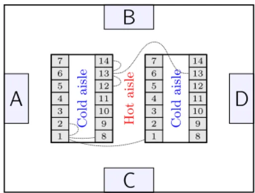
1 2 3 4 5 6 7 1 2 3 4 5 6 7 8 9 10 11 12 13 14 8 9 10 11 12 13 14 H o t a is le C o ld a is le C o ld a is le

Figure 4. Layout of simulation setup. To illustrate the com-munication graphs used in simulation 3, the dotted lines in-dicate which other machines the racks 1 and 13 from the left cold aisle can exchange temperature information with. Server racks in adjacent aisles are connected to lower tem-perature differences between aisles.

For cooling, the data centre is equipped with four CRAC units “A_{”, “}B_{”, “}C_{” and “}D_{” whose locations are also}

in-dicated in Figure 4. Each CRAC unit pushes air chilled 55 to 15◦_C _{into the plenum at a rate of} ₁₀_,_{000 ft}3_/_min. The cooling capacity of the each CRAC unit is limited to 90 kW, and in full operation each CRAC unit itself consumes 10 kW. Flovent basically uses a k-ǫ turbu-lence model; see documentation describing mathemati- 60 cal modelling given as part of [7]. The air velocity, pres-sure and turbulence at the front boundary of the server racks are depicted in Figure 3(b), 3(c) and 3(d). CFD simulations are now used routinely in data centre design and have been found be to very useful by practising en- 65 gineers. There is, however, a need for detailed validation against experimental data. These concerns, however, are not addressed in this paper and CFD simulations are car-ried out using the popular commercial package Flovent. Given this simple setting, we now describe three basic 70 variations that may arise. In the ﬁrst case, the machine is exactly as described above with the standard HP servers. This type is hereafter referred to as “NC-NF". For the second case, we decided to model the machine using a “cold aisle containment” assumption, [19] with CRAC 75 unitD_{oﬄine. Recall that cold aisle containment refers}

to the segregation of the cold aisle from the rest of the data centre using physical barriers such as PVC curtains or Plexiglas [5]. This type of data centre is likely to be-come more and more popular in the future, [18]. This 80 type is hereafter referred to as “C-F". It is also possible to use “hot aisle containment" which is the segregation of the hot aisle from the rest of the data centre. While there is some evidence that “hot aisle containment" may be a more efficient design, it is recognised [18] that there 85 are difficulties in retrofitting this solution which may make “cold aisle containment" the more popular design, at least in the short-term. The third case is identical to the second case, but servers of the energy proportional type were used. This type is hereafter referred to as “C- 90 F-P". Each case has a utility function associated with it

(6)

S

er

ve

rs

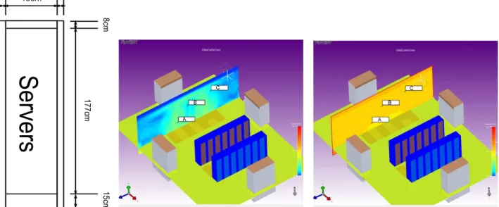
6cm 6cm 48cm 15cm 17 7cm 8cm

(a) Geometry of the server rack. All components in the server rack are 60cm thick.

A B

C

(b) Air velocities in front of the server rack. At point A the air velocity is1.18 m/s. The air velocity at point B is0.38 m/sand at point C the air velocity is0.622 m/s.

A B

C

(c) Pressure conditions in front of the server racks. At point A the pressure is −2.75 Pa. The pressure at point B is −0.61 Paand at point C the pressure is−1.13 Pa.

A B

C

(d) Turbulence in front of the server racks. The turbulence at point A is0.0337 J/kg. At point B the turbulence is0.0102 J/kgand the turbulence at point C is0.01 J/kg

Figure 3. Geometry of the server rack as well as the air velocity, pressure and turbulence conditions in front of the server racks that describes the relationship between load and

maxi-mum inlet temperature found inside the machine. These utility functions, which we shall later use in our simula-tions, are depicted in Figure 5.

In order to evaluate the performance of the algorithms 5

we need to be able to calculate the cooling costs. Let

Q be the amount of power the servers consume, Tsup

the temperature of the air that the CRAC units sup-ply, Tsafe = 25◦Cthe maximum permissible

tempera-ture at the server inlets in order to prevent equipment 10

damage, Tmax the maximum temperature of the server

inlets in the machine and Pfan the power required by

C-F-P C-F NC-NF CPU usage Tma x 0 15 30 45 60 75 10 30 50 70

(7)

the fans of the CRAC units. The “coeﬃcient of perfor-mance” (COP), that is the ratio of heat removed to work necessary to remove the heat, is a function of the supply temperatureTsupbeing provided by the CRAC. There is

considerable debate over the maximum permissible tem-5

perature at the inlet in order to prevent equipment dam-age. While there is a guidelines in this area it has changed recently [3] and we selected the valueTsafe= 25◦Cas it

is a well established value which has been used in other systems [21,13]. The cooling costC can then be calcu-10

lated as:

C= Q COP(Tsup)

+Pfan (8)

If the highest temperature found at any inlet in the data centre is below the “red-line” temperature, then the CRAC is cooling the data centre excessively. In such a situation, the supply temperature can be raised by 15

Tsafe−Tmax (by reducing the amount of cooling) to

re-duce costs while still observingTsafe.

Comment. While other factors such as complex non-linear flow effects and the cost of pumping air to difficult-to-reach parts of the data centre affect the cooling cost, 20

the highest machine temperature is a major factor in the cooling cost. This observation is what motivates us to equalise temperatures.

If, in turn,Tsafe−Tmaxis negative the equipment is in

dan-ger of being damaged and the supply temperature must 25

be lowered in order to cool down the machine responsi-ble forTmax. In our simulations, to determine this

max-imum inlet temperature, we used the commercial CFD simulator Flovent_{. Each of the four CRAC fan units} consumed10 kWso that for each machinePfan= 40 kW

30

and Tsup = 15◦C. The COP curve used to calculate

the cooling costs is a standard curve for a water chilled CRAC and is given in [13].

3.2 Simulation 1

As mentioned above, the setup for this simulation con-35

sists of a modular data centre site housing twelve ma-chines (containers), four of each type described above. Our objective in the following is to regulate the aggre-gate CPU load to three levels: 40%, then 55% and ﬁ-nally 25% in a situation where the resulting communi-40

cation network is strongly connected, but chosen ran-domly. The resulting evolution over time of the aggre-gate demand, individual demands and individual tem-peratures are given in Figure 6. The simulations are mea-sured in terms of iterations for reasons which are dis-45

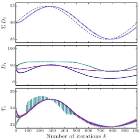
cussed in Section 2.3. As can be seen, the cost savings achieved in the equilibrium for the 40% level are signif-icant when compared to the initial temperature conﬁg-uration. The maximum rack inlet temperature drops by approximately 1◦_C _{and consequently the cooling cost}

50

drops from1.514 MWto1.416 MW, yielding a 6.5%

re-Number of iterationsk Ti D i Σ D i 0 100 200 300 400 500 600 700 800 900 1000 22 25 28 0 50 100 25 40 55

Figure 6. Performance of Algorithm 1 at three demand levels

D∗

={40%,55%,25%}, which are indicated by the dashed line in the top plot, usingη= 0.1,µ= 1/3.

Number of iterationsk Ti D i Σ D i 0 100 200 300 400 500 600 700 800 900 1000 22 24 26 0 50 100 25 40 55

Figure 7. Performance of Algorithm 1 with demand varying in a periodic fashion, usingη= 0.1,µ= 1/3.

duction in the cooling costs. This represents a saving of tens of thousands of dollars annually.

Comment. As the equilibrium state is achieved for any randomly connected graph, these cost savings are 55 robust with respect to changes (such as link failures) in the communication topology.

Finally, Figure 7 depicts a scenario where the demand is varying in a periodic fashion; for example daily de-mand patterns are often assumed to be periodic. As can 60 be seen, satisfactory tracking is achieved even though Algorithm 1 is designed for ﬁxed point regulation only.

(8)

Number of iterationsk Ti D i Σ D i 0 50 100 150 200 250 22 23 24 0 50 100 38 40 42

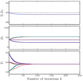
Figure 8. Performance of Algorithm 2 with constant demand of 40%, usingη= 0.1. Number of iterationsk Ti D i Σ D i 0 50 100 150 200 250 22 23 24 0 50 100 38 40 42

Figure 9. Performance of Algorithm 2 with a single broken link and constant demand of 40%, usingη= 0.1.

3.3 Simulation 2

The setup is exactly as before. However, we now enforce the additional assumptions made in Sec. 2.3; recall in particular the assumption of symmetry in the informa-tion exchange. Figure 8 depicts Algorithm 2 equalising 5

temperatures for a constant total load of 40%. Note, however, the eﬀect of breaking a single link. As can be seen in Figure 9, the total demand constraint can no longer be satisﬁed and the site cannot satisfy the most basic quality of service requirement, namely that all re-10

quests are answered. Note that this is not surprising since the algorithm was never designed to operate in such a scenario. 16 18 20 22 24 0 1 2 3 4 5 6 7 8 Temperature Number of Iterations

Figure 10.η = 13. The temperature of inlets of the server racks at each iteration of Algorithm 2 inside a modular data centre.

3.4 Simulation 3

A basic criticism of the discussion thus far may con- 15 cern the type of data centre site considered. In many situations the assumption of containment is not valid. Namely, thatTiof machineidepends not only onDibut

also potentially onDj(j6=i) and assumption regarding

the lack of heat exchange between machines is removed. 20 Surprisingly, the algorithm works well in this case also. In such situations it is of interest to observe the perfor-mance of the algorithms presented above. To conclude this paper, we brieﬂy apply Algorithm 2 to one such sit-uation. Similar results can be expected for Algorithm 1 25 also.

Let us now consider a single machine as described above, in particular of type 3. Then assume that the server racks inside are labelled in pairs “1” to “14” as shown in Figure 4. While any connected communication graph 30 could be used in our algorithm, we chose the following topology for G: Let each server rack be connected to its immediately adjacent server racks and to the server rack with same label in the other cold aisle. Server racks labelled “1” and “7” are connected to server racks di- 35 rectly opposite them across the cold aisle (that is, “8” and “14” respectively). Clearly, this results inGbeing a connected, undirected (3-regular) graph. As can be seen from Figure 10, even in this non-ideal scenario, Algo-rithm 2 still manages to, more or less, equalise the tem- 40 peratures across server racks. Note ﬁnally that this sim-ulation is notMatlab_{based but rather a full scale CFD} simulation.

4 Conclusions

Thermal management is an important aspect in the ef- 45 ﬁcient operation of data centres. The relationship be-tween demand and temperature is a complicated one so a robust distributed algorithm is useful in the dynamic

(9)

environment of the data centre. In this paper, we have shown that distributed algorithms can be used to reduce cooling costs in certain types of data centres. A 6.5% re-duction in the cooling costs which represents savings of tens of thousands of dollars annually can be achieved. 5

Future work will explore learning automata ideas in the context of more general data centres.

Acknowledgements

The authors would like to thank Andreas Simon-Kajda and Dirk Niemeier for their help with the CFD simula-tions. This work is partially funded by the Irish Higher Education Authority under the HEA PRTLI Network Mathematics Grant and by SFI grant 07/IN.1/I901.

References

[1] Ali Almoli, Adam Thompson, Nikil Kapur, Jonathan 10

Summers, Harvey Thompson, and George Hannah. Computational ﬂuid dynamic investigation of liquid rack cooling in data centres. Applied Energy, 89:150–155, 2012. [2] Dave Anderson, Jim Dykes, and Erik Riedel. More than an

interface—SCSI vs. ATA. InProceedings of the 2nd USENIX 15

Conference on File and Storage Technologies, pages 245–257, San Francisco, April 2003.

[3] ASHRAE Technical Committee 9.9. 2011 thermal guidelines for data processing environments - expanded data center classes and usage guidance, 2011. 20

http://tc99.ashraetcs.org/documents/ASHRAE

Whitepaper - 2011 Thermal Guidelines for Data Processing Environments.pdf.

[4] L. A. Barroso and Urs Hölze. The case for energy-pro-portional computing. IEEE Computer, 40(12):33–37, 2007. 25

[5] L. A. Barroso and Urs Hölzle. The datacenter as a computer: An introduction to the design of warehouse-scale machines. Synthesis Lectures on Computer Architecture, 2009. [6] Henry C. Coles and Mark Bramﬁtt. Modular/container

data centers procurement guide: Optimizing for energy 30

eﬃciency and quick deployment. Lawrence Berkeley National Laboratory, February 2011. Available at http://goo.gl/ho9cC.

[7] Mentor Graphics Corporation. Flovent version 9.1, 2010. [8] Rajarshi Das, Jeﬀrey O. Kephart, Jonathan Lenchner, and 35

Hendrik Hamann. Utility-function-driven energy-eﬃcient cooling in data centers. In Proceedings of the 7th International Conference on Autonomic Computing, pages 61–70, Washington, June 2010.

[9] Ahmad Faraz and T.N. Vijaykumar. Joint optimization of 40

idle and cooling power in data centers while maintaining response time. InProceedings of ASPLOS, pages 243–256, Pittsburgh, 13 - 17 March 2010.

[10] Ali Jadbabaie, Jie Lin, and A. Stephen Morse. Coordination of groups of mobile autonomous agents using nearest 45

neighbour rules. IEEE Transactions on Automatic Control, 48(6):988–1001, 2003.

[11] Florian Knorn, Martin J. Corless, and Robert N. Shorten. Results in cooperative control and implicit consensus. International Journal of Control, 84(3):476–495, March 2011. 50

[12] J Lin, A S Morse, and B D O Anderson. The Multi-Agent Rendezvous Problem. InProceedings of the IEEE Conference on Decision and Control, volume 2, pages 1508–1513, Maui, 9 - 12 December 2003.

[13] Justin Moore, Jeﬀrey S. Chase, Parthasarathy Ranganathan, 55 and Ratnesh Sharma. Making scheduling “Cool”: Temperature-aware workload placement in data centers. In Proceedings of USENIX, pages 61–75, Anaheim, April 2005. [14] Luc Moreau. Stability of multiagent systems with

time-dependent communciation links. IEEE Transactions on 60 Automatic Control, 50(2):169–182, 2005.

[15] Reza Olfati-Saber and Richard M. Murray. Consensus protocols for networks of dynamic agents. In Proceedings of American Control Conference, volume 2, pages 951–956, Denver, 4 - 6 June 2003. 65 [16] Luca Parolini, Niraj Tolia, Bruno Sinopoli, and Bruce H.

Krogh. A cyber-physical systems approach to energy management in data centers. In Proceedings of the 1st ACM/IEEE International Conference on Cyber-Physical Systems, Stockholm, April 2010. 70 [17] Chandrakant D. Patel, Cullen E. Bash, and Ratnesh Sharma.

Smart cooling of data centers. In Proceedings of IPACK, pages 128–137, Maui, 6-11 July 2003.

[18] Michael K. Patterson and Dave Fenwick. The state of datacenter cooling. Available athttp://goo.gl/GUlvF. 75 [19] Mikko Pervilä and Jussi Kangasharju. Cold air containment.

In Proceedings of ACM SIGCOMM Workshop on Green Networking, pages 7–12, Toronto, August 2011.

[20] Peter Rumsey. Overview of liquid cooling systems, 2007. http://hightech.lbl.gov/presentations/Dominguez/ 80 5_LiquidCooling_101807.ppt.

[21] Ratnesh K. Sharma, Cullen E. Bash, and C. D. Patel. Balance of power: Dynamic thermal management for internet data centers. IEEE Internet Computing, 9(1):42–49, 2005.

[22] Rade Stanojević and Robert Shorten. Generalized distributed 85 rate limiting. In Proceedings of IWQoS, pages 1–9, Charleston, July 2009.