Instituut voor Theoretische Fysica
Time, Heat and Work
aspects of nonequilibrium statistical mechanics
Tim Jacobs
Promotor:
Prof. Dr. Christian Maes
Proefschrift ingediend tot het behalen van de graad van Doctor in de Wetenschappen
Introduction 3
1. Thermodynamics and statistical mechanics . . . 3
2. Beyond equilibrium: time enters the play . . . 5
3. Fluctuation relations for work and heat . . . 7
4. A discussion on the results . . . 9
5. Outline . . . 11
1 Describing physical systems 15 1.1 Physical systems . . . 15
1.1.1 Scene . . . 15
1.1.2 Scales of objects and levels of description . . . 16
1.1.3 Minimal requirements for a description of an object . . 17
1.2 The description of classical systems . . . 17
1.2.1 Microstates . . . 17
1.2.2 The microscopic dynamics . . . 18
1.2.3 Distributions on phase space . . . 20
1.2.4 Macrostates . . . 22
1.3 The description of quantum systems . . . 24
1.3.1 Microstates . . . 24
1.3.2 Microscopic dynamics . . . 25
1.3.3 Macrostates . . . 28
1.3.4 Pure states and statistical mixtures . . . 29
1.4 The description of stochastic systems . . . 32
1.4.1 Detailed balance . . . 33
1.4.2 Continuous diffusion processes . . . 34
1.4.3 Elements of stochastic calculus . . . 37
2 Entropy 41 2.1 The trouble with entropy . . . 41
2.2 The definition of entropy . . . 43
2.2.1 The historical definition of entropy . . . 43
2.2.2 Thermodynamic definition of entropy . . . 45
2.2.3 The Boltzmann entropy in classical systems . . . 47
2.2.4 The Shannon entropy in classical systems . . . 52
2.2.6 The Boltzmann entropy in quantum systems . . . 61
2.2.7 The von Neumann entropy in quantum systems . . . 62
2.2.8 The Gibbs-von Neumann entropy in quantum systems . 67 2.2.9 Relative entropy . . . 69
2.3 Entropy as a measure of irreversibility . . . 72
2.3.1 Different kinds of reversibility . . . 73
2.3.2 Time-reversal symmetry breaking and entropy . . . 74
2.4 The second law of thermodynamics . . . 77
2.4.1 The thermodynamic arrow of time . . . 77
2.4.2 Gibbs entropy and the second law revisited . . . 79
2.4.3 A microscopic foundation of the second law? . . . 82
2.4.4 Concluding remarks . . . 84
2.5 Final words on entropy . . . 87
2.5.1 Entropy as a measure of disorder? . . . 87
2.5.2 Entropy is contextual . . . 88
3 Quantum entropy production as a measure of irreversibility 91 3.1 Introduction . . . 91
3.2 Entropy production for a unitary evolution . . . 93
3.2.1 Setting . . . 93
3.2.2 The time-reversal invariant situation . . . 94
3.2.3 The production of entropy . . . 94
3.3 Perturbations by measurement . . . 95
3.3.1 Path-space measure . . . 96
3.3.2 Time-reversal . . . 97
3.3.3 Entropy production . . . 97
3.4 Conclusions and additional remarks . . . 99
4 Aspects of quantum irreversibility and retrodiction 101 4.1 The trouble with irreversibility . . . 101
4.2 Statistical reversibility I . . . 103
4.2.1 The classical realisation . . . 103
4.2.2 The jump to the quantum world . . . 104
4.3 Quantum formalism . . . 105
4.4 Statistical reversibility II . . . 107
4.5 Retrodiction . . . 110
4.5.1 The magic of retrodiction . . . 110
4.5.2 More spectacular examples. . . 111
4.5.3 When retrodiction seems to go wrong . . . 114
4.6 Thermodynamic irreversibility . . . 116
4.7 Conclusions . . . 117
5 An extension of the Kac ring model 119 5.1 Relaxation to equilibrium . . . 119
5.2 The original Kac ring model . . . 120
5.2.1 The Stoßzahlansatz of Boltzmann . . . 120
5.2.3 Discussion . . . 126
5.3 An extension of the Kac ring . . . 127
5.3.1 Hilbert space and notation . . . 128
5.3.2 Dynamics and observables . . . 128
5.3.3 Equilibrium . . . 130
5.3.4 Initial data . . . 131
5.3.5 Autonomy and entropy . . . 132
5.4 Results . . . 133
5.5 Discussion . . . 135
5.5.1 Molecular chaos . . . 135
5.5.2 Autonomous equations andH−theorem. . . 136
5.5.3 Relaxation to equilibrium? . . . 138
5.5.4 Higher spins . . . 138
5.5.5 Kac ring model . . . 139
5.6 Proof of results . . . 140
5.6.1 Equivalence ofǫ-ensembles . . . 140
5.6.2 Typical equivalence of the unitary and reduced dynamics 141 5.6.3 The initial states are dispersion free. . . 144
5.6.4 The relaxation of the magnetization . . . 145
5.6.5 The equilibrium magnetization . . . 146
5.6.6 The calculation of the Gibbs-von Neumann entropy . . 147
5.6.7 Typicality explored . . . 148
5.7 Conclusions . . . 149
6 Fluctuation relations for work and heat 151 6.1 A model to study fluctuations for heat and work . . . 151
6.1.1 The motivation to study fluctuations . . . 151
6.1.2 Setting . . . 152
6.1.3 Model . . . 153
6.1.4 Problem . . . 154
6.2 A short historical overview . . . 155
6.2.1 The first theoretical results . . . 155
6.2.2 An extension of the fluctuation theorem . . . 158
6.2.3 Experimental verification of the fluctuation theorems . . 160
6.3 Results . . . 168
6.3.1 Work . . . 168
6.3.2 Heat . . . 170
6.4 Numerical simulations for various protocols . . . 172
6.5 Proofs . . . 174
6.5.1 The harmonic potential with a general protocol . . . 174
6.5.2 Exact identities (Crooks and Jarzynski relations) . . . . 175
6.5.3 The involutions . . . 177
6.5.4 Exact fluctuation theorem for the work . . . 178
6.5.5 Large deviation rate function for the work . . . 179
6.5.6 Fluctuation theorem for the heat . . . 179
6.7 The basis of a Jarzynski relation . . . 185 6.8 Conclusions . . . 187
7 Conclusions and outlook 189
7.1 Reversibility and irreversibility in the quantum formalism . . . 189 7.2 Fluctuation relations and irreversibility . . . 191 7.3 Open questions and future work . . . 193
A Physical constants 197
B Samenvatting 199
Bibliography 211
1. Thermodynamics and statistical mechanics
A key moment in the technological development of the western society is with-out doubt the industrial revolution of the 19th century. This evolution was primarily driven by the introduction of automatic machinery into the exist-ing industry, which was possible after the fuel-savexist-ing improvements to existexist-ing steam engines by the physicist James Watt in 1765. Shortly after this develop-ment, many experimental and theoretical studies were undertaken to improve the efficiency of heat engines. The major leap forward from a theoretical per-spective was done by the young Sadi Carnot, with his work “R´eflexions sur la puissance motrice du feu” of 1824. Carnot presented a logical argument which provided an upper bound for the maximum efficiency of a heat engine. More importantly, Carnot realized that these limitations to the amount of thermal energy which can be converted into useful work, are related to the reversibility of the engine.
Together with the pioneering work of Joule and Clausius, the study of the efficiency of engines led to the formulation of the theory of thermodynamics. This theory is built on two laws: the first law of thermodynamics expresses that energy can be converted from heat to work and visa versa. This is usu-ally expressed as dU =dW−dQ, wheredU is the total energy change of the system, dW is the work performed on the system, anddQis the heat given off to the environment. All thermodynamic processes must verify this energy balance equation. The second law of thermodynamics puts an upper bound on the amount of heat that can be converted into useful work. This is typically expressed by introducing a new state variable called theentropy S, which is related to the amount of heat that is dissipated. The second law of thermody-namics then dictates that for any spontaneous process in a closed and isolated system, the entropy cannot decrease. The second law is commonly expressed as dS > 0. We say that a system has reached thermodynamic equilibrium
when the entropy has reached its maximum value, given the possible physical constraints.
As humans, our primary interface with nature is through the properties of macroscopic matter. One of the striking features of that macroscopic world
is that one direction of time is singled out: people are born young, and grow older; the cup of coffee cools down but never spontaneously reheats; mixing cold and hot water gives lukewarm water, which never spontaneously splits into hot and cold water again. These intuitive and clear phenomena are all manifestations of the second law of thermodynamics, which provides a frame-work for understanding the macroscopic arrow of time that we are familiar with. Transitions which leave the entropy of the world unchanged are called thermodynamically reversible and can occur in any direction. The equilibrium state of the system, characterized precisely by zero entropy production, is thus a reversible state and therefore, in equilibrium there is no preferred direction of time.
The emergence of the arrow of time is very surprising. The Newtonian or Schr¨odinger equations of motion, which govern the microscopic world, make no distinction between past and future: they are time-reversal invariant. This means that for any solution of the microscopic equations, we can construct a new solution by replacing the timetin the equations by−t(and for the quan-tum case, we also need to do a complex conjugation). If both a time-forward and time-backward solution are possible from a microscopic perspective, then the natural question to ask is why the macroscopic world prefers solutions which increase the entropy, which is needed to satisfy the experimentally es-tablished second law of thermodynamics.
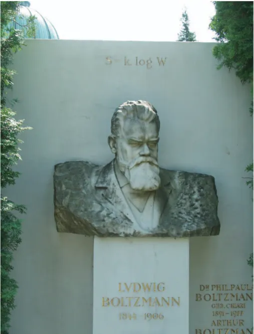
The solution to this paradox for classical systems was already provided by the pioneering work of Ludwig Boltzmann around the 1870s, who bridged the gap between the microscopic and macroscopic world by statistical arguments and by recognizing the importance of the initial condititions. His microscopic definition of entropy,S=kBlnW, relates the thermodynamic entropyS of a
macrostate with the number of microscopic statesW that are compatible with that given macroscopic state (which in turn is related to the probability of choosing that particular macroscopic state). The constantkB is added to get
the right units. Boltzmann’s explanation for the second law of thermodynam-ics is now a matter of comparing numbers of possible microscopic realizations. The entropy of a state where all the particles of the gas occupy one corner of a box is very small because there are not many microscopic ways to realize this configuration. Uniformly spreading the gas over the box increases the entropy because there are tremendously many more microscopic realizations of this macroscopic distribution. The calculation of entropy is thus reduced tocounting microscopic states and measuring phase space volumes. Together with the work of Planck, Einstein and Gibbs, statistical mechanics was born. From a reductionist perspective, statistical mechanics comes before thermo-dynamics, since it provides a microscopic description of a system. The ther-modynamic and macroscopic description can be recovered by appropriately reducing or coarse-graining the microscopic description. Furthermore, one has to go through the microscopic treatment of statistical mechanics to
under-stand and capture the corrections to thermodynamics in out of equilibrium situations. Following the work of Gibbs, the microscopic distribution
ρ(x) =e −βH(x)
Z
is introduced to describe systems in thermodynamic equilibrium. Here, the inverse temperature isβ= 1/kBT andH(x) is the energy of the system.
2. Beyond equilibrium: time enters the play
The theory of equilibrium statistical mechanics is well understood today in particular thanks to the aforementioned work of Gibbs, which provides a nat-ural framework to solve, at least in principle, any equilibrium problem. This does not mean that everything has been solved to the degree of satisfaction, as is the case for many complex equilibrium problems in the field of disordered systems. However, for the understanding of the world around us, it is vital to go to the much larger world of nonequilibrium situations: life is an excellent example of such a nonequilibrium system at work! No such general framework exists for systemsoutside equilibrium, which are typically systems driven by temperature differences or by different chemical potentials. Starting with the work of Onsager in 1930, a description of such systems was provided close to equilibrium, i.e., in a linear approximation. Also this framework breaks down when going far from equilibrium, for example when studying explosions (of which the most interesting occur in an astrophysical context), or when mod-elling living organisms. The more general problem is thus to find, if at all possible, a general framework of statistical mechanics, which is also able to cope with nonequilibrium situations. Of course, in this thesis only aspects of this ambitious project are highlighted.
One first remarks that the dynamics and time-dependence of the system play an important role for macroscopic nonequilibrium systems: temperature gra-dients or differences in chemical potentials induce heat and particle currents in the system. From the point of view of statistical mechanics, this gives rise to the question ofdynamically understanding the second law, which gives the arrow of time of the macroscopic world. After all, the second law of thermody-namics is an experimental fact of the macroscopic world, and any microscopic modelling of that world should reproduce this fact.
Again, it is the pioneering work of Ludwig Boltzmann that provides the first answers to this question. Boltzmann studied the mechanics of a dilute gas of hardcore particles. The macroscopic variable of interest was the one-particle velocity distributionf(~v, t) as a function of time. The first result of Boltzmann was to provide an autonomous evolution equation for this macroscopic variable:
∂f ∂t +~v·∇~f = ∂f ∂t coll ,
where the term on the right hand side describes the collisions between hardcore particles (which we will not discuss here). A second, and more surprising result was the so-calledH-theorem. Boltzmann defined theH-functional as
H(t) = Z
d~v f(~v, t) lnf(~v, t), and he was able to prove that
dH dt 60.
Boltzmann interpreted theH function as minus the entropy, and claimed that this mechanical derivation gave a proof of the second law of thermodynamics. The fact that an arrow of time arises from the time-reversal invariant micro-scopic collision laws already suggests that there are some subtleties in Boltz-mann’s derivation of the H-theorem. After a careful examination of Boltz-mann’s arguments, it turns out that the culprit is the assumption of molecular chaos, the so-calledStoßzahlansatz, which decorrelates the incoming and out-going directions of the velocities of two colliding particles in the dilute gas. However, one does not need this assumption to derive the Boltzmann equa-tion and the H-theorem: as Lanford showed in 1975 [59], it is sufficient to consider large systems with appropriate initial conditions and by looking at theproper timescales to recover the effective description of reality that is pro-vided by the Stoßzahlansatz and Boltzmann’s equation.
It turns out that for more general classical systems, beyond the scope of the Boltzmann equation, these three ingredients are indeed all that is needed to understand the emergence of the arrow of time in nonequilibrium systems. Boltzmann already realized this, and many afterwards have contributed to the better understanding of the increase of the Boltzmann entropyS =kBlnW.
We refer to the example of an analysis by Jaynes in 1965 [64]. When starting the system in a macroscopic state with a small W, i.e., if the initial state is sufficiently special so that few microscopic states correspond to it, then the time evolution of the system will almost certainly drive the microscopic state of the system to a region of high phase space weightW. This is again a simple matter of counting: by comparing phase space volumes, we immediately obtain that the system, during its dynamical excursion through the phase space, will almost certainly end up in a macroscopic state which corresponds to a huge number of corresponding microstates, i.e., with a high entropy S =kBlnW.
We will make this argument more precise in a later chapter, but again, it shows the importance of initial conditions, and of taking serious the fact that we are working with macroscopic systems. It is only for macroscopic systems with sizesN ∼1023 that the differences in phase space volumes W are huge
and lead to thermodynamically different values of the entropy. The system should also be studied at the appropriate time scale to avoid the Poincar´e re-currences of the microscopic Hamiltonian dynamics, which would violate the
H-theorem. However, for the macroscopic systems under consideration, these Poincar´e recurrences occur only at time scales of the order of 101023 seconds,
so we should not immediately worry about them.
The main conclusion is here that the second law of thermodynamics should not be viewed as an absolute truth, but rather as a result which is typically valid for large systems under appropriate initial conditions. The above ingredients and considerations work well in the context of classical systems. In this thesis, amongst other things, we attempt to generalize some of these arguments to closed quantum systems by closely studying the relation between entropy and irreversibility. To do this, we will study the quantity
R= ln Probρ[ω] Probσ[Θω]
,
as first introduced by Maes & Netoˇcn´y [80] in the context of classical systems. This quantity R relates the probabilities to observe a trajectory ω during a time-interval [0, τ], starting from an initial distribution ρ = ρ0, with the
probability of observing the time-reversed trajectory Θω, starting from the distribution σ. By choosing σ equal to the time-reversed version of ρτ, the
time-evolved measure of ρ0, the quantity R is a measure for the breaking of
time-reversal symmetry. The quest to undertake is to study the relation ofR with entropy,H-theorems and the second law of thermodynamics.
3. Fluctuation theorems for work and heat
Another popular line of research that goes beyond equilibrium situations is the study of so-called fluctuation theorems for dissipative quantities. The mo-tivation to study these fluctuations comes from the emerging research of nano-and biotechnology, where small devices have to operate nano-and function under “large” disturbances from the outside world. To give an idea of the energy scales involved, we refer to molecular motors which deliver work of the order of magnitude of a fewkBT’s while being subjected to thermal energy
fluctua-tions which are typically of that same order. Intuitively, this makes clear that we should study the average workwand the deviations thereof, which are of the order of magnitude ofwthemselves (the so-calledlarge deviations).
A fluctuation theorem is a statement about the symmetry properties of the probability distribution or probability density of an observableA. Generically, it is of the form
ln Prob[A=a]
Prob[A=−a] =Ca,
sometimes involving some kind of asymptotics for the system size or the ob-servation time and with C a constant. Such a relation was first observed in numerical experiments by Cohen, Evans and Morris [43], which led to the rig-orous formulation of a fluctuation theorem for the phase space contraction rate
by Gallavotti and Cohen [48, 49]. Within the context of chaotic dynamical sys-tems, the role of the observableAis played by the phase space contraction ratio
˙
S, which in turn is viewed in these references as the entropy production. This brings us back to the study of irreversibility. However, fluctuation relations for the entropy production give more information about how the typicality of the irreversibility, i.e., the increase of entropy, is attained. It does not only tell us that the probability Prob[ ˙S = λτ] for a positive entropy production
˙
S > 0 is much more likely than decreases in entropy, ˙S < 0, but also that the typical behaviour as discussed by Boltzmann is attained in an exponential fashion, in the Gallavotti-Cohen case asymptotically in the observation timeτ. Recently, van Zon and Cohen studied in a series of papers [121, 122, 123] a particle immersed in a fluid, and dragged by a harmonic potential at a constant velocity. Due to the collisions with the molecules in the fluid, the particle’s position, and hence also the derived quantities such as the work delivered on the particle and the heat dissipated by the particle to the environment, is a random variable. Van Zon and Cohen modelled the particle with Langevin dy-namics and concluded after an explicit calculation that the workWτ delivered
on the particle by an external agent satisfies, up to a multiplicative constant, the fluctuation theorem
ln Prob[Wτ =wτ] Prob[Wτ=−wτ]
=wτ, w >0.
This relation expresses that the probability for the unexpected event that the particle does work on the external agent, i.e.,Wτ <0, is exponentially damped
in the observation timeτ and thus becomes increasingly more unlikely. The first law of thermodynamics asserts that the heat Qτ differs from the
workWτ by the energy difference ∆U. One would expect that asymptotically
qτ = Qτ ≈ Wτ = wτ since ∆U/τ vanishes for large τ. Hence, it seems
tempting to extrapolate the fluctuation theorem for the work to an asymptotic fluctuation theorem for the heat:
lim τ→∞ 1 τ ln Prob[Qτ =qτ] Prob[Qτ =−qτ] =q.
Interestingly, this is not what happens: there is a nonzero probability that the particle stores the work Wτ done on it in the form of energy ∆U, thus
preventing ∆U/τ of going to zero asτ → ∞. This rare event gives rise to a correction of the fluctuation theorem. Again by explicit computations, van Zon and Cohen obtained that the heat satisfies the following extended fluctuation theorem: lim τ→∞ 1 τ ln Prob[Qτ =qτ] Prob[Qτ =−qτ] = q, forq∈[0, q[, q−(q−1)2/4, forq∈[q,3q[, 2, forq >3q,
where q is the mean heat dissipation per unit time. Here, we see that small fluctuations behave as one would expect in a fluctuation theorem. However the large fluctuations, which are more than 3q, are all equally damped in the observation timeτ, i.e., very large fluctuations in the heat are more likely than those in the work.
The case of the dragged harmonic potential is special in the sense that every-thing can be computed explicitly; this is possible because the work turns out to have a Gaussian distribution. Immediately, the question arises whether the correction to the fluctuation theorem discussed above is a peculiarity of the harmonic case, or whether it is more generally valid. Furthermore, it seems essential to understand why and under what circumstances such a correction for the heat can arise if one seriously wants to study heat dissipation, irre-versibility and entropy production. That is exactly what we have done in part of the present thesis.
4. A discussion on the results
Reversibility and irreversibility in the quantum formalism
The first result of this work concerns the relation between entropy and the breaking of time-reversal invariance in closed quantum systems. First, we have to define what we mean by a quantum trajectory of macroscopic states. The microscopic evolution, as determined by the Schr¨odinger equation, gives rise to an evolution at the level of macroscopic variables (the reduced or coarse-grained description). For example, we can study as a function of time the value of the total magnetization of a magnetic system as the macroscopic variable, while it changes under the microscopic evolution determined by a Hamiltonian. By performing measurements on the system at given times, we can write a se-quence of macroscopic states that the system has visited.
Using this notion of macroscopic trajectories, we can understand the relation between observing a particular macroscopic trajectoryωduring a time-interval [0, τ] and its time-reversed variant Θω. It turns out that also in a quantum mechanical description, the breaking of time-reversal symmetry can be related to the quantum Boltzmann entropy and Gibbs-von Neumann entropy. Roughly speaking, one has
ln Prob[ω]
Prob[Θω] =SB(ωτ)−SB(ω0),
whereSB(α) is the quantum Boltzmann entropy. An immediate consequence
is the positivity of the entropy production in closed quantum systems, un-dergoing an evolution which is interrupted by measurements to determine the macroscopic trajectory. From this, we recover statistical reversibility, a condi-tion similar to that of detailed balance, which in turn is known to express the
reversibility in standard stochastic models.
In standard textbook quantum mechanics, the underlying microscopic quan-tum dynamics is a combination of the reversible unitary time evolution as described by the Schr¨odinger equation, and the fundamentally irreversible col-lapse of the wave function. As such, there is no reversibility at the micro-scopic level since it is impossible to “unmeasure” or “decollapse” the system. However, as the result above shows, all this does not prevent the recovery of statistical reversibility.
On the other hand, the microscopic reversibility of the unitary evolution of quantum mechanics does not contradict the emergence of thermodynamic ir-reversibility. In a toy model, we study the magnetization ofN distinguishable spin-1/2 particles as a function of time, undergoing a standard unitary evo-lution. We are able to construct an irreversible, effective and autonomous dynamics at the level of the macroscopic variables, inspired by (but not using) Boltzmann’s assumption of molecular chaos or Stoßzahlansatz. We prove that for almost all conceivable realizations of our model, and for a large class of initial conditions, the unitary evolution converges to the effective dynamics as the system size grows. This leads to the conclusion that the reasons for ther-modynamic irreversibility are unchanged when going from the classical to the quantum world: it is again an interplay between the fact that we are working withlarge systems, using appropriateinitial conditions and by looking at the
proper timescales, in this case to avoid the quasi-periodicity of finite (but very large) quantum systems.
Fluctuation theorems for heat and work
In the mathematical context of a driven Langevin dynamics, we study a par-ticle under influence of a potential Ut that is changed according to a given
protocolγt. The observables of interest are the work performed on the particle
by the external agent that is modifying the potential, and the heat dissipated to the environment by the particle.
The conceptual framework is again that of looking at the breaking of time-reversal symmetry. A first result is the recovery of the so-called Crooks re-lation, which identifies the dissipation function and source of time-reversal symmetry breaking as thedissipative work Wdis=W−∆F. This dissipative
work is the total workW performed on the system, minus the reversible work ∆F, and as such it gives the energy lost through dissipation. The Crooks relation is valid for all potentialsUtand all protocolsγt.
It is known that there exist experimental set-ups in whichno fluctuation the-orem for the work is found. Therefore, an additional condition is needed to derive that fluctuation theorem from the Crooks relation, and when this condition is not verified, the fluctuation theorem should not hold. It turns
out that this additional condition is most conveniently expressed in terms of spatio-temporal symmetries of the potential and protocol: when the protocol is antisymmetric under time-reversal and the potential is symmetric under spa-tial reflections, or in case that the protocol is symmetric under time-reversal but then for any potential, we recover the fluctuation theorem for the work. Furthermore, we also find that the harmonic case of van Zon and Cohen is indeed special: the work always satisfies a fluctuation symmetry, regardless of spatio-temporal symmetries of the potential and protocol. Using numerical simulations, we are able to verify that the conditions for the existence of a fluctuation theorem are in fact optimal: from the moment they are not satis-fied, deviations from the fluctuation theorem can occur.
For the heat Q=W −∆U, we must understand under which circumstances the large deviations for ∆U give contributions of the order of the observation time τ to find back deviations from the fluctuation theorem that is valid for the work. We present a general argument based on the large deviation rate function of the work and the energy distribution ∆U. For general potentials, we recover the three regimes that were discussed by van Zon and Cohen. In our case, we can see clearly how the large deviations for the work are connected to the saturation of the fluctuation relation for large values of the heat per unit time q.
However, the main conclusion in the study of fluctuations is that again the framework of the time-reversal breaking is successful and unifies several re-cently proven results such as the Jarzynski equality, Crooks relation and fluc-tuation theorems in a broader picture.
5. Outline
This section briefly summarizes the content of each chapter and provides the grand master plan behind this thesis.
The first chapter contains a brief overview of some of the mathematical tools that are used in this work. We quickly review some aspects of classical Hamil-tonian mechanics and quantum mechanics. The emphasis there is on the dis-tinction between microscopic and macroscopic descriptions. Also some aspects of continuous diffusion processes for stochastic descriptions are discussed. It is not our goal to be very rigorous in the short overview that we present; the emphasis is on the conceptual framework, and when necessary, we will give references to other works for more details.
Chapter two presents a discussion of the concept of entropy, which will play a central role throughout this work. First, we go into detail on the defini-tions of entropy that exist in the literature: the reladefini-tions between the classical Clausius entropy, thermodynamic entropy, Boltzmann entropy, Shannon and Gibbs entropy will be discussed. We also give the quantum Boltzmann
en-tropy, the von Neumann and von Neumann-Gibbs enen-tropy, and summarize all entropies in the definition of relative entropy on the level of classical measures and density matrices. The chapter concludes with some words on the known relation between entropy and irreversibility in classical systems, and how we should understand the second law of thermodynamics. Again, it is not the intention to give a complete overview in this chapter, because much more can and should be said about the subtleties regarding the definition of entropy. On the other hand, the central role of entropy in the study of irreversibility forces us to review some results from the literature.
The third chapter proposes a relation between entropy and time-reversal sym-metry breaking in quantum systems. By looking at trajectories of macroscopic states, constructed by measuring at given times the macrostate of the system, we hope to find that the quantum Boltzmann entropy, which in some way measures the “quantum phase space volume”, measures the irreversible be-haviour of the quantum system. The concept of detailed balance, as known from stochastic models, will play an essential role in understanding the emer-gence of irreversibility in quantum systems.
After that, we turn in chapter four to the issues of the collapse of the wave func-tion and retrodicfunc-tion in quantum mechanics. The fundamental irreversibility of the collapse of the wave function seems to prevent microscopic reversibility of entering the quantum description. We will argue why the inability to undo measurements does not necessarily contradict the statistical reversibility at the level of trajectories, introduced in chapter three. To conclude that chapter, we also present the difficulties of retrodiction in quantum mechanics, and how this gives rise to seemingly paradoxical statements about simultaneous knowledge of noncommuting quantum observables.
Chapter five presents a simple quantum toy model which illustrates the con-cepts of the preceding two chapters. This model is a generalization of the Kac ring model, introduced in 1956 [66] to understand the reversibility paradox and the status of the Boltzmann H-theorem. The classical Kac model illus-trates in detail that there is no contradiction between macroscopic irreversible relaxation to equilibrium and the dynamical reversibility of the microscopic equations of motion. We lift this model to the quantum level and retrieve similar conclusions regarding irreversibility in quantum systems.
In chapter six, we turn back to classical systems and look at fluctuation re-lations for the work and heat in small systems. The goal is here to study Langevin systems which are more general than the dragged harmonic poten-tial of van Zon and Cohen. We provide a statement about the conditions for the existence of a fluctuation theorem for the work, and we can then under-stand when to expect corrections to a fluctuation theorem for the heat. This chapter also gives a review of some of the experimental tests of the known fluctuation theorems.
Finally, in chapter seven, we summarize the results by giving the conclusions of this work and we end by discussing some possible future extensions of this thesis.
Describing physical
systems
In the description of the reversible or the irreversible nature of physical phe-nomena, the scale will turn out to play a crucial role. In this chapter, we discuss some different scales of reality, and we explain how to attach a clas-sical or a quantum mechanical framework to the corresponding reality. We comment in a few lines on the history of decriptions of nature, to move along quickly to some of the mathematical frameworks that are known and used today.
1.1
Physical systems
1.1.1
Scene
Physics is about describing and unifying physical phenomena. That refers to the world around us, as composed of so-called physical objects. A remarkable definition of a physical object is read in Webster’s dictionary, which defines it as...
... an object having material existence: perceptible especially through the senses and subject to the laws of nature.
The reference to “material existence” is very much alive in contemporary and popular discussions, but goes in fact back to Aristotle, who lived around 350 B.C. That matter is composed of more elementary and universal build-ing blocks such as atoms was first conceived by the Greek atomists such as Democritus, around 400 B.C. At any rate, statistical physics talks about the emergence of the world around us out of those rawest material building blocks, and how it appears in mesoscopic or macroscopic conditions. Clearly, that rep-resents an enormous bridging of scales. Roughly speaking, we are interested in the global behaviour of about 1023particles as subject to the (microscopic)
logi-cally consistent statements which predict how one state of the object evolves into a new state.
1.1.2
Scales of objects and levels of description
Before going into the question on how to characterize a physical system, the level of detail of the description must be fixed.
The number of constituents of a physical object or system determines an im-portant scale, which in turn is related to the more visible scales such as time-, length- or energyscales. We restrict ourselves to two scales of objects in this thesis:
• microscopic objects
when less than approximately 104– 106elementary constituents are
in-volved in the composition of the object.
• macroscopic objects
when at least of the order of 1023 elementary constituents are involved
in the composition of the object.
Most objects that we can handle, feel and touch with our hands are typically composed of 1023atoms or molecules. The mesoscopic scale of approximately
106 to 1023 constituents will not be discussed here.
Though multiple levels of description exist, we shall restrict ourselves to two levels in this thesis:
• microscopic or complete description
where complete knowledge of all the 1023elementary constituents of the
physical object is required before the description is considered to be complete.
• macroscopic or reduced description
where only global properties concerning all or some of the elementary constituents of the physical object are required for the description to be considered complete.
From an everyday point of view, the macroscopic description is the most com-mon way of expressing the state of a physical object: it is sufficient to give the location, volume and temperature of a glass of water to have a good idea what the physical object under consideration looks and behaves like (water vapour, liquid water, ice).
Strictly speaking, there is no one-to-one mapping between the level of descrip-tion and the scale of the object under consideradescrip-tion. Obviously, microscopic descriptions work well for microscopic objects, and macroscopic descriptions for macroscopic objects. It is theoretically possible to give a microscopic (com-plete) description of a macroscopic object or to try to attach a macroscopic
description to a microscopic object. From a practical point of view, this is uncommon: a microscopic description of a macroscopic object requires the knowledge of about 1023 constituents and is currently beyond human and
computational capabilities.1 Attempting to connect macroscopic descriptions
to microscopic objects typically leads to interpretational problems of concepts like temperature, density or pressure.
1.1.3
Minimal requirements for a description of an object
For both microscopic and macroscopic descriptions, there are usually three ingredients that are used, for example, to make predictions about the physical object under consideration:
1. The initial state of the system which is the starting point for the description. Specifying the initial state also requires specification of the level of description (macroscopic or microscopic) and of the phase space. 2. The dynamics
which is required to specify how the initial state will evolve into another state of the system, and to determine which states are left invariant by the dynamics.
3. The physical properties of interest
or observables that we want to concentrate on.
The possible choices for these three ingredients depend on whether a classical or a quantum mechanical description is preferred. In the following sections, we will discuss both scenarios.
1.2
The description of classical systems
1.2.1
Microstates
The microscopic state x, or in short “microstate”, of a classical system is completely determined by specifying all the properties of each of the N con-stituents (which we will refer to as particles). We give two commonly used examples:
• To describe a mechanical system, the position ~qj ∈ R
3 and
momen-tum p~j ∈ R
3 of all particlesj ∈ {1, . . . , N} should be specified. The
microstate xdescribing the entire system is then given by x= (~q1, ~q2, . . . , ~qN, ~p1, ~p2, . . . , ~pN)∈R
6N.
We will usually group all positions and momenta together for a lighter notation and write x= (q, p).
1Nobody has succeeded up to today to give the full microscopic description of that
particular glass of water, and the author remains confident that nobody will for quite some time.
• To describe a magnetic system on a lattice Λ⊂Z
d, the (classical) spin~s j
or the intrinsic magnetic moment~µj=µB~sj (where the Bohr-magneton
µB is the proportionality constant) of each particle should be specified.
The microstatexis then given by
x= (~s1, ~s2, . . . , ~sj)∈SN,
whereSis the set of all possible (classical) spin values. For example, with Ising spins in one dimension, the possible spin values areS={−1,+1}. Remark that magnetism is a quantum phenomenon, but an excellent classical caricature can be obtained by the Ising “classical” spins. How to describe a full quantum spin is discussed in section 1.3.1.
In general, it is sufficient to provide the phase space Γ, which is the set of all possible microstatesx∈Γ and possibly subject to external constraints (such as particles in a box) and to internal conditions (such as fixing the energy). The specific interpretation of the microstate xis irrelevant for the following sections.
1.2.2
The microscopic dynamics
The phase space Γ provides us with one of the three ingredients to describe a system: states. To make things interesting, an evolution between these states must also be defined.
Hamiltonian dynamics
The Hamiltonian H(x, t) is a function from the phase space Γ into the real numbers R which, under standard conditions, represents the energy of the
system under consideration. For mechanical systems, a typical Hamiltonian is of the form H= N X j=1 ~ pj2 2m+ X i<j V(|~qj−~qi|),
whereV(~q) represents the potential energy at location~q. However, the Hamil-tonian is much more than the energy observable. It also plays the role of the generator of the time evolution ofN particles, which interact through the potentialV(~q). This time evolution is given by the Hamilton equations
dqi dt = ∂H ∂pi , dpi dt =− ∂H ∂qi , (1.1)
which describe how the initial microstatex0∈Γ of a mechanical system at an
level of the phase space, we can see the set of Hamilton equations as a flowft
which evolves the initial condition through ft: Γ→Γ :
x07→xt.
(1.2) The Hamiltonian flow is invertible: the inverseft−1exists, and one can go back
from a pointxt to the corresponding initial conditionx0 by applyingft−1 to
xt, see figure 1.1. x0 xt ft x0 xt ft -1
Figure 1.1: The inverseft−1 of the Hamiltonian flow ft allows to go back to the initial
statex0when applied to the final statext.
Consider a classical mechanical system going through a sequence of positions and momenta x0 = (q0, p0), . . . , xt = (qt, pt). That evolution solves
Hamil-ton’s equations of motion (1.1) for given forces, e.g., gravity. Upon playing the movie backwards, i.e., time reversed, we see the system evolving from the positionsqttoq0, but now with reversed momenta−ptto−p0.
In general, the time-reversed sequence (qt,−pt), . . . ,(q0,−p0) can or cannot be
a solution of the same equation of motion. For say free fall, the time-reversed sequence certainly solves the same Newton’s law of gravity; with friction or for the damped oscillator, that time-reversal symmetry is not present (but then we are no longer in the case of a Hamiltonian dynamics).
The Hamiltonian dynamics is always invariant2 under time-reversal, i.e., the
replacement of the timetby−t in the equations (1.1). Time-reversal changes the sign of the momentum
~ pj=
d~qj
dt ,
which represents the fact that we are playing the movie backwards. We for-mally define a time-reversal operationπ: Γ→Γ through3
π:x= (q, p)7→πx= (q,−p). (1.3) The time-reversibility of the Hamiltonian flow can then be formulated as
πftπ=ft−1.
2For systems under the influence of magnetic fields, also the direction of the magnetic
field should be inverted.
3For a Hamiltonian system in a magnetic field, the time-reversal operation becomes
In words: the inverseft−1of the Hamiltonian flow can be achieved by changing
the sign of the momenta inxt, and then applying the time-forward evolution
to πxt; to restore the proper initial state x0, the momenta must be reversed
once again (see also figure 1.2).
x0 xt ft -1 πxt ft ftπxt
Figure 1.2: Up to a change of momenta, the inverse evolutionft−1 can be attained by
applying the regular flowfttoπxt.
General dynamical systems
In general, e.g., for non-Hamiltonian or nonmechanical systems, the time evo-lution of the microscopic variables is of the form
dx
dt =F(x) (1.4)
and defines a flowft on the phase space Γ; thus, we can still writext=ftx0
as in the Hamiltonian case. However, the inverse of this general flowftdoes
not need to exist.
The notion of time-reversal invariance can be recovered for invertible flows.
Definition 1.2.1
An invertible dynamical flowftis calledtime-reversal invariantif and only
if there exists an involution π, withπ2=
1, such that
πftπ=ft−1. (1.5)
The involution π is referred to as the kinematic time-reversal or microscopic time-reversal.
If the phase space Γ has further structure, such as carrying a natural metric, then the involutionπis supposed to preserve that additional structure.
1.2.3
Distributions on phase space
In practical situations, it is often not well known what precise microscopic state the system is in: macroscopic systems require the knowledge of about 1023 positions and momenta! In those situations, it is often more convenient
Letρ(x) be a probability density on the phase space, in the sense that dρ(x) =ρ(x)dx
gives the probability for the system to be found in a microstate in the in-finitesimal phase space volume dx. The reference measure dx can be the Lebesgue/Liouville volume element or is derived from another natural metric. We consider here the classical statistical mechanics withdx=d~q1. . . d~pN. For
a given initial distribution ρ0(x) on the phase space, the Hamilton equations
(1.1) can be lifted to an evolution equation for the measure. Using the Liouville theorem
dρt
dt = 0, we obtain the Liouville equation
∂ρt ∂t + N X j=1 ∂ρt ∂qj ˙ qj+ ∂ρt ∂pj ˙ pj = 0,
which is usually4 written in terms of the Poisson bracket
{·,·}as ∂ρt ∂t =−{ρt, H}, {A, B} ≡ N X j=1 ∂A ∂qj ∂B ∂pj − ∂B ∂qj ∂A ∂pj . (1.6)
Because the Liouville equation implements the Hamiltonian flow (1.2), we have ρt(ftx) =ρ0(x). (1.7)
This relation expresses that keeping the initial distribution and evolving the phase points, is equivalent to evolving the distribution in time and keeping the phase points fixed.5
An important result in classical mechanics is that the Liouville volume
| · |:A7→ |A|= Z
A
dx, ∀A⊂Γ, (1.8)
with dx the Lebesgue measure (or in this context sometimes also called the Liouville measure), is preserved under the Hamiltonian flow (1.2)
|ftA|=|A|. (1.9)
4Another common way of writing the Liouville equation is
∂ρt
∂t =−Lρt,
whereL={·, H}is the Liouville operator or Liouvillian.
5In the quantum case, we would refer to this as the combination of the so-called
This is an expression of the fact that the Lebesgue measure dx, with proba-bility densityρL(x) = 1, is invariant under the Liouville evolution (1.6).
The Liouville measure and Liouville volume are important for Hamiltonian dynamics precisely because they give an unbiased and invariant way of com-paring the weight of sets in the phase space Γ. For a general dynamics (1.4), we will usually assume the existence of an invariant measure dρ, and define the phase space volumeρ(A) ofA⊂Γ as
ρ(·) :A7→ρ(A) = Z
A
dρ. (1.10)
1.2.4
Macrostates
Consider a classical, closed and isolated system of N particles. A complete description consists in specifying its microstate, which is a point x∈Γ in its phase space.
We wish to construct a reduced description which perhaps does not take into account all the details of the microscopic description. One obvious way to do that is to erase “information” from the level of description by specifying a map x∈Γ→f(x)∈ FwhereFis some metric space. The mapf is typically many-to-one and F is often some subspace ofR
n. A somewhat simpler picture of
that corresponds to dividing the phase space Γ into regionsM ⊂Γ, where, for example, on each subsetM the observablesf1(x). . . fm(x) take approximately
the same values6 for allx ∈ M. We write in such a case M = (f
1, . . . , fm)
wheref1=f1(x) for allx∈M. By doing this, each microstatexdetermines a
macrostateM(x) corresponding to that much coarser division of phase space: M :x→M(x).
Evidently, in the simplest case and to avoid ambiguities in the reduced de-scription, all the subsets Mα ⊂ Γ with (α = 1, . . . , n), should form a finite
partition of Γ, i.e., [
α
Mα= Γ, Mα∩Mα′ = 0 forα6=α′. (1.11) We group the macrostatesMαin the reduced phase space ˆΓ ={M1, . . . , Mn}.
Note that this partitioning could still depend on the number of particlesN in the system.
We emphasize that this reduced description involves macroscopic variables (in contrast with the partitions as used, e.g., in constructions of dynamical
6For observablesf which take values in a continuous interval [a, b]⊆
R, we should divide
the total interval [a, b] into smaller pieces [aj, bj]⊂[a, b] and assign a macrostateM(x) =Mj
entropies), such as position or velocity profiles and we denote by ρ(M) the corresponding phase space volume (1.8) or (1.10).
Sinceπis an involution, any phase space pointx∈Γ can be uniquely written as the kinematic time-reversal of another phase pointy∈Γ: x=πy. It is easy to find thisy, sincey=πxby the involution propertyπ2=
1. This one-to-one
mapping between a phase point x∈Γ and πxleads to the invariance of the Liouville volume under time-reversal for macroscopic states:
|πMα|=|Mα|. (1.12)
The microscopic flowft:x0 7→xt, which can be Hamiltonian as in equation
(1.2), implies a dynamics at the level of the reduced phase space ˆΓ, where now M0 ≡ M(x0) 7→ M(xt). A priori, there is no reason to exclude that
the image ft(M0) of a macrostateM0⊂Γ overlaps with several macrostates,
i.e., that there exist multipleMα∈Γ for whichˆ ft(M0)∪Mα6=∅, see figure 1.3.
Γ
M
0f
t(
M
0)
f
tFigure 1.3:The phase space Γ is divided into smaller cellsM∈ˆΓ that form the macroscopic states. Usually, this division is inspired by a set of macroscopic observables taking constant values on each cellM. The microscopic flowft (which does not need to be Hamiltonian)
evolves one macrostate M0 into its imageft(M0), which a priori can overlap with several
macrostatesMα∈Γ.ˆ
However, it can happen that the dynamics on the level of the macrostates is
autonomous, which means that from (only) knowing the macrostate M0 at
some given time, we also know the macrostateMtat a later time. Typically,
the separation between the microscopic and macroscopic world manifests itself in the form of hydrodynamic or thermodynamic limit, where the number of particlesN → ∞. It is only in this limit that we expect that the macroscopic degrees of freedom detach from the microscopic world and that autonomy is
established. In that case, the imageft(M0) of the macrostateM0is obviously
concentrated in the macrostateMt, and hence, if only formally,
ft(M0)⊂Mt ⇒ ρ ft(M0)6ρ Mt,
where again,ρis the invariant measure for the flowft.
Even though autonomy seems like a very serious restriction on the level of the microscopic dynamics, it is what we expect to find in the macroscopic world, at least for a “good choice” of macroscopic observables. For example, Newton’s equations of motion for macroscopic objects subject to friction, the Navier-Stokes equations for fluid dynamics or the Boltzmann equation for dilute gases, are all for a large part independent of the details of the microscopic world. Yet, they successfully give an autonomous, macroscopic description of reality.
1.3
The description of quantum systems
1.3.1
Microstates
In quantum mechanics, the full description of a system is no longer given by all the positions and momenta of all particles, but by the wavefunction |ψi
from a Hilbert space H, i.e., a complete, normed vector space with the norm induced by a scalar product. It has been argued that this description does not always provide the full picture, but we will not consider that question here. We will usually assume thatHis finite dimensional.
Single particle Hilbert space
The precise form of the Hilbert space depends on the degrees of freedom of the quantum system that are taken into account. The spatial degrees of free-dom are described by a normalized, square integrable wave functionψ(q, t) in L2(
R
3, dq). Following Born’s statistical interpretation of the wave function,
we interpret
|ψ(q, t)|2dq
as the probability for finding the particle in an infinitesimal volume [q, q+dq] at the timet. Obviously,
Z
R
3|
ψ(q, t)|2dq= 1
is now the normalization of the probability distribution.
Since Pauli’s theoretical work and as, e.g., manifested in the Stern-Gerlach ex-periment, a quantum description also sometimes involves an intrinsic quantity known as spin. For our purposes, it is sufficient to say that the quantum spin is described by a normalized vector~s∈C
with the most relevant case ofj= 1/2, so the Hilbert space isC
2.
The total wave function for the system is then given by
|ψi=ψ(q, t)⊗~s∈ H, H=L2(R
3, dq) ⊗C
2j+1.
To determine the expectation values of position and momentum, the corre-sponding operators must be defined. In the position representation, the mo-mentum operator is given by
pm=−i~ ∂
∂qm, m∈ {x, y, z}. (1.13)
The operators that give the three components of a spin 1/2 particle are, up to a constant~/2, given by the Pauli matrices:
σx= 0 1 1 0 , σy = 0 −i i 0 , σz= 1 0 0 −1 .
In general, we write A for the algebra of observables working on the single particle Hilbert spaceH.
Multiple particles
For quantum systems composed ofN distinguishable particles or components, the Hilbert space HN that contains the wave functions|ψithat describe the
entire system, is built up from the single particle Hilbert space H =Hj for
thejth particle: HN = N O j=1 Hj.
We writeAN for the algebra of observables working onHN.
1.3.2
Microscopic dynamics
The Schr¨odinger equation of quantum mechanics
The Hamiltonian H is an operator on the Hilbert space HN and represents
in some way the energy of the system under consideration. In the standard set-up and Schr¨odinger representation, a typical Hamiltonian is of the form
H= N X j=1 −~ 2 2m ∂2 ∂~qj2 +X i<j V(|~qj−~qi|),
where ~pj = −i~∂/∂~qj is the momentum operator and V(q) is the potential
energy operator. The Hamiltonian generates the dynamics as given by the Schr¨odinger equation:
i~∂
with the formal solution |ψti=Ut|ψ0i, Ut= exp −itH~ . (1.15)
The unitary evolution Ut implements the evolution flow on the algebra of
observablesAas
At=Ut†AUt, (1.16)
where† represents the operation of Hermitian conjugation andA∈ A.
Time-reversal invariance of the Schr¨odinger evolution
One of the most visible formal differences between the Schr¨odinger equation and Newton’s law is that the Schr¨odinger equation (1.14) is first order in time while Newton’s F = ma is second order.7 Clearly then, the fact that |ψti=ψ(q, t) is a solution of the Schr¨odinger equation (1.14) does not imply
that|ψ−ti=ψ(q,−t) is also a solution, as was the case for Newton’s or
Hamil-ton’s equations (1.1). In thatvery strict sense, Schr¨odinger’s equation is not time-reversal invariant.
We hasten to give the standard response, that one should also complex conju-gate: |ψtiis a solution if and only if|ψt⋆iis a solution. One argument comes
from the representation of the momentum (1.13), where the complex conjuga-tion switches the sign of the momentum. One could reply to that by noting that there is noa priori reason that the momentum should change sign under time-reversal: after all, in equation (1.13), there is only a spatial (and no time-) derivative. Furthermore, it is not clear in general how to realize experimen-tally a complex conjugation on the wave function of a system. Nevertheless, the more fruitful response is to complement time-reversal with a certain oper-ation on wave functions much in the spirit of the kinematic reversibility (1.5) as we will now explain.
One of the advantages of the abstraction around the definition of kinematic reversibility (1.5) is that it also applies to the free evolution of the quan-tum formalism, i.e., the evolution on wave functions as given by the stan-dard Schr¨odinger equation (1.14). Following the proposal of Wigner [128], the recipe for time-reversal is to apply complex conjugation. More generally, the transformationπ of above is now an antilinear involution on the Hilbert space, π2 =
1. We get time-reversal symmetry when thatπ commutes with
the quantum HamiltonianH. Since the Schr¨odinger evolution is given by the unitary (1.15), equation (1.5) can now be written as
πUtπ=Ut†=Ut−1, (1.17)
7One could argue that Schr¨odinger’s equation consists of two first order equations (since
ψ is complex), very much analogous to Hamilton’s equations of classical mechanics. This does not diminish the fact that there is still an essential difference.
where through the complex conjugation of the momentum (1.13), we still have π(q, p) = (q,−p), albeit through a different mechanism than in classical me-chanics.
We conclude that not only the (classical) Hamiltonian equations, but also the Schr¨odinger equation8are effectively invariant under dynamical time-reversal:
for the free quantum flow, future and past are mere conventions and can be described by the same laws. Once the measurement procedure of collapsing the wave function enters, we no longer have a free quantum evolution. Then, things get more complicated as we will discuss in chapter 4.
The von Neumann measurement postulate
To give the full time evolution of a quantum system, the Schr¨odinger equation (1.14) is usually supplemented with the collapse of the wave function. Von Neumann, known for his rigorous mathematical approach to the foundations of quantum mechanics, argues that in order for quantum mechanics to be a fundamental theory, it must also be able to describe the act of measurement [125, p418]:
First, it is inherently entirely correct that the measurement or the related process of the subjective perception is a new entity relative to the physical environment and is not reducible to the latter. Indeed, subjective perception leads us into the intellectual inner life of the individual, which is extra-observational by its very nature[...] Nevertheless, it is a fundamental requirement of the scientific viewpoint – the so-called principle of the psycho-physical parallelism – that it must be possible so to describe the extra-physical process of the subjective perception as if it were in reality in the physical world – i.e., to assign to its parts equiva-lent physical processes in the objective environment, in ordinary space.
– John von Neumann
The measurement in quantum mechanics collapses the wave function to the eigenstate of the observable being measured, corresponding to the eigenvalue that was measured. Write the spectral decomposition of an observableA∈ A as A= n X j=1 ajPaj, where aj ∈ R are the eigenvalues of A and Pa
j = P
2
aj is the projector on the eigenspace corresponding toaj. Von Neumann postulates that when the
measurement of the observableAon the wave function|ψiyields the eigenvalue
8Or, for that matter, Dirac’s equation. We do not wish to speak about time-symmetry
aj as an outcome, then the after-measurement wave function |ψ′iis given by, see [24]: |ψ′i= Paj|ψi p hψ|Paj|ψi . (1.18)
The probability to measure the eigenvalueaj as the outcome is postulated to
be
Prob(A=aj) =hψ|Paj|ψi. (1.19) This shows that the measurement is the point where stochasticity enters into the quantum dynamics: at the point of measurement, the system randomly chooses one of the eigenstates of the measured observableA to collapse to, of course verifying the probability distribution Prob(A=aj).
1.3.3
Macrostates
As in the classical case, we would like to split the Hilbert space into smaller parts Mα ⊂ H corresponding somehow to the joint eigenspaces of a set of
macroscopic observables (A1, . . . , Am). The variables defining the macrostate
are not different from that in the classical situation. For example, they specify (again to some appropriate accuracy) the particle number and the momentum profiles by associating numbers to a family of macroscopically small but mi-croscopically large regions of the volume occupied by the system.
However, this is not trivial: in the quantum case, the observables which are used for the division of the Hilbert space might not commute. Therefore, the concept of joint eigenspace is rather suspect. One says that it is not possible to measure noncommuting observables simultaneously. This makes it hard from an experimental viewpoint to determine if a wave function|ψishould belong to a certain Mα ⊂ H. In this context, von Neumann [125, p.402] remarked
that:
Now it is a fundamental fact with macroscopic measurements that everything which is measurable at all, is also simultaneously measurable, i.e., that all questions which can be answered sepa-rately can also be answered simultaneously.
– John von Neumann
From this we conclude that the problem should disappear in the thermody-namic limit. We refer the interested reader to reference [32] for an extensive discussion.
This problem vanishes, or is expected to vanish, for very large systems, for whichN → ∞. For intensive observables of the form
AN = 1 N N X j=1 Aj,
whereAj works at a small number of sites, we find [AN, BN] =O 1 N →0.
Therefore, for large systems, we can safely assume that the macrostate is given in terms of the values of a set of macroscopic observables represented by commuting operators. We refer to reference [32] for more details on the construction of the microcanonical quantum ensemble.
Then, the macroscopic partition in the classical case (1.11) is replaced by the orthogonal decomposition of theN-particle Hilbert spaceH:
H=M
α
Hα (1.20)
into linear subspaces. These linear subspaces can be found common to all the commuting operators that have been chosen as the macroscopic variables for the partitioning. The macrovariables are represented by the projectionsPαon
the respectiveHα, where
PαPβ=δα,βPα, and
X
α
Pα=1.
We writedα for the dimension ofHα,Pαdα=d= dim(H); the quantitydα
is the analogue of the Liouville volume|M|(1.8) of the classical case.
We also assume that the macrostatesα, corresponding to the decomposition of the finite-dimensional Hilbert space H(1.20) are mapped into each other via the involutionπ, i.e.,
πPαπ=Pα′ ≡P
πα (1.21)
for some α′, for eachαand we write πα=α′. Remark that this implies dπα=dα,
just like in the classical case (1.12).
1.3.4
Pure states and statistical mixtures
Up to now, we have discussed quantum systems for which the microscopic state|ψiof the entire system was well known. In many practical situations, this is of course not the case: if we are given the temperature of the system, we have knowledge about the average energy of all the particles, and with some luck we can derive more information about the actual distribution of energies of the system.
The question is now how to incorporate our incomplete knowledge of the mi-croscopic state of the system into the quantum formalism. A natural way to do this, is by using probability theory and introducing statistical mixtures of quantum states.
The density matrix
Suppose that the states |ψki form a complete, orthonormal set with9 k ∈ {1, . . . , d}. Write Pk = |ψki hψk| the projector on the state |ψki, then the
projectorsPk form an orthonormal decomposition of unity: d
X
k=1
Pk=1, PkPm=δkmPk.
We are given a probability distributionpk on the states|ψki,Pkpk= 1. If we
know that the system is in state|ψkiwith a probabilitypk, then the density
matrixρ, describing this statistical mixture of quantum states, is defined as ρ= d X k=1 pkPk = d X k=1 pk|ψki hψk|. (1.22)
Due to the lack of exact information about the microscopic state of the system, we simply refer toρas the state of the quantum system under consideration. A stateρis calleda pure state if the probability distributionpk concentrates
on one value ofk, i.e.,
ρ=|ψki hψk|.
We find that for pure states,ρ2=ρ. It can be proven that this is a necessary
and sufficient condition for a state to be pure. This also illustrates how pro-jection operators can be used to describe systems for which the expectation value of a given observable is known.
It is important to emphasize that we now have two different sources of stochas-ticity in the quantum description:
• First of all, there is the probability in the initial distribution of the sys-tem. This is the stochasticity that enters through the probability distri-butionpkof above. This expresses our ignorance of the exact microscopic
state: the quantum system is in the pure state|ψ1iwith probabilityp1
or it is in the pure state |ψ2i with probabilityp2 or . . . orit is in the
pure state|ψdiwith probabilitypd.
• Secondly, there is the fundamental probabilistic aspect of quantum me-chanics which is hidden in the collapse postulate: a wave function |ψi can be a superposition of several eigenstates of a given observable, i.e.,
|ψi=
d
X
k=1
ck|ψki.
9We will assume that there is no degeneracy in the eigenvalues of the eigenstates|ψ
ki,
so the indexkruns from 1 tod, the dimension of the Hilbert space. In case of degeneracy, this upper index should be appropriately adjusted in all the formulas.
This means that the system is in the pure state|ψ1iwith a probability |c1|2 to find it there when measuredand that the system is in the pure
state |ψ2i and . . . and in the pure state |ψdi. Related to this is the
probabilistic nature of the measurement, which was discussed at the end of section 1.3.2.
Properties of the density matrix
We quickly review the most important properties of the density matrix. The density matrix is a positive (and thus Hermitian) operator with trace one:
ρ >0, Tr[ρ] = 1.
The expectation value of an observableAin the state described by the density matrixρis given by hAiρ= Tr[ρA] = d X k=1 pkhψk|A|ψki. (1.23)
In other words,hAiρ is thepk-weighted average of the expectation values ofA
in each pure state|ψkiof the mixtureρ.
The time evolution as described by the Schr¨odinger equation can be lifted to the level of density matrices. The resulting equation is the quantum analogue of the Liouville equation (1.6):
dρt
dt =− i ~[H, ρt],
whereHis the Hamiltonian describing the system. The formal solution of this equation is given by ρt= exp −~i[H,·] ρ0,
which is very similar to equation (1.15) for pure states. Using the notationUt
for the unitary evolution (1.15), we get
ρt=Utρ0Ut†, (1.24)
which should be compared to the evolution (1.16) for observables.
For composite quantum systems, the partial trace can be used to compute the marginal density matrices for a component of the system. For a Hilbert space
H=H1⊗H2, the partial trace operation for the first componentH1is defined
as
Tr1[A⊗B] =ATr[1⊗B]
which can be linearly extended to general operators on H. At the level of density matrices, we write
ρj= Trjρ (1.25)
for the marginal at componentjof the density matrixρin some decomposition
Density matrices and measurements
Write the spectral decomposition of an observableAas A=
d
X
j=1
ajPaj,
where thePaj are orthogonal projectors. Given a general density matrixρ, we can takeA=Paj in the expectation value (1.23) to find the generalization of equation (1.19): Probρ(A=aj)≡Tr[Pajρ] = d X k=1 pkhψk|Paj|ψki, (1.26) which gives the probability for the valueaj to be measured when the state of
the system is given byρ.
Whenever a measurement occurs, the collapse of the wave function is imple-mented by a projection corresponding to the after-measurement eigenspace, see equation (1.18). When the measurement on a system described by density matrixρhas the specific outcomeaj, then von Neumann [125, p.351] teaches
that the corresponding after-measurement density matrix is given by ρ′= PajρPaj
Tr[PajρPaj]
, (1.27)
i.e., we sandwich the original density matrix between the projector correspond-ing to the outcome and normalize this new density matrix. We can also mea-sure the system without looking at the outcome: in this case, we don’t collapse onto one particular realization of the observableA:
ρ′=
d
X
j=1
PajρPaj (1.28) We skip the discussion of nonideal or other than von Neumann measure-ments, where the projectors are replaced by positive operator valued measures (POVM).
1.4
The description of stochastic systems
At many instances, our understanding of physical phenomena involves sta-tistical considerations. Even when God does not play dice and also for the description of the classical world, depending on the scale of the phenomena, stochastic dynamics enter. They can be the result of pure modelling or they ap-pear as an effective or reduced dynamics. Classical examples are the Langevin description of Brownian motion, the Onsager-Machlup description of fluctu-ating hydrodynamics and the stochastically driven Navier-Stokes equation for


![Figure 2.6: The Penrose [94] representation of how well-chosen the initial condition of the universe is](https://thumb-us.123doks.com/thumbv2/123dok_us/9540515.2438412/93.680.178.518.95.317/figure-penrose-representation-chosen-initial-condition-universe.webp)

