Multivariate Poisson Distributions Associated with Boolean Models

(1)

U n i v e r s i t ä t A u g s b u r g

Institut für

Mathematik

Christian Br¨

au, Lothar Heinrich

(2)

Impressum:

Herausgeber: Institut für Mathematik Universität Augsburg 86135 Augsburg http://www.math.uni-augsburg.de/de/forschung/preprints.html ViSdP: Lothar Heinrich Institut für Mathematik Universität Augsburg 86135 Augsburg

(3)

Multivariate Poisson Distributions Associated

with Boolean Models

Christian Bräu and Lothar Heinrich

1

Abstract

We consider ad−dimensional Boolean model Ξ = (Ξ1+X1)∪(Ξ2+X2)∪ · · · generated by a Poisson point process{Xi, i≥1}with intensity measure Λ and a sequence{Ξi, i≥1}

of independent copies of some random compact set Ξ0. Given compact sets K1, ..., K`,

we show that the discrete random vector (N(K1), . . . , N(K`)), where N(Kj) equals the

number of shifted sets Ξi+XihittingKj, obeys a`−variate Poisson distribution with 2`−1

parameters. We obtain explicit formulae for all these parameters which can be estimated consistently from an observation of the union set Ξ in some unboundedly expanding window

Wn (asn→ ∞) provided that the Boolean model is stationary. Some of these results can

be extended to unions of Poissonk−cylinders for 1≤k < d and more general set-valued functionals of independently marked Poisson processes.

Keywords : _{random closed sets, independently marked Poisson process,} gen-erating functional, multivariate probability gengen-erating function, higher-order covariances, empirical volume fraction

AMS 2010 MSC :Primary: 60D05, 60E05; Secondary: 60E10, 62F10

1 Introduction and preliminaries

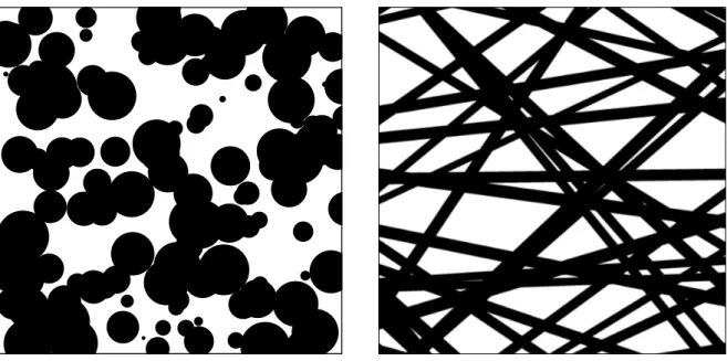
The Boolean model (briefly BM; also known as Poisson grain or Poisson blob model) is one of the best studied and most frequently used models to describe two-phase systems of random sets which decompose thed-dimensional Euclidean space _Rd into a vacant region (white) and a region consisting of irregularly shaped clumps (black), see Fig.1. This clumping structure is generated by unions of completely randomly distributed independent random compact sets,

1

Corresponding author: Institute of Mathematics, Augsburg University, 86135 Augsburg, Germany E-mail: [email protected]

(4)

Figure 1: Realization of a 2D-Boolean model with discs

Figure 2: Realization of a 2D-Poisson strip process

see e.g. [12], [4], [13],[16],[2] for more details. To be precise, we first recall the definition of a (not necessarily stationary) BM Ξ = Ξ_Λ_,Q as countable union set

Ξ_Λ_,Q= [ i≥1

( Ξi+Xi) (1.1)

of independent copies Ξ₁,Ξ₂, . . .of a generic random compact set Ξ₀ (calledtypical grain) with distributionQ(on the Borelσ-algebraB(Kd_{), where}_Kd_{denotes the metric space of non-empty} compact sets in _Rd equipped with the Hausdorff metric), where the Ξi’s are independently shifted by the atoms of the Poisson point process Π_Λ =P

i≥1δXi with locally finite intensity

measure Λ on the Borelσ-algebra B(_Rd). For notational ease, each atom of the locally finite random counting measure Π_Λ occurs in the sum P

i≥1 resp. in the union

S

i≥1 according to

its multiplicity, where Π_Λ has multiple atoms iff Λ has atoms, see [16], p. 59. By definition of Π_Λ, the random numbers Π_Λ(B1), . . . ,ΠΛ(B`) are mutually independent if the bounded sets

B1, . . . , B` ∈ B(Rd) are pairwise disjoint and ΠΛ(Bj) is Poisson distributed with mean Λ(Bj) forj= 1, . . . , `. The stationarity of Π_Λand thus the stationarity of the BM (1.1) is equivalent with the shift-invariance of the intensity measure Λ and this in turn means that Λ(·) =λ| · |d with some constantλ >0 (called intensity of the BM) and Lebesgue measure | · |_d on B(_Rd_). In what follows, Ξλ_Q will denote a stationary BM with intensity λ >0.

The random union set Ξ_Λ_,Q defined by (1.1) over some probability space [Ω,F,P] (which always exists) need not to be closed P-a.s., see e.g. [7] for counterexamples. The (P-a.s.)

(5)

closedness of the BM (1.1) is guaranteed iff, for anyr >0 ,

0<

Z

Rd

Q({K ∈ Kd: (K+x)∩B_rd6=∅}) Λ(dx) =EΛ Bd_r⊕(−Ξ0)<∞, (1.2)

where B_rd := {x ∈ _Rd _:_k_x_{k ≤} _r_} _and _A_⊕_B _:= _{_a₊_b _:_a _∈ _{A, b} _∈ _B_}_{, see [12] and [5] as} special case of closedness conditions for general grain-germ models.

Under condition (1.2) the random variable

N(K) = #{i≥1 :K∩(Ξ_i+Xi)6=∅}, (1.3)

taking values in _Z₊ = {0,1,2, . . .} is (as consequence of our model assumptions) Poisson distributed with finite mean EΛ K ⊕(−Ξ0) > 0 for each K ∈ Kd. In this paper we are

interested in the distribution of the _Z`₊-valued random vector N(K1), . . . , N(K`) for fixed pairwise different, compact sets K1, . . . , K` inRd and any`≥2. Obviously, the components

N(Ki) are correlated random variables unless Ξ0 is bounded and theKi’s are specially chosen. In [1] the special case of two distinct points x, y ∈ _Rd _{has been treated by a rather lengthy} explicit computation of the probabilitiesP(N({x}) =i, N({y}) =j) fori, j= 0,1, . . .. In Sect. 2 we extend this result in two ways, namely, we consider more than two pointsx1, . . . , x` and can even replace thexi’s by compact sets Ki. To avoid the awfully long computation of the joint probabilities of {N(Ki) = ni}, i= 1, . . . , `, we derive instead in Theorem 2.1 the shape of the probability generating function (short: PGF)

E zN(K1) 1 · · ·z N(K`) ` = X n1,...,n`≥0 zn1 1 · · ·z n` ` P(N(K1) =n1, . . . , N(K`) =n`) (1.4) forz1, . . . , z` ∈C1 satisfying max1≤i≤`|zi| ≤1.

It turns out that N(K1), . . . , N(K`)

possesses an `-variate Poisson distribution. Since there exist different multivariate extensions of the Poisson distribution, see e.g. [9], we recall the definition of that`-variate Poisson distribution which seems to be most meaningful not only in our situation. A random vector (N1, . . . , N`) with values in Z`+ is said to be`-variate Poisson

distributed if its PGFg(z1, . . . , z`) =E zN1 1 · · ·z N` `

possesses the form

g(z1, . . . , z`) := exp n _X ∅6=J⊆L µJ Y j∈J (zj−1) o = expnγ∅+ X ∅6=J⊆L γJ Y j∈J zj o (1.5)

for allz1, . . . , z` ∈C1 with positive expectationsµi =ENi and further 2`−1−` parameters

(6)

cumulant of the subvector (Nj)j∈J which have to satisfy the consistency conditions γ∅:= X ∅6=J⊆L (−1)#JµJ <0 and γI:= X I⊆J⊆L (−1)#(J\I)µJ ≥0 for ∅ 6=I ⊆L . (1.6)

The conditions (1.6) are necessary (and sufficient) for a non-degenerate `-variate Poisson distribution since (1.5) implies the relations ₍_∂z∂#I

i)i∈I logg(z1, . . . , z`) ≥ 0 for I ⊆ L and all

z1, . . . , z` ∈ [0,1] and γ∅ = −P∅6=I⊆LγI. Various structural properties of this multivari-ate Poisson distribution are known : (i) its existence as limit of multivarimultivari-ate binomial dis-tributions, see [10], (ii) its characterization by recurrence relations of the density functions

P(N1 =n1, . . . , N` =n`), see [11] and (iii) it is the only infinitely divisible distribution which is marginally Poisson, see [3] and [9]. It is noteworthy to mention thatµij =Cov(Ni, Nj) = 0 for i 6= j implies independence of the components Ni and Nj. On the other hand, µij = 0 for all pairs i, j ∈ L , i6= j ,#L ≥ 3, does not necessarily imply neither µL = 0 nor mutual independence of the components N1, . . . , N`. The rest of this paper is organized as follows: In the next Sect. 2 we formulate and prove the announced main result for BM’s. In Sect. 3 we shall discuss the parameters in case of a stationary BM and derive strongly consistent estimators for all parameters occurring in the PGF (2.7) based on an single observation of the union set (1.1) in an unboundedly increasing sampling window Wn. In the final Sect. 4 we extend Theorem 2.1 to other random set models driven by independently marked Poisson processes.

2 Main result

Theorem 2.1. Let Ξ_Λ_,Q be a BM as defined by (1.1) satisfying (1.2). Then the PGF of the random vector N(K1), . . . , N(K`)with components defined by(1.3)for fixedK1, . . . , K` ∈ Kd

such thatmin₁≤i≤`EΛ(Ki⊕(−Ξ0))>0 takes the form

EhzN(K1) 1 · · ·z N(K`) ` i = expn X ∅6=J⊆L EΛ \ j∈J (Kj⊕(−Ξ0) ) Y j∈J (zj −1) o , (2.7)

where the sum P

∅6=J⊆L runs over all 2`−1 non-empty (unordered) subsets J of L. In other

words, N(K1), . . . , N(K`)

possesses an `-variate Poisson distribution with parameters

µJ =µΛ,Q(KJ) :=EΛ \

j∈J

(Kj ⊕(−Ξ0)) for ∅ 6=J ⊆L (2.8)

and the consistency relations (1.6) are fulfilled with γJ =γΛ,Q(KJ) defined by

γΛ,Q(KJ) :=EΛ \ j∈J (Kj⊕(−Ξ0) )−EΛ \ j∈J (Kj⊕(−Ξ0) )∩ [ j∈L\J (Kj⊕(−Ξ0)) (2.9)

(7)

for ∅ ⊆J ⊆L

Proof. For each copy Ξi of the typical grain Ξ0 and any compact set K6=∅, it is evident that

K∩(Ξ_i+Xi)6=∅ iff Xi∈K⊕(−Ξi).

Therefore, using the indicator function1B(x) (= 1 forx∈B and = 0 otherwise) we may write

N(K) as sum N(K) = # i≥1 :K∩(Ξ_i+Xi)6=∅ = X i≥1 1K⊕(−Ξi)(Xi).

Hence, forz1, . . . , z`∈C1 we may express the PGF of N(K1), . . . , N(K`)as follows:

EhzN(K1) 1 · · ·z N(K`) ` i =Eh Y i≥1 z1K1⊕(−Ξi)(Xi) 1 · · ·z 1_K`⊕(−Ξ_i)(Xi) ` i .

Next, we make use of the probability generating functionalGΛ,Q[v] =E Q

i≥1v(Xi,Ξi)of an independently marked Poisson process Π_Λ_,Q=P

i≥1δ[Xi,Ξi]onR

d_{× K}d_{with intensity measure} Λ and mark distributionQ. GΛ,Q[v] possesses a comparatively simple shape, see e.g. [16] (p. 65) or [2], namely, G_Λ,Q[v] = exp Z Rd Z Kd v(x, K)−1 Q(dK) Λ(dx) (2.10)

for any Borel-measurable function v|_Rd_{× K}d_−→_C1 _satisfying

R Rd

R

Kd|v(x, K)−1|Q(dK) Λ(dx)<∞ .

In the particular case v(x, K) =Q`_j₌₁z_j1Kj⊕(−K)(x) the latter condition is an immediate conse-quence of (1.2). By applying the obvious identities z1B(x)= 1 +1B(x)(z−1) and

Y j∈L (1 +aj) = 1 + X ∅6=J⊆L Y j∈J ai (2.11)

for any a1, . . . , a` ∈ C, where the sum P∅6=I⊆L runs over all non-empty index sets I ⊆

{1, . . . , `}, we can express v(x, K)−1 as follows:

v(x, K)−1 = Y j∈L 1 +1Kj⊕(−K)(x)(zj −1) −1 = X ∅6=I⊆L Y i∈I (zi−1)1Ki⊕(−K)(x) .

(8)

Fubini’s theorem we arrive at EhzN(K1) 1 · · ·z N(K`) ` i = expn X ∅6=J⊆L Y j∈J (zj−1) Z Rd Z Kd Y j∈J 1Ki⊕(−K)(x)Q(dK) Λ(dx) o = expn X ∅6=J⊆L Y j∈J (zj −1) Z Rd Z Kd 1T j∈J (Kj⊕(−K))(x)Q(dK) Λ(dx) o = expn X ∅6=J⊆L Y j∈J (zj −1)EΛ \ j∈J (Kj⊕(−Ξ0) ) o .

The last line provides the asserted shape of the PGF (2.7).

To accomplish the proof of Theorem 2.1 we check the conditions (1.6) forµJ given in (2.8). For notational ease we putK_i0 :=Ki⊕(−Ξ0) for i= 1, . . . , `and ν(·) =EΛ(·). Applying the

inclusion-exclusion formula

ν(A∩ ∪_j_∈_L_\_IAj) = X

∅6=J⊆L\I

(−1)#J−1ν(A∩ ∩_j∈JAj)

(being valid for any additive set-functionν) yields

γΛ,Q(KI) = X I⊆J⊆L (−1)#(J\I)ν(\ j∈J K_j0) =ν \ i∈I K_i0 + X ∅6=J⊆L\I (−1)#Jν \ i∈I K_i0∩ \ j∈J K_j0 =ν \ i∈I K_i0 −ν \ i∈I K_i0∩ [ j∈L\I K_j0 ≥0 for ∅ 6=I ⊆L

and, sinceEΛ(Ki⊕(−Ξ0))>0 fori= 1, . . . , `,

γΛ,Q(K∅) = X ∅6=J⊆L (−1)#Jν(\ j∈J K_j0) =−ν [ j∈L K_j0 <0.

This completes the proof of Theorem 2.1.

In the particular case of a stationary BM Ξλ_Q with known intensity λ(see e.g. [13] for various methods to estimate the intensity λ) the parameters (2.8) contain quite a lot of information on the distributionQ of the typical grain Ξ₀ depending on a clever choice of K1, . . . , K` (e.g. balls, line segments, single points etc.). For example, if Ki = {xi} for i = 1, . . . , `, the 2`−1 parameters µλ_Q(xJ) := λE|Tj∈J(Ξ0−xj)|d for non-empty subsets J of L determine the joint distribution of the random vector N({x1}), . . . , N({x`})

. The shift-invariance of the Lebesgue measure | · |d causes that µ(xJ) remains unchanged when the points (xj)j∈J is replaced by the shifted points (xj +x)j∈J for any x ∈ Rd. In particular, we have µλQ(xi) :=

(9)

EN({xi}) =λE|Ξ0|d and

µλ_Q(xij) :=Cov N({xi}), N({xj})=λE|(Ξ0−xi)∩(Ξ0−xj)|d=λECΞ0(xi−xj) for i, j = 1, . . . , `, where CB(x) := |B ∩(B +x)|d denotes the set covariance function of the bounded Borel set B ⊂ _Rd_{, see e.g. [12] or [2] (p. 17) for properties and historical} background.

Note that the `-point probabilities P(x1 ∈ ΞλQ, . . . , x` ∈ ΞλQ) can be completely expressed in terms of the parametersµλ_Q(xJ) for ∅ 6=J ⊆L.

Indeed, by a twofold application of the inclusion-exclusion formula and

P(\ j∈J {xj ∈/ Ξ}) =P( \ j∈J {N({xj}) = 0}) = exp{−λE [ j∈J (Ξ0−xj) d} we find that P(x1∈ΞλQ, . . . , x` ∈ΞλQ) =P( \ i∈L {N({xi})≥1}) = 1−P( [ i∈L {N({xi}) = 0}) = 1 + X ∅6=J⊆L (−1)#Jexp{−λE [ j∈J (Ξ₀−xj) d} withλE S j∈J(Ξ0−xj) d= P ∅6=I⊆J(−1)#I−1µλQ(xI) .

Especially, thecovarianceof a stationary BM Ξλ_Q takes the form

P(o∈Ξλ_Q, x∈Ξ_Qλ) = 1−2 exp{−λE|Ξ₀|_d}+ exp{−2λE|Ξ₀|_d+λECΞ0(x)}.

3 Parameter estimation for stationary Boolean models

The estimation of the 2`−1 parameters associated with the `−variate Poisson distribution of N(K1), . . . , N(K`) is possible in case of a stationary BM ΞλQ when an observation in some sufficiently large (expanding) sampling window Wn is available. For Λ(·) = λ| · |d the parameters (2.8) take the form

µλ_Q(KJ) =λE \ j∈J Ξ₀⊕(−Kj) d for ∅ 6=J ⊆L . (3.12) An estimator forµλ

Q(KJ) is constructed from the empirical volume fractions

\ (p(KI))n:= (Ξλ_Q⊕S i∈I(−Ki))∩Wn d |Wn|d for ∅ 6=I ⊆J . (3.13)

(10)

Note that the numerator in (3.13) can be calculated only if Ξλ_Q is known in the larger window

Wn⊕Si∈IKi. Otherwise, the mere observation of Ξλ_Q∩Wn means that in (3.13)Wn must be replaced by the smaller minus-window Wn Si∈IKi, where A B := {x :x+A ⊆B}, see [13] (p. 58). In this case_p\(KI)n is still unbiased and strongly consistent.

Theorem 3.1. Let Ξλ

Q be a stationary BM in Rd with intensity λ > 0 and typical grain Ξ0

having distributionQsuch thatE|Ξ₀⊕B_rd|_d<∞forr >0. Further, let(Wn)n≥1 be an isotone

sequence of convex and compact sets in _Rd such that %(Wn) := sup{r >0 :Brd+x ⊆Wn for

some x∈Wn} −−−→_n_→∞ ∞. Then, for any compact sets K1, . . . , K` as in Theorem 2.1 and any

non-empty index set J ⊆L, the sequence of estimators

\ (µλ_Q(KJ))_n:= X ∅6=I⊆J (−1)#I log 1−_p\(KI)n , (3.14)

is strongly consistent for µλ_Q(KJ), i.e. (µ\λQ(KJ))_n

P−a.s.

−−−−→

n→∞ µ

λ

Q(KJ) for ∅ 6=J ⊆L.

Proof. Obviously, the Minkowski sum of the BM (1.1) with a fixed setK ∈ Kd_{, expressed by}

ΞΛ,Q⊕(−K) = [ x∈K (ΞΛ,Q−x) = [ i≥1 Ξi⊕(−K) +Xi, (3.15)

yields again a BM defined by the same Poisson process Π_Λand the new typical grain Ξ₀⊕(−K). The stationarity of the BM Ξλ_Q (= Ξ_Λ_,Q with Λ(·) =λ| · |d) implies that its volume fraction equals E (Ξλ_Q⊕(−K))∩[0,1]d _d=P(o∈Ξλ_Q⊕(−K)) = 1−exp{−λE Ξ0⊕(−K)_d}, see [12], [4], [13] or [2].

The spatial ergodic theorem of Nguyen & Zessin, see [14] ( and e.g. [13], [7] for its application to BMs ), provides the a.s. limit

(Ξλ_Q⊕(−K))∩Wn d |Wn|d P−a.s. −−−−→ n→∞ E (Ξλ_Q⊕(−K))∩[0,1]d _d = 1−exp₋ λE Ξ₀⊕(−K) d .

Note that Wn can be replaced by Wn K ={x :x+K ⊆Wn} without changing the limit. Applying the latter relation toK =S

i∈IKi for any index setI ⊆J(⊆L) gives

1−(p\(KI))n P−a.s. −−−−→ n→∞ 1−p(KI) := exp n −λE [ i∈I Ξ₀⊕(−Ki) d o ,

(11)

which together with the inclusion-exclusion formula X ∅6=I⊆J (−1)#I−1E [ i∈I Ξ0⊕(−Ki) _d=E \ j∈J Ξ0⊕(−Kj) _d

completes the proof of Theorem 3.1.

Note that the estimators (3.14) are neither asymptotically unbiased nor mean-square consis-tent. This is due to the fact that the BM Ξλ_Q⊕(−K) may completely cover the windowWnwith positive probabilitypn(−−−→_n_→∞ 0) ifE|Ξ0⊕K|d>0. On the other hand, the (2`−1)-dimensional vector (µ\λ_Q(KJ))_n indexed by non-empty J ⊆ L is asymptotically normally distributed (as

n→ ∞). More precisely, we are able to prove the multivariate central limit theorem

q |Wn|d (µ\λQ(KJ))_n−µλQ(KJ) J⊆L D −−−→ n→∞ N2`−1(o,Σ λ Q(KL)), (3.16)

that is, the left-hand side converges in distribution to a mean zero Gaussian vector in R2`−1

with covariance matrix Σλ_Q(KL) provided the conditionE|Ξ0⊕Brd|2d<∞ forr >0 (implying (1.2)) is satisfied. We omit the proof (3.16) and the calculation of the rather complicated form of Σλ

Q(KL). We only mention that the proof of (3.16) relies on the fact (by applying the mean value theorem and Slutsky’s lemma) that the distributional limits ofp|Wn|d

log 1− \ (p(KI))n −log 1−p(KI)

for∅ 6=I ⊆L coincides with the Gaussian limit

q |Wn|d (p\(KI))n−p(KI)/(p(KI)−1) D −−−→ n→∞ N(0, σ λ Q(KI)), (3.17)

where the varianceσλ_Q(KI) = limn→∞ |Wn|dVar((p\(KI))n)/(1−p(KI))2 is equal to Z Rd exp{λE|(Ξ0⊕(− [ i∈I Ki))∩(Ξ0⊕(− [ i∈I Ki)−x)|d} −1dx ,

see [6] and [1], [15] for similar computations in connection with the proof of asymptotic nor-mality of empirical Boolean model characteristics. Finally, to prove (3.16) we employ the Cramér-Wold technique which means to determine the distributional limits of linear combina-tions of the left-hand side of (3.17).

4 Extensions to Other Poisson-Driven Random Sets

To generalize Theorem 2.1 we make again use of the probability generating functional

GΛs,Q[w] :=E Y i≥1 w(Yi, Mi)= exp Z Rs Z M w(x, m)−1 Q(dm) Λs(dx) (4.18)

(12)

of the independently marked Poisson process Π_Λ_s_,Q=P

i≥1δ[Yi,Mi]on R

s_×_M _{for some}_s_≥₁ with intensity measure Λs on [Rs,B(Rs)] and mark distributionQ on the Borel setsB(M) of a Polish mark space _M. Further, let F|_Rs_×_M _{→ F}d _{be a (}_B₍_Rs₎_{⊗ B}₍_M₎_{, σ}

f)-measurable mapping, where Fd _{denotes the family of closed subsets in} _Rd _{equipped with Matheron’s}

σ−algebra, σf being a Borel-σ-algebra with respect to thehit-and-miss (orFell) topology, see [12], [16]. Under the assumption that the number NF(K) := #{i ≥ 1 : K ∩F(Yi, Mi) 6=

∅} of members of the countable family {F(Yi, Mi)}i≥1 (forming a particle process) hitting

K has finite expectation for any K ∈ Kd _{(which implies the closedness of the union set} Ξ_Λ_s_,Q(F) := F(Y1, M1)∪F(Y2, M2)∪ · · ·), we can show that the random Z`+-valued vector

(NF(K1), . . . , NF(K`)) possesses an`-variate Poisson distribution. To express the correspond-ing 2` −1 parameters we need the Borel sets A(K, m) := {y ∈ _Rs _: _K _∩_F₍_{y, m}₎ ₆₌ _∅} _for

K∈ Kd _and _m_∈_M_.

Theorem 4.1. Let the family {F(Yi, Mi)}i≥1 of random closed sets in Rd and the numbers

NF(K)forK∈ Kddefined as before. Then the PGF of the random vector NF(K1), . . . , NF(K`)

with fixedK1, . . . , K` ∈ Kd such that0<EΛs(A(Kj, M0))<∞ fori= 1, . . . , ` takes the form

(1.5)with parameters µJ =EΛs \ j∈J A(Kj, M0) for ∅ 6=J ⊆L . (4.19)

The proof of Theorem 4.1 is omitted since it consists in repeating the arguments used to prove (2.7) up to some obvious changes. On the other hand, Theorem 2.1 is a special case of Theorem 4.1 with Λd = Λ and F(x, m) = m+x for x ∈ Rd, m ∈ Kd so that A(K, m) = K ⊕(−m). By choosing the mapping F(x, m) and the mark space _M appropriately we can count, for example, the number of strips of 2D-Poisson strip process, see Fig. 2, hitting a fixed planar compact set K. We close this section by describing this procedure for general (stationary) Poissonk-cylinder (andk-flat) processes in_Rd, 1≤k≤d−1.

For doing this, some further notation is needed. In stochastic geometry, a k-cylinder in _Rd is defined as Minkowski sum_L⊕B of a direction space _L ∈ G(d, k) (= the Grassmannian of

k-dimensional subspaces of_Rd_{) and a compact}_base _B _{in the orthogonal complement}_L⊥_{, see}

e.g. [16] or [17]. In the following we go along the line suggested in [8] (which slightly differs from that in [12] and [17]) and identify_Lwith a unique elementOLof the equivalence classOL of special orthogonal matricesO∈_SO_d (i.e. O∈_Rd×d_,_OT ₌_O−1 _{and det(}_O_{) = 1) satisfying}

OEk = L (and OE⊥k = L

⊥_{), where}

Ek = span{ed−k+1, . . . , ed}, E⊥k = span{e1, . . . , ed−k} fork= 1, . . . , d−1 with the usual orthonormal basis {e1, . . . , ed} of Rd. In other words, two matrices O1, O2 ∈ SOd belong to the compact set OL ⊂ SOd iff OT1 O2 belongs to the set of

(13)

orthogonal block matrices_S(_O_d−k×Ok) defined by ( A 0 0 B ! :A∈_R(d−k)×(d−k), B∈_Rk×k, AT =A−1, BT =B−1,det(A) = det(B) ) .

The elementOLcan be chosen in a canonical way, e.g. as lexicographically smallest element of the set of matricesO_L. In this way we get a one-to-one correspondence betweenSOdk={OL:= lexminO_L :_L∈ G(d, k)} and G(d, k) up to orientation of the subspaces. Note that for k= 1 (and analogously for k = d−1) the orthogonal matrix OL is chosen such that det(OL) = 1 and O_Led =u, where u ∈∂B1d can be expressed in terms of spherical coordinates and u and

−u are identified. Thus, ford= 2, k= 1 we represent_L ={%(cosϑ,sinϑ)T :%∈_R1_} _{by the}

matrixO_L= sinϑ cosϑ

−cosϑ sinϑ

!

for 0≤ϑ < π.

In this way, to each random subspace _L ∈ G(d, k) corresponds a (unique) random matrix Θ(_L) ∈SOdk and vice versa. Now, we are ready to define aPoisson k-cylinder process in Rd over some probability space [Ω,F,P] as countable family of random k-cylinders

{Θi( ({(x+Yi,ok)T :x∈Ξi})⊕Ek), i≥1}={Θi( (Ξi+Yi)×Rk), i≥1} (4.20) driven by an independently marked Poisson process Π_Λ_d₋_k,Qd,k =

P

i≥1δ[Yi,(Θi,Ξi)] on the

prod-uct space of_Rd−k and mark space_SOd_k× Kd−k _{with intensity measure Λ}

d−kand typical mark (Θ0,Ξ0) (specifying direction and base of the typicalk-cylinder Θ0( Ξ0×Rk)) with

distribu-tion Qd,k. Note that, in analogy to (1.2), the condition EΛd−k Brd−k⊕(−Ξ0) <∞ for any

r > 0 implies the closedness of thePoisson k-cylinder model (= union set of thek-cylinders (4.20), see also [8]. Furthermore, a Poisson k-cylinder process resp. model is stationary iff Λ_d−k(·) =λ| · |d−k.

It is easy to see that Poisson k-cylinder processes fit within the framework of Theorem 4.1. Namely, for s = d−k, Q = Qd,k and F(y,(θ, ξ)) := θ (ξ +y)×Rk

for y ∈ _Rd−k _and (θ, ξ)∈M:=SOdk× Kd−k, we find that

A(K,(θ, ξ)) ={y∈_Rd−k:K∩F(y,(θ, ξ))6=∅}

=πd−k(θTK)⊕(−ξ) for K ∈ Kd,

whereπd−k(x) denotes the projection of the vector x∈Rd on its firstd−k components. Hence, the corresponding parameters (4.19) for Poissonk-cylinder processes are as follows:

µJ =EΛd−k \ j∈J (πd−k(ΘT0 Kj)⊕(−Ξ0) ) for ∅ 6=J ⊆L . (4.21)

(14)

In the particular case of stationary Poisson k-flat processes in _Rd, where Ξ₀ = {od−k} and Λ_d−k(·) =λ| · |d−k, the parameters (4.21) take the form

µJ =λE \ j∈J πd−k(ΘT0 Kj) d−k for ∅ 6=J ⊆L .

References

[1] Böhm, S., Heinrich, L. and Schmidt, V.(2004). Asymptotic properties of estimators for the volume fractions of jointly stationary random sets.Statistica Neerlandica 58, 388– 406.

[2] Chiu, S. N., Stoyan, D., Kendall, W.S. and Mecke, J.(2013).Stochastic Geometry

and Its Applications. 3rd ed., Wiley, Chichester.

[3] _{Dwass, M., Teicher, H.}(1957) On infinitely divisible random vectors.Ann. Math. Stat.

28, No. 2, 461 - 470.

[4] Hall, P. (1988).Introduction to the Theory of Coverage Processes. Wiley, New York. [5] _{Heinrich, L.}(1992). On existence and mixing properties of germ-grain models.Statistics

23, 271–286.

[6] Heinrich, L., Molchanov, I. (1999) Central limit theorem for a class of random mea-sures associated with germ-grain models. Adv. Appl. Prob. 31, No. 2, 283 - 314.

[7] _{Heinrich, L.} (2005). Large deviations of the empirical volume fraction for stationary Poisson grain models. Ann. Appl. Prob.15, No. 1A, 392–420.

[8] Heinrich, L., Spiess, M.(2013) Central limit theorems for volume and surface content of stationary Poisson cylinder processes in expanding domains. Adv. Appl. Prob.45, No. 2, 312 - 331.

[9] _{Johnson, N. L., Kotz, S. and Balakrishnan, N.}(1997). Discrete Multivariate

Dis-tributions. Wiley, Chichester.

[10] _{Kawamura, K.} (1979). The structure of the multivariate Poisson distribution. Kodai Mathematical Journal 2, 337–345.

[11] Kawamura, K. (1987). Calculation of the density for the multivariate Poisson distribu-tion.Kodai Mathematical Journal 10, 231–241.

(15)

[13] _{Molchanov, I.}(1997).Statistics of the Boolean Model for Practitioners and Mathemati-cians. Wiley, Chichester.

[14] _{Nguyen, X.X. and Zessin, H.} (1979). Ergodic theorems for spatial processes. Z.

Wahrsch. verw. Gebiete 48, 133–158.

[15] _{Schmidt, V., Spodarev, E.}(2005) Joint estimators for the specific intrinsic volumes of stationary random sets. Stoch. Proc. Appl. 115, 959 - 981.

[16] Schneider, R. and Weil, W. (2008). Stochastic and Integral Geometry. Springer,

Berlin.

[17] _{Spiess, M. and Spodarev, E.} (2011). Anisotropic Poisson processes of cylinders.