C O M P A R I S O N O F M U L T I – C R I T E R I A D E C I S I O N
A N A L Y S I S M E T H O D S I N M I N E P L A N N I N G A N D
R E L A T E D C A S E S T U D I E S
Mpeo Julia Mahase
A research report submitted to the Faculty of Engineering and the Built Environment, University of the Witwatersrand, Johannesburg in partial fulfilment
of the requirements for the degree of Master of Science in Engineering.
i
DECLARATION
I declare that this research report is my own unaided work. It is being submitted to the Degree of Master of Science in Engineering to the University of the Witwatersrand, Johannesburg. It has not been submitted before for any degree or examination at any other University.
………
(Signature of Candidate)
……….. day of ………. Year ……… Day month year
ii
ABSTRACT
The mining environment is characterised by various stakeholders with unique expectations and future uncertainties. In order to make decisions in an uncertain environment that has various stakeholders with differing unique expectations, Multi-Criteria Decision Making (MCDM) methods are used. MCDM methods are sub-divided into Multi-Objective Decision Making (MODM) and Multi-Criteria Decision Making (MCDA) techniques. Given an uncertain mining environment and a multitude of MCDA techniques, it is necessary to analyse how MCDA techniques used in mine planning and related problems produce consistent results. It is also necessary to establish the ideal number of alternatives and criteria to use to increase confidence in the decision making process.
A total of 246 case studies were sourced from journal; symposia; and conference papers. The case studies were narrowed to those with numerical content, leaving 110 case studies. A total of 40 out of the 110 case studies had original decision matrices and these were chosen for analysis. Different alternatives in the case studies were ranked using eight MCDA techniques. MCDA techniques were chosen because they are used to solve problems with a finite number of alternatives. Analytical Hierarchy Process (AHP); Elimination and Choice Expressing Reality (ELECTRE); Multi-Attribute Utility Theory (MAUT); Preference Ranking Organisation Method for Enrichment Evaluation (PROMETHEE); Simple Additive Weighting Method (SAW); Technique for Order Preference by Similarity to Ideal Solutions (TOPSIS); Vise Kriterijumska Optimizacija I Kompromisno Resenje (VIKOR); and Yager’s method were selected. “Similarity percentages” and “average similarity percentages” were calculated for the ranked alternatives. The 1998 economic meltdown and the 2008 Global Financial Crisis (GFC) resulted in increased use of MCDA techniques. The increased use of MCDA techniques was in response to uncertainties in response to the 1998 and 2008 events. The AHP was the most commonly used technique while Fuzzy set theory was used to address
iii uncertainty. Most MCDA techniques suffer from rank reversal. In order to reduce rank reversal, nine criteria are recommended for use with MCDA techniques. In addition, a maximum of four alternatives is recommended for use with MCDA techniques.
iv To my parents ‘Matlalane Ts’eliso Julia Mahase and Mojalefa T’sepo Allen
v
ACKNOWLEDGEMENTS
I am thankful to the almighty God for granting me an opportunity to do this research and see me through it. I would also like to express my sincere gratitude to the following people for their contribution and support:
• My supervisor Professor Cuthbert Musingwini (Head of School- Mining Engineering, University of the Witwatersrand) for his management, guidance and encouragement throughout this research;
• My co-supervisor, Mr Sihesenkosi Nhleko (Lecturer- School of Mining Engineering, University of the Witwatersrand) for his motivation, guidance and patience;
• The School of Mining Engineering, University of the Witwatersrand for granting me an opportunity to pursue this research and allowing me to utilise their resources;
• My brother and sister, Joshua and ‘Makatleho Leballo for their continued motivation and support;
• Mat’seliso Mohoebi, Jerminah Khabisi, Matthews Mokgohloa, Avhasei Mudau, Mosaletsa Santho and Sashwyn Pillay for their words of encouragement.
vi
TABLE OF CONTENTS Page
DECLARATION ... i
ABSTRACT ... ii
ACKNOWLEDGEMENTS ... v
LIST OF FIGURES ... xi
LIST OF TABLES ... xii
LIST OF ACRONYMS ... xiii
1 INTRODUCTION ... 1
1.1 Background ... 1
1.2 Problem statement and motivation ... 3
1.3 Significance of the research study ... 4
1.4 Objectives of the research study ... 6
1.5 Structure of the research report ... 6
2 LITERATURE REVIEW ... 8
2.1 Introduction ... 8
2.2 Multi-criteria decision analysis ... 8
2.3 Literature on MCDA methods ... 9
vii
2.3.2 Classification by Figueira et al in 2005... 11
2.3.3 Classification by Sanandaji in 2006 ... 11
2.3.4 Classification by Peniwati in 2007 ... 12
2.3.5 Classification by other authors ... 12
2.4 Approach to selecting MCDA methods ... 18
2.4.1 The extent of use for each technique in the identified case studies ………..18
2.5 MCDA techniques selected to analyse the case studies ... 22
2.5.1 Simple Additive Weighting (SAW) ... 23
2.5.2 Preference Ranking Organisation Method for Enrichment Evaluation (PROMETHEE) ... 24
2.5.3 Multi-Attribute Utility Theory (MAUT) ... 27
2.5.4 Elimination and Choice Expressing Reality (ELECTRE) ... 29
2.5.5 Technique for Order Preference by Similarity to Ideal Solutions (TOPSIS) ... 31
2.5.6 Vise Kriterijumska Optimizacija I Kompromisno Resenje (VIKOR) ………. 33
2.5.7 Analytical Hierarchy Process (AHP) ... 35
2.5.8 Yager’s method ... 38
2.6 Chapter summary ... 39
3 METHODOLOGY ... 41
viii
3.2 MCDA techniques selected for the analysis ... 42
3.3 The analysis procedure ... 43
3.3.1 Ranking of alternatives ... 43
3.4 Presentation of results ... 45
3.5 Chapter summary ... 47
4 ANALYSIS OF CASE STUDIES ... 48
4.1 Assumptions and versions of techniques selected for analysis ... 48
4.1.1 ELECTRE methods ... 48
4.1.2 PROMETHEE methods ... 50
4.1.3 VIKOR method ... 50
4.1.4 MAUT method ... 51
4.2 Analysis of the 246 identified case studies ... 51
4.2.1 The 1998 economic meltdown... 52
4.2.2 The 2008 Global Financial Crisis ... 52
4.2.3 The relationship between the 1998 slowdown; the mid-2008 GFC and application of MCDA techniques ... 53
4.2.4 Summary on the analysis of the 246 identified case studies ... 55
4.3 Limitations of the identified 246 case studies ... 55
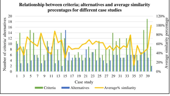
4.4 Calculations of case studies with original decision matrix included 56 4.4.1 The significance of the “similarity percentages” and the average “similarity percentages” ... 58
ix 4.4.2 Relationship between the number of criteria and the average
“similarity percentages” ... 59
4.4.3 Relationship between the number of alternatives and the average “similarity percentages” ... 60
4.4.4 The recommended number of criteria ... 61
4.4.5 The recommended number of alternatives ... 62
4.4.6 Summary on the case studies with original decision matrix included ………..63
4.5 Possible sources of error ... 63
4.5.1 Errors associated with long calculations ... 63
4.5.2 Errors associated with zero-values in the decision matrix ... 64
4.5.3 Errors associated with limitations of the MCDA techniques used ………..64
4.5.4 Errors associated with limited information supplied in the case studies ………..65
4.5.5 Summary on the possible sources of error ... 66
4.6 The MCDA techniques as assistance in decision making ... 66
4.7 Chapter summary ... 66
5 CONCLUSIONS AND RECOMMENDATIONS ... 68
5.1 Introduction ... 68
5.2 Findings of the research study ... 68
x 5.4 Recommendations for future work ... 71 6 REFERENCES ... 72
6.2 The following references do not appear in the main text but they are used as sources of data in Appendices 7-1 to 1-11 ... 82 7.2 Case studies and their corresponding criteria; alternatives; and average similarity percentages ... 87
xi
LIST OF FIGURES
Figure Page Figure 1-1 Different stakeholders in the mining industry ... 1 Figure 1-2: Qualitative and quantitative analysis in problem solving ... 5 Figure 1-3 Graphical presentation of the report structure ... 7 Figure 2-1 MCDA techniques used in the case study and their frequency of use 20 Figure 2-2 Usage frequency of different MCDA techniques in the combination of MCDA techniques ... 21 Figure 2-3 Different approaches of dealing with uncertainty in different published MCDA case studies ... 22 Figure 3-1 Flow process diagram for selection of case studies ... 42 Figure 4-1 The growth rate in USD for Chile; Australia; Peru and South Africa 53 Figure 4-2 Different MCDA techniques used in the identified case studies and their publication years ... 54 Figure 4-3 Relationship between criteria; alternatives and average similarity percentages for different case studies ... 57 Figure 4-4 Number of criteria plotted against average similarity percentages for the case studies ... 59 Figure 4-5 Number of alternatives plotted against average similarity percentages for the case studies ... 60
xii
LIST OF TABLES
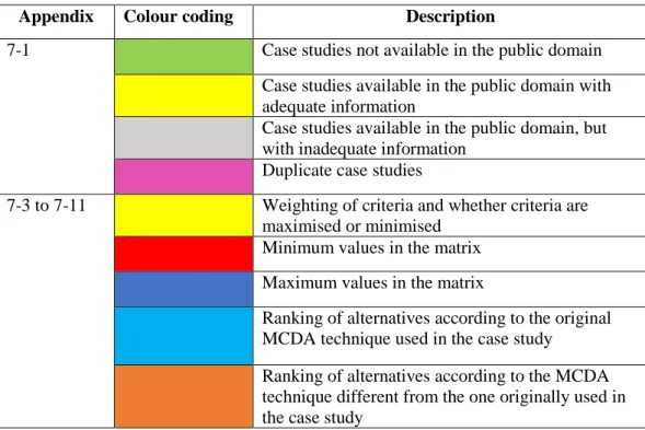
Table Page Table 2-1 The structure of a generic multi-criteria decision analysis problem... 9 Table 2-2 Summary of MCDM methods (adapted from Velasquez and Hester, 2013) ... 14 Table 2-3 Comparison of the five multi-criteria decision analysis methodology categories... 17 Table 3-1 Generic similarity percentages of alternatives ranked using three MCDA methods ... 45 Table 3-2 Generic colour coding used and their descriptions ... 46
xiii
LIST OF ACRONYMS
AHP: Analytic Hierarchy Process ANP: Analytic Network Process CBR: Case Based Reasoning CI: Consistency Index
CP: Compromise Programming CR: Consistency Ratio
DEA: Data Envelopment Analysis GFC: Global Financial Crisis
ELECTRE: Elimination and Choice Expressing Reality
MACBETH: Measuring Attractiveness by a Categorical Based Evaluation Technique
MADM: Multi-Attribute Decision Making MCDM: Mutli-Attribute Decision Making MODM: Multi Objective Decision Making MCDA: Multi-Criteria Decision Making MCQA: Multi-Criteria Q-Analysis
NAIADE: Novel Approach to Imprecise Assessment and Decision Environment
PROMETHEE: Preference Ranking Organisation Method for Enrichment Evaluation
RI: Random Index
xiv SMART: Simple Multi-Attribute Rating Technique
TOMASO: Technique for Ordinal Multi-Attribute Sorting and Ordering TOPSIS: Technique for Order Preference Similarity to Ideal Solution USD: United States Dollar
UTA: Utilities Additives method WP: Weighted Product
1
1
INTRODUCTION
1.1
Background
Natural resources are present in a country to serve the needs of different groups of people within the country, wherein the different groups are known as stakeholders. To address the varying needs of the stakeholders, these natural resources have to be managed optimally. In order to manage these resources, Multi-Criteria Decision Analysis (MCDA) techniques have been used. The techniques have been used to simultaneously integrate all the different needs and preferences of stakeholders (Herath and Prato, 2006).
Mining is no exception to the above, considering the fact that minerals are exploited for the benefit of different stakeholders. The stakeholders include the immediate community; employers; employees; shareholders; and government. Figure 1-1 shows the different stakeholders in the South African mining industry. Figure 1-1 also shows impacts of the stakeholders, their expectations and expected roles.
Figure 1-1 Different stakeholders in the mining industry
2 Resource management often involves decision making and one of the biggest challenges of decision making in mining is the one which Saaty (2007) called the “unknown future”. This ‘unknown future’ is characterised by uncertainty of what challenges the future will present. Businessdictionary.com defines uncertainty as: Decision making: Situation where the current state of knowledge is such that (1) the order or nature of things is unknown, (2) the consequences, extent, or magnitude of circumstances, conditions, or events is unpredictable and (3) credible probabilities to possible outcomes cannot be assigned. Although too much uncertainty is undesirable manageable uncertainty provides the freedom to make creative decisions. Information theory: Degree to which available choices or the outcomes of possible alternatives are free from constraints (WebFinance Inc., 2017).
According to Ernst & Young (2016), the top ten risks facing mining and metals companies in South Africa, in descending order of ranking are:
• The decision whether to buy or invest to acquire competitive advantage;
• Productivity improvement;
• Access to capital and challenging fundraising conditions;
• Resource nationalism through mandated beneficiation and increased taxes;
• Social license to operate;
• Volatility of the South African currency and commodity prices;
• Capital project allocation execution risk associated with cost and schedule overruns;
• Access to energy due to rising energy prices;
• Cyber security in a digital world; and
• Lagging innovation.
In order to address the challenge of uncertainty, scenario planning is used where mine planners consider multiple possible scenarios before a decision can be taken (Petit and Fraser, 2013; Saaty, 2007). Matos (2007) further defined scenario
3 planning as a way of modelling uncertainty, whereby the most likely future scenarios are expressed in qualitative ways.
In order to select the best scenario amongst other identified scenarios, multiple criteria and different alternatives are used together with the decision maker’s judgement for the overall decision making process. This is achieved by using MCDA methods, where different criteria and alternatives are assigned numerical values to derive an optimal outcome (Petit and Fraser, 2013).
1.2
Problem statement and motivation
The increasing amount of uncertainty and competitiveness of the global market has forced companies to increase their levels of efficiency, responsiveness and flexibility (Oliveira et al, 2013). To achieve these increased levels, the most decisive step was turning to MCDA methods to aid in strategic decision making, as human judgement is considered as “limited” when several criteria and alternatives need to be evaluated simultaneously.
The shift is evident as there are several research studies conducted on MCDA methods which were pioneered as early as the 1970s (Oliveira et al, 2013). These research studies have seen the development of various MCDA methods and differentiation of these methods. These methods have been used to address everyday problems faced in the mining industry and to yield acceptable solutions. For this research study, as many as 246 mine planning and related case studies were identified. From these case studies, between one and four MCDA techniques were used to solve the individual case studies. This gives rise to questions which the research report seeks to answer: “How appropriate is the MCDA method used with increasing number of criteria and alternatives? What is the most suitable number of criteria and alternatives to use when using MCDA techniques?”
4 Other applicable methods not used in a particular case study were utilised to validate the results yielded by the methods used. This research study also shows the applicability of these methods as the number of alternatives and criteria changes. The effectiveness of each method with increasing criteria and alternatives were then observed and accounted for.
1.3
Significance of the research study
Yavuz (2015b) defined Decision Making (DM) as a selection process for the best alternative in order to obtain a defined goal under conditions of uncertainty. DM is divided into structuring of problems and analysis of problems. In structuring of problems, a problem is defined and then the criteria and alternatives are identified and determined. In the analysis of problems, either qualitative or quantitative analysis is used to determine the appropriate decision to be taken (Yavuz, 2015b). In some instances, both qualitative and quantitative analysis may be used concurrently to solve a problem.
Both qualitative and quantitative analyses are essential in problem solving. According to Kazakidis et al (2004), qualitative analysis is mainly based on expert knowledge and experience and it is used if the analytical team has extensive experience to make informed judgements. Quantitative analysis is used where there is limited experience or a problem to be addressed is more complex (Kazakidis et al, 2004). In this analysis, facts or data collected together with a mathematical formula that includes the objectives; variables; and constraints of a problem are used. Figure 1-2 shows the relationship between problem structuring and problem analysis in problem solving.
5 Figure 1-2: Qualitative and quantitative analysis in problem solving
Source: Kazakidis et al (2004)
From Figure 1-2, quantitative analysis is analogous to literature work done by authors comparing the different MCDA methods and stating their advantages; disadvantages; and applications. This research study will be used to provide results for quantitative analysis. Once quantitative and qualitative analyses of the case studies have been conducted, an evaluation and a decision will be made. Evaluation and decision making includes observing the behaviour of different methods with each case study; and comparing the ranking of different alternatives as determined by different MCDA techniques.
The similarities observed when ranking alternatives will be utilised to determine the ideal number of criteria and alternatives to use in decision making with MCDA
6 techniques. This research study will recommend the ideal number of criteria and alternatives to use in decision making as means of reducing uncertainty. The recommended number of criteria and alternatives will in turn give the decision maker (mine planners and other practitioners) a level of confidence during the decision making process.
1.4
Objectives of the research study
The objectives of the research study are to:
• Establish the trend when different MCDA methods are used to solve the identified cases;
• Determine the appropriate method to use when the number of criteria and alternatives increases;
• Validate the results obtained with existing literature by various authors; and
• Determine the ideal number of criteria and alternatives to use when making decisions under uncertainty using MCDA techniques.
1.5
Structure of the research report
In order to achieve the objectives of the research study as stated in Section 1.4, the report is divided into five chapters. Chapter 1 has introduced background information on decision making in an uncertain mining environment and has provided the problem statement. Chapter 2 reviews the literature focusing on the MCDA methods considered in the study. The criteria used to select the MCDA methods are also discussed. Chapter 3 presents the selected case studies and the methodology used for their selection. Chapter 3 also introduces “similarity percentages” and how they are used for analysis of the case studies.
Results and analysis are presented in Chapter 4 where case studies are analysed in terms of the criteria; alternatives; and “similarity percentages”. Conclusions and
7 recommendations are made in Chapter 5. The graphical presentation of the outline of different chapters within the research report is indicated in Figure 1-3.
8
2
LITERATURE REVIEW
2.1
Introduction
This chapter presents the literature related to the different MCDA methods. It aims to indicate the significance of this study in relation to existing literature and it discusses in detail the methods selected for analysis. Chapter 2 also explains the selection process of the methods chosen. Frequency of use of the MCDA techniques as identified by different authors were used to select the methods.
2.2
Multi-criteria decision analysis
Decision making using multiple criteria and alternatives, for instance MCDA techniques, has shown to be reliable in an uncertain environment. MCDA techniques are a class of Multi-Criteria Decision Making (MCDM). MCDM is a process used to solve problems with more than one objective (Pohekar and Ramachandran, 2003). The solution determined depends on the preference of the decision maker. MCDM is divided into Multi Objective Decision Making (MODM) and Multi-Criteria Decision Analysis (MCDA) techniques. MODM techniques are used to address problems with an infinite number of alternatives (Musingwini, 2010).
MCDA techniques are used to solve problems with a finite number of alternatives that are selected from a set of established alternatives. These techniques are also known as Multi-Attribute Decision Making (MADM) techniques (Musingwini, 2010). This research study focuses on established cases with a defined number of alternatives hence MCDA techniques will be used for analysis. MCDA implementation in problem solving is in four steps and these steps are (Musingwini, 2010):
1. Identifying objectives and representing them as criteria; 2. Assigning numerical value or weights to the criteria;
9 3. Measuring the efficiencies of alternatives against different criteria to yield
outcomes; and
4. Making an appropriate decision from the outcome.
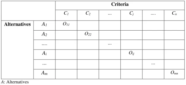
To yield an outcome an alternative Ai is selected from a set of alternatives A = {A1, A2, ……., Am}. Alternative Ai is measured against a decision criterion Cj from a set of criteria C = {C1, C2, ……, Cn}. An outcome, Oij is determined by measuring the efficiency of Ai against Cj. For m alternatives and n criteria, the alternatives and criteria are arranged in a (m x n) matrix to yield outcomes, as shown in Table 2-1. Table 2-1 The structure of a generic multi-criteria decision analysis problem
Criteria C1 C2 … Cj …. Cn Alternatives A1 O11 A2 O22 …. … Ai Oij … … Am Omn A: Alternatives C: Criteria
O: Outcome of measuring the efficiency of thealternative A in terms of criterion C
Source: Musingwini (2010)
2.3
Literature on MCDA methods
There are various MCDA methods that can be used to aid in decision-making. These methods are identified and categorised into different categories where classification may vary according to individual authors. Although the classification is unique for each author, there are common methods identified. The aim of this section is to review the categories and common methods, as presented by various authors. The
10 seven authors that were considered were Fülöp (2005); Figueira et al (2005); Sanandaji (2006); Peniwati (2007); Velasquez and Hester (2013); De Montis et al (2008); and Musingwini (2010). These authors were considered as they reviewed the different methods and associated categories.
2.3.1 Classification on a study by Fülöp in 2005
Fülöp (2005) defined multi-attribute decision problems as problems that have a finite number of criteria and alternatives. To solve such problems, Multi-Attribute Decision Making (MADM) methods are used. Fülöp (2005) classified MADM methods into Cost-Benefit Analysis (CBA); Elementary methods; Multi-Attribute Utility Theory (MAUT) methods; outranking methods; group decision making methods; and sensitivity analysis.
Elementary methods were further sub-divided using pros and cons analysis; minimum and maximum methods; conjunctive and disjunctive methods; and lexicographic methods (Fülöp, 2005). These methods were considered to be simple and not data-intensive. They also needed a single decision-maker. A single decision maker is required where decisions are less complex and the method used is simple, such as selection of the best alternative between two alternatives that yield the same outcome.
The MAUT methods were methods which had alternatives measured against different criteria. Numerical values assigned to different criteria were used to determine the importance of criteria in a decision (Fülöp, 2005). They were classified into Simple Multi-Attribute Rating Technique (SMART); generalised means; and the Analytic Hierarchy Process (AHP).
Fülöp (2005) defined outranking methods as those methods which compare the performance of two alternatives under a criterion. Outranking methods were divided into Preference Ranking Organisation Method for Enrichment Evaluation
11 (PROMETHEE); and Elimination and Choice Expressing Reality (ELECTRE) methods (Fülöp, 2005).
2.3.2 Classification by Figueira et al in 2005
Figueira et al (2005) classified outranking based multiple criteria decision making methods based on pairwise comparison of actions. These methods were divided into outranking methods; Multi-Attribute Utility and Value Theories (MAUT/ MAVT); and non-classical MCDA approaches. The outranking methods were further divided into ELECTRE methods; PROMETHEE methods; pairwise criterion comparison approach; and one outranking method for stochastic data.
MAUT/ MAVT were further divided into MAUT method; Utilities Additives (UTA) method; Analytic Network Process (ANP); AHP; and Measuring Attractiveness by a Categorical Based Evaluation Technique (MACBETH) (Figueira et al, 2005). Non-classical MCDA approaches were introduced to account for any uncertainties associated with a changing environment. Under non-classical MCDA approaches the Fuzzy set approach; and Technique for Ordinal Multi-Attribute Sorting and Ordering (TOMASO) tool-based software were placed (Figueira et al, 2005).
2.3.3 Classification by Sanandaji in 2006
Sanandaji (2006) referred to decision making methods as models and classified them into Multi-Criteria Decision Making (MCDM); Multi-Attribute Decision Making (MADM); rational decision making; irrational decision making; and non-rational decision making models. The MCDM was further divided into ELECTRE-2; PROMETHEE-ELECTRE-2; AHP; Compromise Programming (CP); and Multi-Criteria Q-Analysis (MCQA). MADM was subdivided into Simple Additive Weighing (SAW) method; Weighted Product (WP) method; and Technique for Order Preference Similarity to Ideal Solution (TOPSIS) method. For each of the decision making classes, the advantages and disadvantages were discussed by Sanandaji (2006).
12 2.3.4 Classification by Peniwati in 2007
Peniwati (2007) identified fifteen MCDA methods. These methods were divided into three classes namely structuring methods; ordering and ranking methods; and structuring and measuring methods. Structural problems are explained as those problems where key words are used to establish a relationship between analogies and the problem. Analogy association; boundary examination; brainstorming/brain writing; morphological connection; and why-what’s stopping methods were put under this class.
Structuring and measuring methods consisted of Bayesian analysis; MAUT; and AHP (Peniwati, 2007). In this class of methods, different alternatives were established and summed up to rank criteria. Ordering and ranking methods included voting method; nominal group technique; Delphi technique; disjointed incrementalism; matrix evaluation; goal programming; conjoint analysis; and outranking methods. These methods were considered as single criterion analysis methods (Peniwati, 2007).
2.3.5 Classification by other authors
Velasquez and Hester (2013) conducted a study with the aim of identifying MCDA methods and their applications. They used databases like Springer; ScienceDirect; IEEExplore; journal articles; and conference proceedings to identify publications on MCDA. The identified publications were narrowed to publications of the most commonly used methods. The identified case studies were grouped according to the frequency of usage of the MCDA techniques. MAUT; AHP; Fuzzy set theory; Case Based Reasoning (CBR); and Data Envelopment Analysis (DEA) were identified. Simple Multi Attribute Rating Technique (SMART); goal programming; ELECTRE; PROMETHEE; SAW; and TOPSIS methods were also identified. MAUT was the most frequently used method amongst all of the identified methods. MAUT was also mostly used with other methods when two or more methods were
13 utilised. Two or more methods were used so that an alternative method could make up for the shortcomings of a particular method. The advantages; disadvantages and applications of the identified methods are tabulated in Table 2-2.
14 Table 2-2 Summary of MCDM methods (adapted from Velasquez and Hester, 2013)
Method Advantages Disadvantages Application
Multi-Attribute Utility Theory (MAUT)
Takes uncertainty into account; can incorporate preferences
Needs a lot of input; preferences need to be precise
Economics; business and finance; actuarial; water management, energy management
Analytical Hierarchy Process (AHP)
Easy to use; scalable; hierarchy structure can easily adjust to fit many sized problems; not data intensive
Problems due to interdependence between criteria and alternatives; can lead to inconsistencies between judgement and ranking criteria; rank reversal
Performance-type problems; resource management, corporate policy and strategy; public policy; political strategy; and planning
Case Based Reasoning (CBR) Not data intensive; requires little maintenance; can improve over time; can adapt to changes over the environment
Sensitive to inconsistent data; requires many cases
Businesses and finance; vehicle insurance; healthcare; and engineering design
Data Envelopment Analysis (DEA)
Capable of handling multiple inputs and outputs; efficiency can be analysed and quantified.
Does not deal with imprecise data; assumes that all input and output are exactly known.
Economics; healthcare; utilities; road safety; agriculture; business and finance
Fuzzy set theory Allows for imprecise input; takes into account insufficient information
Difficult to develop; can require numerous simulations before use
Engineering; economics; environmental; social; healthcare and management
Simple Multi Attribute Ranking Technique (SMART)
Simple; allows for any type of weight assessment technique; less effort by decision makers
Procedure may not be convenient to solve problems in a real-life situation
Environmental; construction; transportation and logistics; military; manufacturing and assembly problems
Goal Programming (GP) Capable of handling large-scale problems; can produce infinite alternatives
Cannot generate weight coefficients hence it typically needs to be used in combination with other MCDM methods to yield weight coefficients
Production planning; scheduling; healthcare; portfolio selection; distribution systems; energy planning; water reservoir management; scheduling and wildlife management
Elimination and Choice Expressing Reality (ELECTRE)
Takes uncertainty and vagueness into account Its process and outcome can be difficult to explain in layman’s terms; outranking causes the strengths and weaknesses of the alternatives to not be directly identified
Energy; economics and business; environmental; water management; and transportation problems
Preference Ranking Organization Method for Enrichment Evaluation (PROMETHEE)
Easy to use; does not require assumption that criteria are proportional
Does not provide a clear method by which to assign weights
Environmental; hydrology; water management; business and finance; chemistry; logistics and transportation; manufacturing and assembly; energy; agriculture
Simple Additive Weighting Ability to compensate among criteria; intuitive to decision makers; calculation is simple and does not require complex computer programs
Estimates revealed do not always reflect the real situation; result obtained may not be logical
Water management; business and finance
Technique for Order Preference Similarity to Ideal Solution (TOPSIS)
Has a simple process; easy to use and program; the number of steps remains the same regardless of the number of attributes
Its use of Euclidean distance does not consider the correlation of attributes; difficult to weight and keep consistency of judgement
Supply chain management and logistics; engineering; manufacturing systems; business and finance; environmental; human resources; and water resources management
15 De Montis et al (2008) established that environmental problems are characterised by high risks; high stakes; urgency; and dispute. To solve environmental problems, De Montis et al (2008) identified and analysed the most commonly used MCDA methods. There were seven methods identified from this analysis and they were assessed in terms of their use and application. The classification of the methods was made into single criterion methods; outranking methods; and programming methods.
De Montis et al (2008) in their classification, defined single criterion approach methods as methods where a single attribute is generated from different criteria. The single attribute is used to compare different alternatives. Single criterion approach methods were classified into CBA; MAUT; AHP; and Evaluation matrix (Evamix).
ELECTRE III; Regime; and Novel Approach to Imprecise Assessment and Decision Environments (NAIADE) were classified under outranking methods. These were methods in which the decision maker may change preference based on the available information (De Montis et al, 2008). Programming methods were methods where mathematically formulated alternatives were generated as part of the solution. Programming methods were divided into goal programming and multiple objective programming.
Musingwini (2010) identified five most commonly used MCDA techniques based on the frequency of the techniques used not only in other sectors, but also in the mining industry. The frequency of usage of different MCDA techniques was narrowed down to the mining industry. The identified techniques were MAUT; AHP; ELECTRE; PROMETHEE; and TOPSIS. These techniques were compared under criteria of foundation; theoretical basis; measurement criteria; and determination of weights of criteria.
Table 2-3 shows a summary of the different methodologies compared under the different criteria. Musingwini (2010) identified AHP as the most frequently used
16 MCDA technique for solving mining-related problems. MCDA methods are progressively used for solving problems and their successful use has given decision makers confidence when dealing with uncertainty in the mining industry. From Tables 2-2 and 2-3, it is noticeable that different MCDA methods are used to address various problems and they all have unique properties.
17 Table 2-3 Comparison of the five multi-criteria decision analysis methodology categories
Multiple Attribute Utility Theory (MAUT)
Analytical Hierarchy Process (AHP)
Elimination and Choice Expressing Reality (ELECTRE)
Preference Ranking Organization Method for Enrichment Evaluation (PROMETHEE)
Technique for Order Preference Similarity to Ideal Solution (TOPSIS)
Foundation Classical MCDA
approach
Classical MCDA but hierarchical approach
Outranking procedure Outranking procedure Classical MCDA approach Theoretical basis Utility function additive model Pair-wise comparison (weighted eigenvector evaluation) Pair-wise comparison (concordance analysis) Pair-wise comparison (preference function) Dimensionless Euclidean space evaluation model Measurement of criteria Numerical (non-numerical data must be converted to numerical scale)
Numerical (non-numerical data must be converted to numerical scale)
Numerical (non-numerical data must be converted to numerical scale)
Numerical (non-numerical data must be converted to numerical scale)
Numerical (non-numerical data must be converted to a dimensionless numerical scale) Determination of weights of criteria Trade-off based weights (generate weights using swing, direct-ratio, or Eigenvector methods)
Trade-off (generate weights using Saaty’s Eigenvector and geometric mean)
Non-trade-off (does not provide procedure to obtain weights)
Non-trade-off (does not provide procedure to obtain weights)
Trade-off based weights
Result Relative preference
order
Relative preference order
A set of non-dominated alternatives
Partial and complete ranking order
Relative preference order
18 2.4 Approach to selecting MCDA methods
The choice of MCDA methods to be used in this research study was based on two factors:
• The extent of use of the method, as shown by the seven authors discussed previously in Section 2.3; and
• The extent of use of the method to solve the identified mine planning; and related case studies.
All the seven authors, as indicated in Section 2.3, through varying methods of classification, identified AHP; MAUT; PROMETHEE; and ELECTRE as the most commonly used methods. Figueira et al (2005) and Peniwati (2007) had outranking methods as a common class of methods. ELECTRE and PROMETHEE methods were found in this class. In addition, Sanandaji (2006) and Musingwini (2010) identified TOPSIS as one of the frequently used methods. Figueira et al (2005) introduced the fuzzy method as a way of accounting for uncertainty in problems that were addressed.
2.4.1 The extent of use for each technique in the identified case studies
Various journal and symposia papers were reviewed for choice of case studies. The journal and symposia papers presented different case studies where decisions were made with different MCDA techniques. The scope of case studies was narrowed down to case studies on mine planning and those related to mine planning. Case studies were narrowed down to mine planning in order to show the:
• Extent of use of MCDA techniques in mine planning, in terms of decision making;
• Progression of MCDA techniques over the years; and
• The different levels of planning where MCDA techniques have been applied.
19 Not all of the papers on mine planning and related case studies were available in the public domain. The papers that were unavailable were from the China Knowledge Resource Integrated database website (www.cnki.net) and registration request to the database led to a denied access. The available papers were sourced from different journals and portals like Researchgate.net. The identified journals and symposia papers were published in different areas of mine planning. The following areas were identified within the case studies:
• Strategic mine planning;
• Economic aspects in mine planning;
• Mining method selection;
• Location of facilities (tailings dams; processing plants; crushers);
• Mining equipment selection (road headers, trucks);
• Selection of remedial sites for post mining activities; and
• Mining layout selection.
A total of 246 papers were identified and their years of publication was used to illustrate the use of MCDA techniques over the years. The years of publication range from 1984 to 2016, as shown in Appendix 7-1. Different MCDA techniques were used to rank alternatives in each case study. Figure 2-1 shows the frequency of use in raking different alternatives of case studies in the identified papers.
20 Figure 2-1 MCDA techniques used in the case study and their frequency of use
Figure 2-1 shows that the most frequently used MCDA techniques are AHP; ELECTRE; Fuzzy logic; TOPSIS; VIKOR and Yager’s method. The high frequency of usage for the techniques is attributed to the simplicity and ease of use of these techniques. The combination of the techniques was analysed to demonstrate which MCDA techniques are most frequently included in the combination.
A combination of techniques is used where one technique is used to assign weights to criteria and the other technique is used to rank alternatives. For instance, Stojanovic; Bogdanovic; and Urosevic (2015) (cited in Musingwini, 2016) selected the optimal technology for surface mining using AHP and ELECTRE. The weights of different criteria were determined using AHP while the alternatives were ranked using ELECTRE. Figure 2-2 depicts the frequency of different methods combined in the 55% combination of methods, as shown in Figure 2-1.
55% 28%
5% 2%
2% 1% 1% 1% 5%
MCDM methods used for analysis of the identified case studies
Combination of methods AHP Fuzzy set theory PROMETHEE TOPSIS Yager's method
21 Figure 2-2 Usage frequency of different MCDA techniques in the
combination of MCDA techniques
Figures 2-1 and 2-2 illustrate that the most frequently used MCDA techniques are AHP; Fuzzy logic; TOPSIS; PROMETHEE; VIKOR; ELECTRE; SAW; and Yager’s method. These techniques had a high frequency of use due to their simplicity and ease of use. These MCDA techniques were chosen for analysing the case studies because they do not require complex computation methods like software and reference can be made to the existing literature, in terms of their usage. AHP is most commonly used method for it accounts for consistency of matrices hence eliminating inconsistencies (Musingwini, 2016). AHP can be used with easily accessible software like Microsoft Excel and it ranks alternatives consistently.
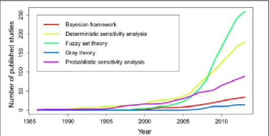
Broekhuizen et al (2015) selected case studies solved using MCDA techniques with publication years ranging from 1986 to 2013. The selected case studies were classified according to approaches used to address uncertainty. Five approaches were identified, namely; Bayesian framework; deterministic sensitivity analysis; Fuzzy set theory; Gray theory; and probabilistic sensitivity analysis. Fuzzy set
0 10 20 30 40 50 60 70 80 Fre q u en cy o f u se MCDA technique
Usage frequency of different MCDA techniques in the combination of techniques
22 theory was the most frequently identified approach, accounting for 45% of the case studies (Broekhuizen et al, 2015). Figure 2-3 illustrates the results from the study by Broekhuizen et al (2015).
Figure 2-3 Different approaches of dealing with uncertainty in different published MCDA case studies
Source: Broekhuizen et al (2015)
Figure 2-3 illustrates that Fuzzy logic is most frequently used to address uncertainty in MCDA techniques, not as an independent MCDA technique. The most commonly used MCDA techniques (Section 2.3.5) included MAUT, so MAUT was substituted for fuzzy set theory in the selected techniques for analysis.
2.5
MCDAtechniques selected to analyse the case studies
A total of eight MCDA techniques were selected for analysis of the case studies. SAW; PROMETHEE; MAUT; TOPSIS; VIKOR; AHP; and Yager’s method are the eight selected techniques. The principle behind these techniques is discussed at length in Sections 2.5.1 to 2.5.8.
23 2.5.1 Simple Additive Weighting (SAW)
The Simple Additive Weighting (SAW) method is one of the most widely used technique because of its simplicity (Memariani et al, 2009). It is an important technique because it forms the basis of methods such as AHP and PROMETHEE in terms of calculating scores used to rank alternatives. The SAW method involves calculating normalized values for each alternative in a decision matrix. Equation 2-1 shows how normalized values for a normalized decision matrix, R are calculated (Memariani et al, 2009):
𝑟𝑖𝑗 = 𝑥𝑖𝑗
𝑚𝑎𝑥(𝑥𝑗) 2-1
Where xij is the value assigned for alternative Ai in criterion Cj in the original decision matrix X; max xj is the maximum xij value in criterion Cj; and rij is the normalized value for alternative Ai in criterion Cj of matrix X. Equation 2-1 holds for criteria to be maximized while in criteria to be minimized Equation 2-2 holds (Memariani et al, 2009):
𝑟𝑖𝑗 = 𝑚𝑖𝑛(𝑥𝑖)
𝑥𝑖𝑗
2-2
Where xij is the value assigned for alternative Ai in criterion Cj in the original decision matrix X; min xjis the minimum xij value in criterion Cj and rij is the normalized value for alternative Ai in criterion Cj of the original decision matrix X. For an alternative Ai, each normalized value rij is multiplied by weightings assigned to different criteria (Wj) and the sum of the product (Wj* rij) yields a weighted score for each alternative, Vi. Equation 2-3 illustrates how Vi is calculated (Memariani et al, 2009):
24 The weighted score, Vi, is used to rank different alternatives. The higher the value of Vi, the higher the ranking of the alternative. The advantage of the SAW method is that it is easy to use due to its simplicity (Velasquez and Hester, 2013). The disadvantage of the SAW is that the calculations seldom yield solutions that do not reflect the practical situations (Velasquez and Hester, 2013).
2.5.2 Preference Ranking Organisation Method for Enrichment Evaluation (PROMETHEE)
Preference Ranking Organisation Method for Enrichment Evaluation (PROMETHEE) is an MCDA method that was developed by Brans in 1982. It was further modified by Brans and Mareschal in 1994 (Kasperczyk and Knickel, n.d.). Elevli and Demicri (2004) described PROMETHEE as a method that is:
• Easy to understand, making it easy for the user or decision maker to understand the mathematics behind the method, yielding results that are transparent and can be easily scrutinised by parties other than the decision maker; and
• Easy to use since two parameters of the function are associated with the criterion to yield a single-valued outranking related to this criterion. When two alternatives cannot be compared in terms of preference or indifference then the two alternatives are said to be incomparable.
PROMETHEE is considered as an outranking method (Kasperczyk and Knickel, n.d.). A matrix V, consisting of vij elements is constructed, where a performance value of alternative Ai under criterion Cj, vij is shown, for i = 1, ……, m and j = 1, ….. ,n. A matrix K is constructed from matrix V, where kij shows the utility of alternative Ai, based on criteria Cj and its relationship with vij is shown in Equation 2-4 (Elevli and Demicri, 2004):
25 The utility kij has values that lie between 0 and 1. A matrix G of quantitative weights of different criteria is also constructed where it represents weights (g) of different criteria, from 1 to j. When the three matrices V, K and G have been constructed, each alternative is ranked using Equation 2-5 (Elevli and Demicri, 2004):
𝑁 = 𝐾 ∗ 𝐺 2-5 Where N is a vector that shows the overall benefit of each alternative. After determining N, PROMETHEE is utilised in two stages. The first stage, PROMETHEE I is used for partial pre-order ranking of alternatives. PROMETHEE II is the last stage utilised for complete ranking of alternatives (Elevli and Demicri, 2004).
During the comparison of alternatives, a preference function, P(xi,xk) is used to represent the intensity of the preference of alternative xi over alternative xk,, where
k ϵ (1, 2, …..n). Different types of preferences are represented thus (Elevli and Demicri, 2004):
• P(xi,xk) = 0 shows indifference or no preference of alternative xi, over alternative xk
• P(xi,xk) ~ 0 shows weak preference of xi over xk
• P(xi,xk) ~ 1 shows strong preference of xi over xk
• P(xi,xk) = 1 shows strict preference of xi over xk
The generalized criterion function of two alternatives i and k, H(dik) is used and it is represented in Equation 2-6:
𝐻(𝑑𝑖𝑘) = {0𝑖𝑓𝑑𝑖𝑘 = 0
1𝑖𝑓𝑑𝑖𝑘 ≠ 0 2-6 Where dik = v(xi) – v(xk) is the deviation between two criteria v(xi) and v(xk) associated with alternatives Ai and Ak, respectively (Deshmukh, 2013). From
26 preferences, a preference index is established to define the intensity of the decision maker’s preference for xi over xk , Π(xi,xk). The preference index is shown by Equation 2-7 as (Elevli and Demicri, 2004):
𝛱(𝑥𝑖𝑥𝑘) = ∑ 𝑤𝑗∗
𝑘
𝑗=1 𝑃(𝑥𝑖,𝑥𝑘)
∑𝑘𝑗=1𝑤𝑗
2-7
Where wj is the weighted average for criterion Cj. Similar to Equation 2-4, the
preference index lies between 0 and 1, therefore the following holds (Elevli and Demicri, 2004):
• 𝐻(𝑑𝑖𝑘) ~ 0 shows weak preference of alternative xi over xk;
• 𝐻(𝑑𝑖𝑘) ~ 1 shows strong preference of alternative xi over xk for all criteria.
The preference index is used to determine the positive preference flow to measure an outranking character and negative preference flow to measure an outranked character for an alternative, as indicated by Equations 2-8 and 2-9 (Elevli and Demicri, 2004):
Ф+(𝑥𝑖) = ∑𝑚𝑘=1𝛱(𝑥𝑖𝑥𝑘) 2-8
and
Ф−(𝑥
𝑖) = ∑𝑚𝑘=1𝛱(𝑥𝑘𝑥𝑖) 2-9
The difference between the positive preference flow (Equation 2-8) and negative preference flow (Equation 2-9) is called net flow (Elevli and Demicri, 2004). Equation 2-10 represents the net flow or the net preference of an alternative Ai, which is calculated as shown:
27 Net flow is characteristic of PROMETHEE II, which is used for complete ranking of alternatives (Deshmukh, 2013). PROMETHEE II also ranks all the alternatives, from the best to the worst. If, for alternatives i and k, Ф(xi) is greater than Ф(xk) then alternative i is preferred. If Ф(xi) is equal to Ф(xk) then the alternatives are said to be indifferent from each other (Elevli & Demicri, 2004). The preference is important for it is used to evaluate the alternatives.
2.5.3 Multi-Attribute Utility Theory (MAUT)
Liu (2015) described the Multi-Attribute Utility Theory (MAUT) as one of the most widely used methodologies in multiple attribute decision making processes. MAUT is used to compare multiple attributes, by assigning numerical values (utilities) to objectives and giving them unit scales. Unit scales are assigned to allow for comparison under uniform conditions. Attributes (or criteria) being compared can either complement each other or substitute each other. MAUT provides the decision maker with qualitative and quantitative analysis to justify the chosen alternatives, given the existing criteria (Collins et al, 2006).
In MAUT, two extremes or conditions ranging from 0 to 1 are established, with 0 being the worst and 1 being the best. From there, utility functions of criteria lying between two extremes are established with respect to the best and worst values (or extremes) and weight assessments are made (Liu, 2015). Utilities can be determined through addition (additive utility) or multiplication (multiplicative utility). The aim of this method is to maximize the combined utility values in order to make the best decision.
The utility function, 𝑈(𝑥) for an attribute under a specific alternative is calculated using Equation 2-11:
𝑈(𝑥) = 𝑥−𝑥𝑖−
28 Where xi- is the value of attribute xi under the worst alternative; xi+ is the value of attribute xi under the best alternative; and x is a value of attribute xi under a specific alternative (Liu, 2015). Relative weights of attributes (ki) are calculated by comparison of attributes and generating ratios such that 0 ≤ ki ≤ 1 and ∑ ki = 1 (Liu, 2015).
The relative weights are then multiplied by the individual utility functions to determine their utility, hence their ranking (Liu, 2015). The utility (U) is calculated as shown by Equation 2-12:
𝑈 = ∑𝑚𝑖=1𝑘𝑖 ∗ 𝑈𝑖(𝑥) 2-12 Where ki is the relative weight of the ith attribute and Ui(x) is the utility function of
the ith attribute where 0 ≤ Ui (x) ≤1. The alternative with the highest utility value is the one taken for consideration. The type of utility in Equation 2-12 is called the additive utility and the attributes are dependent on each other (Collins et al, 2006). With multiplicative utility, on the other hand, the utility is determined using Equation 2-13:
𝑈 =
∏ [𝐾∗𝑘𝑖∗𝑈𝑖(𝑥)+1]𝑚 𝑖=1
𝐾 2-13
Where ki is the relative weight of attribute Ai and 0≤ ki ≤ 1; Ui(x) is the utility function of the ith attribute and K is a scaling constant that is determined as depicted in Equation 2-14:
1 + 𝐾 = ∏𝑚 (1 + (𝐾 ∗ 𝑘𝑖))
𝑖=1 2-14
K must be iteratively determined (Collins et al, 2006). In this utility, all attributes are independent of each other and -1 < K < 0 indicates utility independence (Collins et al, 2006). MAUT has an advantage of aiding the decision maker to develop practical preference criteria. MAUT also aids in determining which assumptions
29 are practical and in analysing the calculated utility functions (Velasquez and Hester, 2013).
2.5.4 Elimination and Choice Expressing Reality (ELECTRE)
The Elimination and Choice Expressing Reality or Elimination Et Choir Traduisant La Realite method is also known as ELECTRE method. It dates back as early as 1966, but only became widely known in 1968 (Buchanan and Sheppard, 1998). The ELECTRE is used when there are at least three criteria, in some instances from five to thirteen criteria to be compared. There are four sub-divisions of the method, namely ELECTRE I; II; III; and IV). ELECTRE usage consists of two main concepts which are threshold establishment and outranking a set of alternatives under defined criteria (Buchanan and Sheppard, 1998).
Firstly, for two alternatives a and b belonging to a set of alternatives A and defined criteria gj (where j =1, 2,….r) a preference is introduced. In a preference alternative a (or b) is either preferred to; indifferent to; or cannot be compared to b (or a). A preference is described thus (Buchanan and Sheppard, 1998):
• aPb : a is preferred to b, also presented by g(a) > g(b)
• aIb : a is indifferent to b, also presented by g(a) = g(b)
• aJb : a cannot be compared to b Secondly, the indifference threshold, q is derived and its purpose is to measure weak preference. It is characteristic of the decision maker since it incorporates how the decision maker feels about the comparison (Buchanan and Sheppard, 1998). The indifference threshold is incorporated into the traditional preference modelling, as shown in Equation 2-15:
• aPb – a is preferred to b, where g(a) > g(b) + q
30
• aJb – a is indifferent to b 2-15
Thirdly, a range or buffer between P (preference) and I (indifference) is created. This range or zone between the two extremes is known as the intermediary zone or the zone of weak preference (Buchanan and Sheppard, 1998). It is introduced to the preference model as a preference threshold, p. A “double threshold” model, is yielded where Q measures weak preference and P measures strong preference (Buchanan and Sheppard, 1998). Equation 2-16 represents the relationship between P and Q as:
• aPb – a is strongly preferred to b, where g(a) – g(b) > p
• aQb – a is weakly preferred to b, where q < g(a) – g(b) ≤ p
• aIb – a is indifferent to b and b to a; where |g(a) – g(b)| ≤ q 2-16 Once thresholds have been used to describe different models, the ELECTRE
method then builds an outranking relation, S. For instance, aSb means that at least a is as good as b, or a is not worse than b. For each of the criterion under study (j), aSjb means that a is good as b with respect to criterion j (Buchanan and Sheppard, 1998).
After S, two definitions, concordance and discordance, also known as harmony and disharmony respectively are introduced. A criterion j is in concordance with assertion aSb if “a is as good as b” or gj(a) ≥ gj(b) - qj even if gj(a) is less than gj(b) with a value of qj. A criterion j is in discordance with assertion aSb if b is strongly preferred to a, or gj(b) ≥ gj(a) + pj.
Concordance and discordance definitions seek to address whether, for a certain criterion j, and alternatives a and b there is a harmony or disharmony with the statement of whether a is as good as b (Buchanan and Sheppard, 1998). To quantify concordance and discordance of alternatives a and b and to measure the strength of assertion aSb, Concordance (C) indices are introduced, see Equation 2-17:
31 𝐶(𝑎, 𝑏) = 1
𝑘 𝑘𝑗𝑐𝑗(𝑎, 𝑏); 𝑤ℎ𝑒𝑟𝑒𝑘 = 𝑗=1𝑘𝑗 𝑟
𝑗=1𝑟 2-17
Where C(a,b) is the concordance index of alternatives (a, b) ∈ A; kj is the importance coefficient of criterion j and A is the set of all alternatives. Lastly, a discordance matrix is derived. In the same manner, a discordance matrix is derived from the discordance index. The discordance and concordance matrices are combined to form a credibility matrix, which is used to provide the assertion between alternatives a and b (Buchanan and Sheppard, 1998). The final ranking of alternatives is done with the credibility matrix and graph theory concepts.
ELECTRE methods account for uncertainties through creating thresholds and intermediary zones between two extreme preferences (Velasquez and Hester, 2013). Conversely, the intermediary zones are created to cover the strengths and weaknesses of the alternatives. ELECTRE methods may appear to be challenging to comprehend and not user friendly (Velasquez and Hester, 2013).
2.5.5 Technique for Order Preference by Similarity to Ideal Solutions (TOPSIS)
TOPSIS is a MCDA method that was first proposed by Hwang and Yoon in 1981 (Kabir and Hasin, 2012). TOPSIS is used to solve multiple attribute decision making problems. The assumption of TOPSIS is that each evaluation indicator has a feature that is either decreasing or increasing monotonically (Chen et al, 2015). TOPSIS is easy to implement and useful when the decision maker wants a simple weighting approach (Kabir and Hasin, 2012).
TOPSIS establishes a positive ideal solution composed of optimal values and a negative ideal solution consisting of the worst values for all indicators. The indicators established are compared to the two ideal solutions through the calculation of Euclean distances (Kabir and Hasin, 2012). The best solution has the shortest distance to the positive ideal solution and the longest distance to the
32 negative ideal solution (Chen et al, 2015). Kabir and Hasin (2012) defined the positive ideal solution as a solution that maximises the benefit criteria, while minimising the cost criteria. The contrary is true for the negative ideal solution. Firstly, for attributes (Cj, j = 1, 2,….., n) and alternatives (Ai, i = 1, 2,……, m), a normalised decision matrix is constructed, which allows for the comparison of attributes or criteria through giving them a comparable scale (Kabir and Hasin, 2012). Normalisation is calculated using Equation 2-18:
𝑟𝑖𝑗 = 𝑥𝑖𝑗
√∑𝑚𝑖=1𝑥𝑖𝑗2
2-18
Where rijis the normalised value of the performance attribute; and xij is an element of the matrix X indicating the performance of the ith alternative Ai with respect to the jth attribute Cj (Kabir and Hasin, 2012).
Secondly, a weighted normalised decision matrix is constructed for the criteria and a set of weights for the criteria Cj is assumed. Weighting is done to show the importance of a criterion relative to other criteria (Kabir and Hasin, 2012). Each column of the normalised matrix is multiplied with the corresponding weight wj to get a matrix of order m x n. Equation 2-19 shows how a weighted normalised value (or outcome), vij is calculated (Kabir and Hasin, 2012):
ʋ𝑖𝑗 = 𝑤𝑗𝑟𝑖𝑗, 𝑓𝑜𝑟𝑖 = 1, 2, … . . , 𝑚𝑎𝑛𝑑𝑗 = 1, 2, … … . , 𝑛 2-19 Where 𝑤𝑗is the relative importance of each attribute to the others; and 𝑟𝑖𝑗is the normalised value of the performance of attribute Ai with respect to criterion Cj. Thirdly, a negative ideal solution (A-) and a positive ideal solution (A+) are
developed. The ideal solutions are defined in terms of the weighted normalised values. To calculate a positive ideal solution (A+) and a negative ideal solution (A-) . Equations 2-20 and 2-21 are used respectively (Kabir and Hasin, 2012):
33
𝐴+= {ʋ1, . . . , ʋ𝑛}𝑤ℎ𝑒𝑟𝑒ʋ𝑗 = {𝑚𝑎𝑥(ʋ𝑖𝑗) 𝑖𝑓𝑗 ∈ 𝐽; 𝑚𝑖𝑛(ʋ𝑖𝑗) 𝑖𝑓𝑗 ∈ ǰ} 2-20 𝐴−= {ʋ1−, . . . , ʋ𝑛−}𝑤ℎ𝑒𝑟𝑒ύ𝑗 = {𝑚𝑖𝑛(ʋ𝑖𝑗) 𝑖𝑓𝑗 ∈ 𝐽; 𝑚𝑎𝑥(ʋ𝑖𝑗) 𝑖𝑓𝑗 ∈ ǰ} 2-21
Where J and ǰ are sets of benefit attributes and cost attributes, respectively. In an ideal situation, J is supposed to be larger than ǰ. Separation measures of each alternative (from the positive and negative ideal alternatives) Si+ and Si- are calculated using Equations 2-22 and 2-23:
𝑆𝑖+ = √∑𝑛𝑗=1(𝑣𝑖𝑗− 𝑣𝑗+)2 2-22
𝑆𝑖− = √∑𝑛 (𝑣𝑖𝑗 − 𝑣𝑗−)2
𝑗=1 2-23
For i = 1, 2, ….., m and the weight of each pair of alternatives Aii relative to criterion
Cj, given by vij.Equation 2-24 shows how the relative closeness or similarity of alternatives to the ideal solution 𝐶𝑖+ is calculated:
𝐶𝑖+ = 𝑆𝑖−
(𝑆𝑖++𝑆𝑖−), 0 < 𝐶𝑖
+ < 1 2-24
Thirdly, the alternatives are ranked by comparing 𝐶𝑖+ values. The alternative with the highest relative closeness to the ideal solution is taken as the best alternative (Kabir and Hasin, 2012). TOPSIS is user friendly, making it a commonly used method. The number of steps in problem solving is not affected by the varying number of criteria (Velasquez and Hester, 2013). The Euclean distance does not consider linked criteria. Consistent weighing of attributes is challenged when the number of criteria increases (Velasquez and Hester, 2013).
2.5.6 Vise Kriterijumska Optimizacija I Kompromisno Resenje (VIKOR) Vise Kriterijumska Optimizacija I Kompromisno Resenje (VIKOR) is a technique that was initially introduced by Serafim Opricovic in 1998 (Bulgurcu, 2016).
34 Opricovic and Tzeng further developed the VIKOR method and in 2004 it was fully recognised (Bulgurcu, 2016). VIKOR is an MCDA technique that aids in making a decision by comparing solutions to the ideal solution. The best solution is considered as the compromise solution and a solution closest to the compromise solution is considered to be the preferred solution (Bulgurcu, 2016).
Firstly, when using VIKOR, a decision matrix X is developed. The decision matrix is then normalised to yield a normalised matrix R and normalisation is conducted as shown in Equation 2-25 (Hayati et al, 2015):
𝑟𝑖𝑗 = 𝑥𝑖𝑗
√∑ 𝑥𝑖𝑗2
2-25
Where xij is the value assigned to alternative Ai in criterion Cj of matrix X; and rij is the normalised value for alternative Ai in criterion Cj in matrix R. Secondly, the normalised decision matrix R is multiplied with the corresponding weighting of criterion Cj (Wj) to obtain a weighted normalised matrix F, as shown in Equation 2-26 (Hayati et al, 2015):
𝑓𝑖𝑗 = 𝑥𝑖𝑗∗ 𝑊𝑖𝑗 2-26 Where fij is the weighted normalised value for matrix F. Thirdly, the ideal positive fj*and ideal negative fj- solutions are determined. For a criterion to be maximised fj* is the maximum value of fij and fj- is the minimum value of fij for criterion Cj. For a criterion to be minimised, fj* is the minimum value of fij and fj- is the maximum value of fij for criterion Cj (Hayati et al, 2015).
The calculated ideal solutions are used to determine the satisfaction (Si) and rejection (Ri) indices (Hayati et al, 2015). Si shows the distance of an alternative to the ideal positive value, while Ri shows the maximum distance from the ideal positive value. Equation 2-27 demonstrates how Ri and Si are calculated (Hayati et al, 2015):
35 𝑆𝑖 = ∑ 𝑊𝑗∗ 𝑓𝑗∗−𝑓𝑖𝑗 𝑓𝑗∗−𝑓𝑗−𝑎𝑛𝑑𝑅𝑖 = 𝑚𝑎𝑥 [𝑊𝑗∗ 𝑓𝑗∗−𝑓𝑖𝑗 𝑓𝑗∗−𝑓𝑗−] 2-27
Lastly, for each alternative Ai, the VIKOR index (Qi) has to be calculated. Q considers the satisfaction and rejection indices, together with a ranking constant. Q is calculated according to Equation 2-28 (Hayati et al, 2015):
𝑄𝑖 = 𝜈 [ 𝑆𝑖−𝑆−
𝑆∗−𝑆−] + (1 − 𝜈) [
𝑅𝑖−𝑅−
𝑅∗−𝑅∗] 2-28
Where,