Gaussian process regression with functional covariates and
multivariate response
Bo Wanga,∗, Tao Chenb, Aiping Xuc a
Department of Mathematics, University of Leicester, Leicester LE1 7RH, UK
b
Department of Chemical and Process Engineering, University of Surrey, Guildford GU2 7XH, UK
c
Sigma (Maths and Stats Support), Coventry University, Coventry CV1 5DD, UK
Abstract
Gaussian process regression (GPR) has been shown to be a powerful and effective non-parametric method for regression, classification and interpolation, due to many of its desirable properties. However, most GPR models consider univariate or multivariate covariates only. In this paper we extend the GPR models to cases where the covariates include both functional and multivariate variables and the response is multidimen-sional. The model naturally incorporates two different types of covariates: multivari-ate and functional, and the principal component analysis is used to de-correlmultivari-ate the multivariate response which avoids the widely recognised difficulty in the multi-output GPR models of formulating covariance functions which have to describe the correla-tions not only between data points but also between responses. The usefulness of the proposed method is demonstrated through a simulated example and two real data sets in chemometrics.
Keywords: Gaussian process regression, functional data analysis, functional covariates, multivariate response, semi-metrics
1. Introduction
Gaussian process regression (GPR), first proposed by [1] and further developed in machine learning community [2, 3], has received increasing interests in recent years,
∗Corresponding author. Tel.: +44 116 252 2162, Fax: +44 116 252 3915.
Email addresses: [email protected](Bo Wang),[email protected](Tao Chen),
due to many of its desirable properties, such as the existence of explicit forms, the ease of obtaining and expressing uncertainty in predictions, the ability to capture a wide variety of behaviour through covariance functions, and a natural Bayesian inter-pretation. It has been shown to be a powerful and effective nonparametric method for regression, classification and interpolation by various empirical studies in a wide range of fields. See for example the seminal book [3] and the references therein for details. In chemometrics and related areas, GPR has been applied to a range of problems, such as calibration of spectroscopic analysers [4, 5], response surface modelling [6], system identification [7], ensemble learning [5, 8], prediction of transmembrane pressure [9], and prediction of percutaneous absorption [10, 11], among others.
However, in the literature the covariates involved in Gaussian process methods are mostly univariate or multivariate, such as time, spatial location, or multivariate measurements in chemical processes. In this paper we extend the GPR model to the cases where the covariates contain infinite dimensional variables or functional data. Functional data concerns data which are collected as curves, surfaces or measurements varying over a continuum. With the fast advances of technologies which allow to record data with great accuracy and at high frequency, functional data have become more and more prevalent in an increasing number of areas, such as biology, engineering, medical science, meteorology, psychology, statistics, among others. Although multivariate sta-tistical methods may be applied to some of such data (which is not always the case, for example, when repeated measurements are sampled at different time points), there are several advantages treating such data as functional. For instance, functional data treatment enables us to extract additional information contained in the data, such as the order information of observations and the derivatives (rates of changes, slope, curvature, etc); see Levitin et al [12] for more discussion on this aspect.
The statistical methods for analysing functional data, termed as functional data analysis(FDA), was pioneered by [13] and [14] and have experienced fast development in recent years. FDA has also been applied in many chemometrical problems. One of the classical examples in FDA is the spectrometric data, which concerns the absorbance
measured at a grid of different wavelengths for a sample of finely chopped meat and has been studied by [15] and many others. Other applications of FDA in chemometrics include [16], [17], and [18].
The purpose of this paper is two-fold. Firstly, we extend the GPR models to the situation where the covariates can be functional as well as multivariate. Secondly, we deal with the regression problem where the response variable is multidimensional. Multi-response GPR models with multivariate covariates have been studied by sev-eral authors and various methods have been proposed. For example, [5, 6] treat each response variable as a Gaussian process and multiple responses are modelled indepen-dently; [19] treats Gaussian processes as the outputs of stable linear filters; [20] proposes a direct formulation of the covariance function for multi-response GPR, based on the idea that its covariance function is assumed to be the “nominal” uni-output covari-ance multiplied by the covaricovari-ances between different outputs. In this paper a new method is proposed to deal with correlated multivariate response variables with multi-variate and functional comulti-variates. We use the principal component analysis (PCA) to de-correlate the multivariate response which then enables us to model each principal component independently by a Gaussian process regression. In the GPR models, the closeness between the multivariate covariates is calculated by the usual Euclidean dis-tance, while that between the functional covariates is measured by semi-metrics which will be explained in more details later.
The rest of the paper is organised as follows. Section 2 briefly reviews the Gaus-sian process regression, followed by the presentation of the proposed GausGaus-sian process methods for functional regression with multivariate response. The usefulness of the proposed method will be illustrated through numerical examples in Section 3. And the paper is concluded by Section 4.
2. Methodology
2.1. Gaussian process regression
Let y ∈R be a response variable and x ∈ Rp the covariate variable. Consider the
following nonlinear regression
y =f(x) +ε
where the function f(·) :Rp 7→Ris unknown. By Gaussian process regression method
f(·) is assumed to follow a Gaussian process with mean function µ(·) and covariance function k(·,·). Therefore, if n pairs of data points (x1, y1), . . . ,(xn, yn) are observed,
we have
yi =f(xi) +εi,
where {εi}i=1,...,n are independent and identically distributed normal random noises
with mean 0 and variance σ2. Hence (y
1, . . . , yn)T follows an n-variate normal
distri-bution
(y1, . . . , yn)T ∼N(µ, K),
whereµ= (µ(x1), . . . , µ(xn))T is the mean vector andK is then×ncovariance matrix
whose (i, j)-th element Kij =k(xi, xj) +σ2δij. Here δij = 1 if i=j and 0 otherwise.
Suppose that x∗ is a test point and y∗ the corresponding response value. Then by
the Gaussian process assumption the joint distribution of (y1, . . . , yn, y∗)T is an (n+
1)-variate normal distribution with mean (µ(x1), . . . , µ(xn), µ(x∗))T and covariance matrix
K K∗ K∗T k(x∗, x∗) +σ2 where K∗ = (k(x∗, x
1),· · · , k(x∗, xn))T. Therefore the conditional distribution of y∗,
given y= (y1,· · · , yn)T, isN(ˆy∗,σˆ∗2) where
ˆ
y∗ = µ(x∗) +K∗TK−1(y−µ),
ˆ
σ∗2 = k(x∗, x∗) +σ2−K∗TK−1K∗.
In Gaussian process regression, the covariance functionk(·,·) reflects our presump-tions about the unknown function so plays an important role. A number of different
covariance functions have been proposed and discussed in the literature; see for ex-ample [3] and [21]. In this paper we will adopt the most commonly used covariance function - the squared exponential covariance function:
k(xi, xj) =vexp − 1 2 p X d=1 wd(xid−xjd)2 ! , (1)
and assume the mean function µ(x) to be 0.
The hyper-parameters {v, w1, . . . , wp} in (1) and the noise variance σ2 can be
esti-mated by the maximum likelihood method. The log-likelihood of the training data is given by L(v, w1, . . . , wp, σ2) = − 1 2log detK− 1 2y TK−1y− n 2log 2π.
The derivative of the log-likelihood with respect to each parameter (denoted by a generic notation θ) is given by:
∂L ∂θ =− 1 2tr K−1∂K ∂θ + 1 2y TK−1∂K ∂θ K −1y.
2.2. Gaussian process regression with functional covariates and multivariate response Now suppose that Y = (y1, . . . , ym)T is a multivariate response in Rm, X(t) a
q-dimensional functional covariate, andz ap-dimensional multivariate covariate. Con-sider the problem of nonlinear regression
Y =f(X(t), z) +ε
wheref = (f1, . . . , fm)T is an unknownm-dimensional function, andε= (ε1, . . . , εm)T ∼
N(0,Σ) with Σ being an m×m covariance matrix.
Givenn observations (X1, z1, Y1), . . . ,(Xn, zn, Yn), let ˆµand ˆΣ be the sample mean
vector and the sample covariance matrix of Y = (Y1, . . . , Yn)T, respectively, and have
the eigenvalue-(normalised) eigenvector pairs (λ1,e1), . . . ,(λm,em) where λ1 ≥ λ2 ≥
· · · ≥λm ≥0. Then by the principal component analysis the principal scores are given
by
where V = (e1, . . . ,em), and U = ( ˆµ, . . . ,µˆ)
T is an n×m matrix.
Denote by ψl = (ψ1l, . . . , ψnl)T the lth column of Ψ, then ψ1, . . . ,ψm are samples
of m uncorrelated random variables. Therefore the regression function f(·,·) can be represented by the relationships between ψil and Xi(t) andzi, that is, for l= 1, . . . , m
and i= 1, . . . , n,
ψil =rl(Xi(t), zi) +eil, (2)
where eil ∼ N(0, σl2). By Gaussian process methods, we assume rl(·,·) to follow a
Gaussian process with mean function 0 and covariance function k(l)(·,·,·,·), defined as
k(l)(X i, Xj, zi, zj) = v(l)exp − 1 2 p X d=1 wd(l)(zid−zjd)2− 1 2 q X d=1 ηd(l)kXid−Xjdk2d ! , (3)
where k · kd denotes the semi-metric defined for the dth component of the functional
covariate. Semi-metrics as a closeness measure for functional data were introduced in [15], and a number of different semi-metrics have been proposed in the literature. In this paper two semi-metrics, which are based on functional principal component analysis (FPCA) and on derivatives, are employed in the numerical examples and are briefly presented below for completeness.
LetX1, . . . ,Xn be a sample of curves which are identically distributed as the
func-tional random variable X ={X(t);t∈ T }. Semi-metric based on FPCA is defined as
kXi− XjkF P CA, q = v u u t q X k=1 Z [Xi(t)− Xj(t)]vk(t)dt 2 ,
wherev1, . . . , vqare the orthonormal eigenfunctions of the covariance operator ΓX(s, t) =
E(X(s)X(t)) associated with the largest q eigenvalues. Semi-metric based on derivatives is defined as
kXi− Xjkderiv, q = s Z Xi(q)(t)− X (q) j (t) 2 dt,
where X(q) denotes the qth derivative ofX with respect to t, which is computed using the B-spline approximation of the curves in practice.
The first semi-metric is suitable for rough functional data, while the derivatives-type semi-metric is adapted to smooth functions. We refer to [15] for the practical implementation of the semi-metrics. It should be noted that the semi-metrics in (3) can be chosen differently for different components of the functional covariate as appropriate. The model training and prediction for (2) and (3) can be performed in the same way as presented in the previous subsection. Thus given a test input (X∗(t), z∗), the
predictive means and variances of the scores can then be obtained and denoted by ˆ
ψ∗
l and ˆσl∗2 for l = 1, . . . , m. Consequently the predictive mean and variance of the
m-dimensional response Y∗ are given by
E(Y∗) = ˆµ+V ψ∗, (4)
V ar(Y∗) = V ar( ˆµ) +VΣ∗VT + ˆΣ, (5)
where ψ∗ = ( ˆψ∗
1, . . . ,ψˆ∗m)T, Σ∗ = diag(ˆσ1∗2, . . . ,σˆm∗2), and V ar( ˆµ) = ˆΣ/n.
3. Numerical examples
In this section we demonstrate the usefulness of the proposed method using some numerical examples, including simulated data and real data.
3.1. Simulated example
We first consider a simulated example, which is adapted from [22]. The data are generated as follows. LetX1, . . . , Xnben = 150 samples of a functional covariate such
that Xi(tj) =aicos(2tj) +bisin(4tj) +ci(t2j −πtj+ 2 9π 2) +ǫ ij,
where ai, bi and ci (i= 1, . . . , n) are all independent real random variables uniformly
distributed in [0,1], ǫij ∼ N(0,0.012) and 0 = t1 < t2 < · · · < t100 = π are equally spaced points.
The regression functions and the response variables are defined as, fori= 1, . . . , n,
f1(Xi) = 1 100 Z π 0 X2 i(t)dt, y1i =f1(Xi) +ε1i,
t 0 0.5 1 1.5 2 2.5 3 3.5 X(t) -2 -1.5 -1 -0.5 0 0.5 1 1.5 2 2.5 3
Figure 1: Sample covariate curves.
f2(Xi) = 1 100 Z π 0 tcos(t)Xi2(t)dt, y2i =f2(Xi) +ε2i, with εi = ε1i ε2i ∼N(0,Σ), Σ = σ2 1 ρσ1σ2 ρσ1σ2 σ22 .
We use σ1 = 0.1, σ2 = 0.12 and ρ= 0.9 or 0.2 to represent strong or weak correlation between the two response variables, respectively. An example of fifty covariate curves is shown in Figure 1.
We split the sample into two sets: the training sample (Xi, Yi)i=1,...,100 and the test sample (Xi, Yi)i=101,...,150. Since the covariate curves are not smooth, the semi-metric based on FPCA is adopted in our model. The root mean square error (RMSE) be-tween the predicted and the true regression values for the fifty test samples is used as a measure of prediction accuracy. The performance of the proposed method (Multi-GP) is compared with that of the independent models (Ind-GP) where the two response variables are modelled independently and without considering their correlation. The above process is repeated 20 times and the average RMSEs are reported in Table 1. It can be observed that the proposed model (Multi-GP) considerably improves the pre-diction accuracy compared with the method of modelling each response independently
Table 1: The average RMSEs for the simulated data
Response 1 (y1) Response 2 (y2) Multi-GP Ind-GP Multi-GP Ind-GP
ρ= 0.9 0.0292 0.0350 0.0346 0.0385
ρ= 0.2 0.0336 0.0350 0.0336 0.0338
(Ind-GP), when the correlation between the two response variables is strong. On the other hand, when the correlation is weak the improvement by Multi-GP is marginal in comparison with the independent method.
3.2. Application to Real data
We now apply the proposed method to two real data sets in chemometrics.
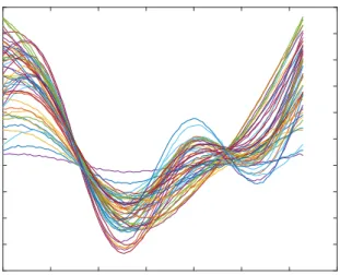
Tecator data. The data are recorded on a Tecator Infratec Food and Feed Analyzer working in the wavelength range 850 - 1050nm by the Near Infrared Transmission (NIT) principle. Each sample contains one of 215 finely chopped pure meat with different moisture, fat and protein contents. For each meat sample the data consists of a 100 channel spectrum of absorbances and the contents of water, fat and protein. The absorbance is -log10 of the transmittance measured by the spectrometer. The spectrometric curves are shown in Figure 2. The sample correlations between fat and water and between fat and protein are -0.9881 and -0.8609, respectively, and that between water and protein is 0.8145. The task is to predict the three contents from the spectrometric curves.
As the spectrometric curves are smooth, the semi-metric based on derivative of order two is adopted in our model. To compare the performance, leave-one-out cross validation is performed, that is, each of the 215 samples is left as test data whilst the remaining data are used for model training. The predicted values are then compared with the measured and the root mean square errors by the proposed Multi-GP with functional covariate and the independent models with functional covariate (Ind-GP)
Wavelengths 850 900 950 1000 1050 Absorbances 2 2.5 3 3.5 4 4.5 5 5.5 6
Figure 2: A graphical display of spectrometric curves. Table 2: The RMSEs for the Tecator data
Fat Water Protein Multi-GP 1.429 1.548 0.942
Ind-GP 1.450 1.816 0.923
GP-MV 1.724 1.516 1.222
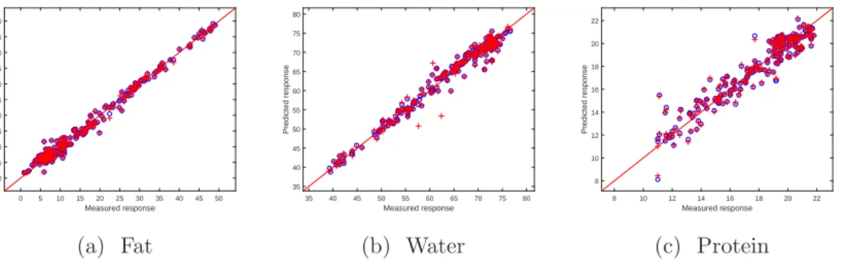
are reported in Table 2. The predictions by both methods are illustrated in Figure 3. Although many functional data can not be analysed by multivariate statistical methods as pointed out earlier, it is, nevertheless, possible to treat the spectrometric curves as multivariate in this example. Therefore, for demonstration we also compare the performance of GPR with functional covariate with that of the conventional GPR with multivariate covariates (GP-MV) where each response is independently modelled by a GPR with the covariates being the absorbances at each wavelength. Since the number of wavelengths is large (100 in total), the usual strategy of PCA is adopted to reduce the number of covariates and five principal components, which account for 99.996% of the total variation, is used in the GPR models as the covariates. The
Measured response 0 5 10 15 20 25 30 35 40 45 50 Predicted response 0 5 10 15 20 25 30 35 40 45 50 (a) Fat Measured response 35 40 45 50 55 60 65 70 75 80 Predicted response 35 40 45 50 55 60 65 70 75 80 (b) Water Measured response 8 10 12 14 16 18 20 22 Predicted response 8 10 12 14 16 18 20 22 (c) Protein
Figure 3: Prediction by leave-one-out cross validation for Tecator data. ’o’: by Multi-GP; ’+’: by Ind-GP.
RMSEs of the predictions by this model are also shown in Table 2 as GP-MV.
It can be seen that, in comparison with the independent model, the Multi-GP method significantly improves the prediction accuracy for water whilst there is marginal improvement for fat. The prediction for protein by Multi-GP is slightly worse than Ind-GP, but in overall terms the former outperforms the independent model. Although GP-MV provides the best prediction for water, its performance on fat and protein is notably worse than the other two methods.
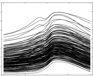
Soil data. This data set was originally studied by [23]. The soil samples were obtained at a long-term field experiment in Abisko, northern Sweden. The samples are from 36 plots, with three subsamples from each plot, giving a total of 108 samples. The wavelength range of 400 - 2500nm (visible and near infrared spectrum) was scanned at 2nm intervals with an NIR spectrophotometer and fluorescence excitation-emission matrices (EEMs) were recorded with a spectrofluorometer. Two reference values, soil organic matter (SOM) was measured as loss on ignition at 550 ◦C, and ergosterol
concentration (EC) was determined through HPLC. The sample correlation between the two reference values is 0.7108.
The semi-metric based on derivative of order two is adopted in our model since the covariate curves are smooth, and the same leave-one-out cross validation experiment
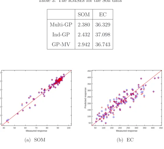
Table 3: The RMSEs for the Soil data SOM EC Multi-GP 2.380 36.329 Ind-GP 2.432 37.098 GP-MV 2.942 36.743 Measured response 40 50 60 70 80 90 100 Predicted response 40 50 60 70 80 90 100 (a) SOM Measured response 50 100 150 200 250 300 350 400 450 Predicted response 50 100 150 200 250 300 350 400 450 (b) EC
Figure 4: Prediction by leave-one-out cross validation for Soil data. ’o’: by Multi-GP; ’+’: by Ind-GP.
as in the previous example is performed. The root mean square errors by Multi-GP, Ind-GP and GP-MV (with five principal components accounting for 99.789% of the total variation) are reported in Table 3, and the predictions by the first two methods are shown in Figure 4.
It can be seen that the proposed Multi-GP model improves the accuracy of predic-tion for both SOM and EC in comparison with the Ind-GP and GP-MV.
The above numerical examples also manifest another advantage of functional data over multivariate, in addition to what has been discussed in the introduction, that is, treating some data as functional rather than multivariate in GPR modelling signifi-cantly reduces the model complexity. For instance, only one parameter is needed for
the spectrometric curves in the soil data, instead of 1050 if each wavelength is treated as a variable or 5-10 if PCA is used to reduce the dimensionality.
4. Conclusion
In this paper we extend the Gaussian process regression models to the situation where the covariates include functional variable as well as multivariate variable and with multidimensional response. The closeness between the functional covariates is measured by the semi-metrics as discussed in [15]. Principal component analysis is performed for the multivariate response and the uncorrelated principal scores are then modelled using Gaussian process regressions. The usefulness of the proposed method over the independent model and the conventional GPR models is demonstrated through some numerical examples.
The proposed Gaussian process model naturally incorporates two different types of covariates: multivariate and functional. And the PCA technique to deal with multi-variate response avoids the widely recognised difficulty in GPR for multiple outputs, that is, to formulate a covariance function that describes not only the correlation be-tween data points, but also the correlation bebe-tween responses. In this paper we assume that the dimension of the response is low so that all the principal components are used in the subsequent regression models. However, if the response is high dimensional and it is intractable to build a GPR model for each of the principal components, we can choose to model fewer number of principal components, for example choosing the minimum number of components which explain at least 95% of the total variation, or, determining this number by cross validation.
Conflict of interest
The authors confirm that there are no known conflicts of interest associated with this publication and there has been no significant financial support for this work that could have influenced its outcome.
Acknowledgement
The authors thank the reviewers for their constructive suggestions and helpful com-ments.
References
[1] A. O’Hagan, Curve fitting and optimal design for prediction, J. Roy. Statist. Soc. Ser. B 40 (1) (1978) 1–42.
[2] D. J. C. MacKay, Introduction to Gaussian processes, Tech. rep., Cambridge Uni-versity (1999).
[3] C. E. Rasmussen, C. K. I. Williams, Gaussian Processes For Machine Learning, The MIT Press, 2006.
[4] T. Chen, J. Morris, E. Martin, Gaussian process regression for multivariate spec-troscopic calibration, Chemometrics and Intelligent Laboratory Systems 87 (2007) 59–67.
[5] K. Wang, T. Chen, R. Lau, Bagging for robust non-linear multivariate calibration of spectroscopy, Chemometrics and Intelligent Laboratory Systems 105 (2011) 1–6. [6] J. Yuan, K. Wang, T. Yu, M. Fang, Reliable multi-objective optimization of high-speed WEDM process based on Gaussian process regression, International Journal of Machine Tools & Manufacture 48 (2008) 47–60.
[7] L. L. T. Chan, Y. Liu, J. Chen, Onlinear system identification with selective recursive Gaussian process models, Industrial & Engineering Chemistry Research 52 (2013) 18276–18286.
[8] Y. Liu, Z. Gao, Real-time property prediction for an industrial rubber-mixing process with probabilistic ensemble Gaussian process regression models, Journal of Applied Polymer Science 132 (6) (2015) 1905–1913.
[9] Y. Liu, C.-P. Chou, J. Chen, J.-Y. Lai, Active learning assisted strategy of con-structing hybrid models in repetitive operations of membrane filtration processes: Using case of mixture of bentonite clay and sodium alginate, Journal of Membrane Science 515 (2016) 245–257.
[10] G. P. Moss, Y. Sun, M. Prapopoulou, N. Davey, R. Adams, W. J. Pugh, M. B. Brown, The application of Gaussian processes in the prediction of percutaneous absorption, Journal of Pharmacy and Pharmacology 61 (9) (2009) 1147–1153. [11] L. T. Lam, Y. Sun, N. Davey, R. Adams, M. Prapopoulou, M. B. Brown, G. P.
Moss, The application of feature selection to the development of Gaussian pro-cess models for percutaneous absorption, Journal of Pharmacy and Pharmacology 62 (6) (2010) 738–749.
[12] D. J. Levitin, R. L. Nuzzo, B. W. Vines, J. Ramsay, Introduction to functional data analysis, Canadian Psychology/Psychologie Canadienne 48 (3) (2007) 135– 155.
[13] J. O. Ramsay, C. J. Dalzell, Some tools for functional data analysis, Journal of the Royal Statistical Society. Series B (Methodological) (1991) 539–572.
[14] J. O. Ramsay, B. W. Silverman, Functional Data Analysis, Springer, New York, 2005.
[15] F. Ferraty, P. Vieu, Nonparametric Functional Data Analysis: Theory and Prac-tice, Springer, New York, 2006.
[16] W. Saeys, B. De Ketelaere, P. Darius, Potential applications of functional data analysis in chemometrics, Journal of Chemometrics 22 (5) (2008) 335–344. [17] A. Aguilera, M. Escabias, M. Valderrama, M. Aguilera-Morillo, Functional
[18] M. Muller, Functional data analysis applied in chemometrics: With focus on NMR nutri-metabolomics, Ph.D. thesis, University of Copenhagen (2015).
[19] P. Boyle, M. Frean, Dependent Gaussian processes, in: Advances in Neural Infor-mation Processing Systems, 2004, pp. 217–224.
[20] B. Wang, T. Chen, Gaussian process regression with multiple response variables, Chemometrics and Intelligent Laboratory Systems 142 (2015) 159–165.
[21] J. Q. Shi, T. Choi, Gaussian process regression analysis for functional data, CRC Press, Boca Raton, FL, 2011.
[22] F. Ferraty, I. Van Keilegom, P. Vieu, On the validity of the bootstrap in non-parametric functional regression, Scandinavian Journal of Statistics 37 (2) (2010) 286–306.
[23] R. Rinnan, A. Rinnan, Application of near infrared reflectance (NIR) and fluores-cence spectroscopy to analysis of microbiological and chemical properties of arctic soil, Soil Biology and Biochemistry 39 (7) (2007) 1664–1673.
List of Figures
1 Sample covariate curves. . . 8 2 A graphical display of spectrometric curves. . . 10 3 Prediction by leave-one-out cross validation for Tecator data. ’o’: by
Multi-GP; ’+’: by Ind-GP. . . 11 4 Prediction by leave-one-out cross validation for Soil data. ’o’: by
Multi-GP; ’+’: by Ind-GP. . . 12
List of Tables
1 The average RMSEs for the simulated data . . . 9 2 The RMSEs for the Tecator data . . . 10 3 The RMSEs for the Soil data . . . 12