Debt Management and Optimal Fiscal Policy with Long Bonds
∗
Elisa Faraglia
a,d, Albert Marcet
b,dand Andrew Scott
c,da University of Cambridge, b Institut d’Anàlisi Econòmica CSIC,
ICREA, UAB and BGSE,
c London Business School, d CEPR
June 2012
Abstract
We study Ramsey optimal fiscal policy under incomplete markets in the case where the government issues long bonds only of maturity N >1. Wefind that many features of optimal policy are sensitive to the introduction of long bonds, in particular tax variability and the long run behavior of debt. When government is indebted it is optimal to respond to an adverse shock by promising to reduce taxes in the distant future as this achieves a cut in the cost of debt financing. Hence, debt management concerns override fiscal policy concerns such as tax smoothing. In the case when the government leaves bonds in the market until maturity wefind two additional reasons why taxes are volatile due to debt management concerns: debt has to be brought to zero in the long run and there are N-period cycles. We formulate our equilibrium recursively applying the Lagrangean approach for recursive contracts. However even with this approach the dimension of the state vector is very large. To overcome this issue we propose a flexible numerical method, the "condensed PEA", which substantially reduces the required state space. This technique has a wide range of applications. To explore issues of policy coordination and commitment we propose an alternative model where monetary and fiscal authorities are independent.
JEL Classification : C63, E43, E62, H63
Keywords : Computational Methods, Debt Management, Fiscal Policy, Government Debt, Maturity Structure, Tax Smoothing, Yield Curve
1
Introduction
As the current European Sovereign Debt crisis reveals taxes, public spending and fiscal deficits all need to take into account funding conditions in the bond market. This makes for a dramatic illustration that debt management should not be subservient tofiscal policy and aimed simply at ∗Marcet is grateful for support from DGES, Monfispol, and Excellence Program of Banco de España. Faraglia and
Scott gratefully acknowledge funding from the ESRC’s World Economy and Finance program. We are grateful to Alex Clymo for research assistance and Gernot Müller and Mikhail Golosov for comments and seminar participants at EEA (Oslo), IAE, UPF, Monfispol. All errors are our own.
minimising the cost of funding debt. A number of recent contributions have studied interactions between debt management and taxation policy in a Ramsey equilibrium setting. Angeletos (2002), Barro (2003), Buera and Nicolini (2004) use models of complete markets whereas Faraglia, Marcet and Scott (2010) argue that optimal fiscal policy and debt management should be studied in an explicitly incomplete market setup. Nosbusch (2008) explores a simplified model of incomplete markets and Lustig, Sleet and Yeltekin (2009) examine an incomplete market model with multiple maturities and nominal bonds. The current paper can be seen as building on these earlier contri-butions. In particular we extend the setup of Aiyagari, Marcet, Sargent and Seppälä (2002), who studied optimal fiscal policy with incomplete markets and short bonds, to the case when bonds mature N periods after having been issued. The motivation for studying longer maturity models comes from Table 1 which shows the average maturity of outstanding government debt for a variety of countries and displays clear differences. Any theory of debt management needs to explain the costs and benefits forfiscal policy of varying the average maturity in this manner. However as this paper documents extending the model to the case of more than one period debt is a non-trivial extension and raises a number of computational, economic and policy assumptions that are either omitted or implicit in the one period case. In this paper we show how to overcome these prob-lems consider a variety of modelling assumptions in order to do so, introduce a new computational method for the efficient solution of models with large steady state and consider the behaviour of optimalfiscal policy and debt management in the presence of long bonds.
INSERT TABLE 1 HERE
The equilibrium in our model of long bonds shows some well known features of standard op-timal fiscal policy under incomplete markets: governments try to smooth taxes, taxes show near-martingale behavior and debt is used as a buffer stock to spread tax increases over all periods after unexpected adverse shocks. However we alsofind that if the government is indebted and an adverse shock occurs the government promises to cut taxes in future periods, when the newly issued long bonds generate a payoff. These future tax cuts "twist" current long interest rates so as to reduce the burden of past debt. This means that a typical debt management concern, i.e reducing the costs of debt, overrides a typical concern of fiscal policy, namely tax smoothing. This promise to cut taxes is the reason that optimal policy is time inconsistent: if the government could, it would renege on the promise to cut taxes. This effect is also present in the one period maturity case but is overwhelmed by an offsetting initial period impact of raising taxes. Only with longer maturities are these two distinct effects disentangled.
A further problem that arises only when dealing with long bonds is what decision to make about outstanding debt at the end of each period. Most of the literature assumes the government buys back each period all previously issued debt and then immediately reissues new bonds. In the case of one period bonds this assumption is innocuous as it is in the case of models with complete markets but it does matter under incomplete markets. As shown in Marchesi (2004) governments rarely buy back outstanding debt before redemption. To quote the UK Debt Management Office (2003) "the UK’s debt management approach is that debt once issued will not be redeemed before maturity."
For this reason we also study optimal policy when the government leaves long bonds in circulation until the time of maturity. We call this the "hold to redemption" case. In this case, at any moment in time the government has a full spectrum of outstanding debt with maturity until redemption ofN, N−1through to 1 year even though the government only ever issuesN period debt. The maturity profile of government debt is therefore much more complex with long bonds and hold to redemption and this will potentially impact debt management and fiscal policy. We find that optimal tax policy is even more volatile in this case: the government promises to cut taxes permanently and there are N−period cycles in tax policy in these models. We also compare our approach with alternative methods that have been proposed which reduce computational complexity. Specifically we compare with the approach of Woodford (2001) and Arellano and Ramanararayanan (2008) who model bonds of different maturities by decaying coupon perpetuities where the decay rates are used to mimic maturity differences. We find important differences between our solutions and those produced by this approach - specifically the interest rate twisting effects that are based around specific maturity dates are absent and instead smoothed out across all periods in the case of decaying coupon perpetuities.
Obtaining numerical simulations is not straightforward. A first difficulty is in obtaining a recursive formulation of the model - to do so we extend the recursive contracts treatment of Aiyagari et al. (2002). A second difficulty arises because the vector of state variables is typically of dimension 2N + 1,hence it grows rapidly with maturity. As many OECD countries issue thirty year bonds, and both France and the UK issue fifty year bonds, this makes for a potentially very large state space. Solving a non-linear dynamic model with these many state variables is not feasible.
To reduce this computational complexity we propose a new method, the "condensed PEA", that reduces the dimensionality of the state vector while allowing, in principle, for arbitrary precision. We show how in the case of a twenty year bond the state space is effectively only four variables. This computational method has wide applicability to other cases beyondfiscal policy and is a major contribution of this paper.
The fact the fiscal authority finds it optimal to twist interest rates to minimise funding costs raises issues of commitment and policy coordination. To assess this we introduce a model where thefiscal authority is separate from the monetary authority setting interest rates. In this way the "twisting" of interest rates is not possible, since the fiscal authority takes interest rates as given. This setup provides a framework to understand the role of commitment in the Ramsey policy, and in the case with buyback it reduces the dimensionality of the state vector as the usual co-state variables of optimal Ramsey policy are no longer present.
In calibrated example allocations we find that interest rates and the persistence of debt are similar across maturities and across the three models of policy considered. The main difference is the long run level of debt, as longer maturities are associated with more debt. Marcet and Scott (2009) (MS)find that incomplete markets with one period bonds better explain the observed persistence of debt than complete market models with one period debt. However the incomplete market model does produce an overshoot of debt and greater persistence than in the data. Both of these charactersitics are better matched with the data when we extend the incomplete market model to the case of long bonds.
The structure of the paper is as follows. Section 2 outlines our main model - a Ramsey model with incomplete markets and long bonds when the government buys back all outstanding debt each period. It also shows properties of the model using analytic results. Section 3 studies numerical issues, introduces the condensed PEA and describes the behavior of the model numerically. Section 4 studies the model of independent powers whilst Section 5 considers the case of hold to redemption whilst a final section concludes.
2
The Model - Analytic Results
Our benchmark model is of a Ramsey policy equilibrium with perfect commitment and coordination of policy authorities in which the government buys back all existing debt each period. In Sections 4 and 5 we relax these assumptions.
The economy produces a single non-storable good with technology
ct+gt≤1−xt, (1) for allt,wherext, ct andgtrepresent leisure, private consumption and government expenditure re-spectively. The exogenous stochastic processgtis the only source of uncertainty. The representative consumer has utility function:
E0 ∞
X t=0
βt{u(ct) +v(xt)} (2) and is endowed with one unit of time that it allocates between leisure and labour and faces a proportional tax rate τt on labor income. The representative firm maximizes profits and both consumers andfirms act competitively by taking prices and taxes as given. Consumers, firms and government all have full information, i.e they observe all shocks up to the current period, and all variables dated t are chosen contingent on histories gt = (gt, ..., g0). All agents have rational expectations.
Agents can only borrow and lend in the form of a zero-coupon, risk-free,N-period bond so that the government budget constraint is:
gt+pN−1,tbN,t−1=τt(1−xt) +pN,tbN,t (3) wherebN,t denotes the number of bonds the government issues at timet. Each bond pays one unit of consumption good inN periods time with complete certainty. The price of an i-period bond at timetispit.In this section we assume that at the end of each period the government buys back the existing stock of debt and then reissues new debt of maturity N,these repurchases are reflected in the left side of the budget constraint (3).In addition government debt has to remain within upper and lower limitsM and M so ruling out Ponzi schmes e.g
M ≤βNbN,t≤M (4) The termβN in this constraint reflects the value of the long bond at steady state so that the limits M , M appropriately refer to the value of debt and are comparable across maturities.1
1Obviously the actual value of debt is p
N,tbN,t,we substitute pN,t by its steady state value βN for simplicity,
We assume after purchasing a long bond the household entertains only two possibilities: one is to resell the government bond in the secondary market in the period immediately after having purchased it, the other possibility is to hold the bond until maturity.2 Letting sN,t be the sales in the secondary market the household’s problem is to choose stochastic processes{ct, xt, sN,t, bN,t}∞t=0 to maximize (2) subject to the sequence of budget constraints:
ct+pN,tbN,t= (1−τt) (1−xt) +pN−1,tsN,t+bN,t−N −sN,t−N+1
with prices and taxes {pN,t, pN−1,t, τt} taken as given. The household also faces debt limits anal-ogous to (4), we assume for simplicity that these limits are less stringent than those faced by the government, so that in equilibrium, the household’s problem always has an interior solution.
The consumer’s first order conditions of optimality are given by vx,t uc,t = 1−τt (5) pN,t = βNEt(uc,t+N) uc,t (6) pN−1,t = βN−1Et(uc,t+N−1) uc,t (7)
2.1
The Ramsey problem
We assume the government has full commitment to implement the best sequence of (possibly time inconsistent) taxes and government debt knowing equilibrium relationships between prices and allocations. Using (5), (6) and (7) to substitute for taxes and consumption the Ramsey equilibrium can be found by solving
max {ct,bN,t} E0 ∞ X t=0 βt{u(ct) +v(xt)} s.t. βN−1Et(uc,t+N−1)bN,t−1=St+βNEt(uc,t+N)bN,t (8) and (4), andxt implicitly defined by (1).
To simplify the algebra we defineSt= (uc,t−vx,t) (ct+gt)−uc,tgt as the “discounted” surplus of the government and set up the Lagrangian
L=E0 ∞ X t=0 βt©u(ct) +v(xt) +λt £ St+βNuc,t+NbN,t−βN−1uc,t+N−1bN,t−1 ¤ +ν1,t ¡ M−βNbN,t ¢ +ν2,t ¡ βNbN,t−M ¢ª
whereλtis the Lagrange multiplier associated with the government budget constraint e.g the excess burden of taxation, and ν1,t and ν2,t are the multipliers associated with the debt limits.
2We need to introduce secondary market saless
The first-order conditions for the planner’s problem with respect toct and bN,t are
uc,t−vx,t+λt(ucc,tct+uc,t+vxx,t(ct+gt)−vx,t) (9) +ucc,t(λt−N −λt−N+1)bN,t−N = 0
Et(uc,t+Nλt+1) =λtEt(uc,t+N) +ν2,t−ν1,t (10) withλ−1=...=λ−N = 0.
These FOC help characterise some features of optimalfiscal policy with long bonds. Following the discussion in Aiyagari et al. (2002) we see that, in the case where debt limits are non binding, (10) implies λt is a risk-adjusted martingale, with risk-adjustment measure Et(uc,tuc,t+N
+N), indicating that the presence of the state variableλin the policy function imparts persistence in the variables of the model. The term
Dt= (λt−N −λt−N+1)bN,t−N
in (9) indicates that a feature of optimalfiscal policy will be that what happened in period t−N has a specific impact on today’s taxes. Since we haveuc,t−vx,t= 0and zero taxes in thefirst best, a high Dt pulls the model away from the first best and zero taxes. If Dt > 0 it can be thought of as introducing a higher distortion in a given period. In periods when gt−N+1 is very high we have that the cost of the budget constraint is high soλt−N+1 is high, and if the government is in debt Dt <0 so that taxes should go down att. Of course this is not a tight argument, as λt also responds to the shocks that have happened between t and t−N and λt also plays a role in (9), but this argument is at the core of the interest rate twisting policy we identify below. In order to build up intuition for the role of commitment and to provide a tighter argument, we now show two examples that can be solved analytically.
2.2
A model without uncertainty
Assume for now that government spending is constant, gt = g and the government is initally in debt such that bN−1 >0. In this case the long bonds complete the market so that the only budget constraint of the government is :
∞ X t=0 βtuc,t uc,0 e St = bN,−1 pN0−1, or ∞ X t=0 βt St = bN,−1 βN−1uc,N−1 (11) whereSet= uc,tSt is the “non-discounted” surplus of the government. This shows that for a given set of surpluses the funding costs of initial debt bN−1 >0 can be reduced by manipulating consumption such that ct < cN−1 for allt 6=N.As long as the elasticity of consumption with respect to wages is positive, as occurs with most utility functions, this will be achieved by promising a tax cut in periodN−1 relative to other periods e.g
τt = τ for all t6=N−1 (12) τ > τN−1
This promise achieves a reduction ofuc,N−1,reducing the cost of outstanding debt. In other words, the long end of the yield curve needs to be twisted up.3 Interestingly, even though there are no
fluctuations in the economy, (12) shows that optimal policy implies that the government desires to introduce variability in taxes. In other words, optimal policy violates tax smoothing.This policy is clearly time inconsistent - if the government were able to reoptimize by surprise at some period t0 >0, t0 < N it will instead then promise a cut in taxes in period t0+N−1.
2.3
A model with uncertainty at
t
= 1
The previous subsection abstracted from uncertainty. We now introduce uncertainty into our model. In the interest of obtaining analytic results we assume uncertainty occurs only in the first period, ieg is given by4: ½
gt=g fort= 0and t≥2 g1 ∼Fg
for some non-degenerate distributionFg.Since future consumption andλ’s are known the martin-gale condition impliesuc,t+Nλt+1 =λtuc,t+N and
λt=λ1 t >1
It is clear that in the case of short bonds (N = 1) equilibrium implies ct and τt constant for t≥2, reflecting the fact that even though markets are incomplete the government smooths taxes after the shock is realized.
For the case of long bonds when N >1,the FOC with respect to consumption (9) is satisfied forDt= (λt−N −λt−N+1)bN,t−N
Dt= 0 fort≥0 and t6=N −1, N (13)
DN−1 =λ0bN,−1 , DN = (λ0−λ1)bN,0 (14)
Hence equilibrium satisfies
ct= c∗(g1) fort≥2and t6=N, N−1 (15) for a certain functionc∗ i.e consumption is the same in all periodst≥2andt6=N, N−1,although this level of constant consumption depends on the realization of the shock g1. Clearly, cN−1, cN also depend on the realization ofg1.
In this model, when the shock g1 is realised the government optimally spreads out the taxation cost of this shock over current and future periods. Typically the government gets in debt in period 1 ifg1 is high, so all future taxes fort≥2are higher and future consumption lower. This would also happen with short bondsN = 1.What is new with long bonds is that optimal policy introduces tax volatility, since taxes vary in periods N −1 and N, even though by the time the economy arrives at these periods no more shocks have occured for a long time.
3
This is, of course, a manifestation of the standard interest rate manipulation already noted by Lucas and Stokey (1983), except that in our case the twisting occurs inN periods.
4
2.3.1 An Analytic Example
To make this argument precise consider the utility function c1−γc t 1−γc −B (1−xt)1+γl 1 +γl (16) forγc, γl, B >0.
Result 1 Assume utility (16) and bN,−1>0. For a sufficiently high realization of g1 we have
τ1 = τt for allt≥1, t6=N−1, N τ1 > τN−1, τN
The inequalities are reversed if bN,−1 <0 or if the realization of g1 is sufficiently low. Proof
Since λt=λ1 t >1 the FOC of optimality yield uc,t vx,t − B+ (γl+ 1)λ1 (1 + (−γc+ 1)λ1)B + (λt−N −λt−N+1)Ft= 0 fort≥1 whereFt≡ (1+(ucc,tbN,t−γ −N c+1)λ1)B.
Consider t= 1.For any long maturity N >1 we have that λt−N =λt−N+1 = 0when t= 1so that uc,1 vx,1 = B+ (γl+ 1)λ1 (1 + (−γc+ 1)λ1)B (17) Therefore we can write
uc,t vx,t −
uc,1 vx,1
= (λt−N+1−λt−N)Ft= 0 for t≥1 (18)
That τt=τ1 for all t >1and t6=N−1, N follows from (15).
Now we show thatFt<0fort=N−1, N.Sinceλ1, B, γl>0we have thatB+ (γl+ 1)λ1 >0. Since uc,1, vx,1 > 0 clearly (17) implies that (1 + (−γc+ 1)λ1)B > 0. Since we consider the case of initial government debt bN,−1 >0 this leads to bN,0 >0 and since ucc,1 <0 we have Ft <0for t=N−1, N.
Since for t=N −1we have λt−N −λt−N+1=−λ0<0it follows uc,N−1
vx,N−1
< uc,1 vx,1 ⇒
τN−1< τtfor all t >1, t6=N−1, N.
Also, it is clear from (17) that high g1 implies a high λ1. Since the martingale condition implies Et(uc,Nλ1) =λ0E0(uc,N) for slightly high g1 we have λ1 > λ0 Therefore, for t=N and ifg1 was high enough we have λt−N−λt−N+1=λ0−λ1 <0so that (18) implies
uc,N vx,N ,uc,N−1 vx,N−1 < uc,1 vx,1 ⇒ τN, τN−1 < τ1 ¥
Intuitively, in period t=N−1 there is a tax cut for the same reasons as in Section 2.2. New in this section is the tax cut (for highg1)att=N.The intuition for this is clear: when an adverse shock to spending occurs att= 1the government uses debt as a buffer stock sobN,1 > bN,0, as this allows tax smoothing by financing part of the adverse shock with higher future taxes. But since future surpluses are higher than expected as the higher interest has to be serviced, the government can lower the cost of existing debt by announcing a tax cut in period N,since this will reduce the price pN−1,0 of periodt= 1 outstanding bonds bN,0. The tax cut at t=N is a stochastic analog of the tax cut described in section 2.2.
2.3.2 Contradicting Tax Smoothing
The above result shows that in this model tax policy is subordinate to debt management. In models of optimal policy the government usually desires to smooth taxes. Taxes would be constant in the above model if the government had access to complete markets. But wefind that the government increases tax volatility in period N, long after the economy has received any shock. Therefore, government forfeits tax smoothing in order to enhance a typical debt management concern, namely reducing the average cost of debt. Obviously this policy is time inconsistent: if the government could unexpectedly reoptimize in periodt= 2given its debtbN,1it would renege on the promise to cut taxes in periodN,instead it would promise to lower taxes in periodN+ 1. It is clear from this discussion that what will matter for the policy function is the termDN = (λ0−λ1)bN,0.Therefore it is the interaction between past λ’s and pastb’s that determines the size and the sign of today’s tax cut. A linear approximation to the policy function would fail to capture this feature of the model and it would be quite inaccurate.
To summarize, we have proved that in the presence of an adverse shock to spending the gov-ernment has to take three actions: i) increase taxes permanently, ii) increase debt, iii) announce a tax cut when the outstanding debt matures. Effects i) and ii) are well known in the literature of optimal taxation under incomplete markets, effect iii) is clearly seen in this model with long bonds since the promise is madeN periods ahead. Obviously in the case of short maturityN = 1 of Aiyagari et al. the effect ofD1 would be felt in deciding optimallyτ1 but would be confounded with the fact g1 is stochastic making iii) harder to see in a model with short bonds.
3
Optimal Policy - Simulation Results
We now turn to the case where gt is stochastic in all periods. As is well known analytic solutions for this type of model are infeasible so we utilise numerical results. The objective is to compute a stochastic process {ct, λt, bN,t} that solves the FOC of the Ramsey planner, namely (8), (9) and (10). First we obtain a recursive formulation that makes computation possible, then we describe a method for reducing the dimensionality of the state space andfinally we discuss the behaviour of the economy.
3.1
Recursive Formulation
Using the recursive contract approach of Marcet and Marimon (2011) the Lagrangean can be rewritten as : L=E0 ∞ X t=0 βt{u(ct) +v(xt) +λtSt+uc,t(λt−N−λt−N+1)bN,t−N (19) +ν1,t ¡ M−βNbN,t ¢ +ν2,t ¡ βNbN,t−M ¢ª forλ−1 =...=λ−N = 0.
Assuminggtis a Markov process, as suggested by the form of this Lagrangean, Corollary 3.1 in Marcet and Marimon (2011) implies the solution satisfies the recursive structure5
⎡ ⎣ bN,t λt ct ⎤ ⎦ = F(gt, λt−1, ..., λt−N, bN,t−1, ..., bN,t−N) λ−1 = ...=λ−N = 0, given bN,−1
for a time-invariant policy function F. This allows for a simpler recursive formulation than the promised utility approach, as the co-state variablesλdo not have to be restricted to belong to the set of feasible continuation variables. The state vector in this recursive formulation has dimension 2N + 1.
3.2
The Condensed PEA
It is relatively easy to obtain solutions of large dimensional dynamic stochastic models using linear approximations to the policy functionF. These approximations are quite accurate for many models of interest but are often ill suited to incomplete market models offiscal policy. In our model the debt limits occassionally bind for debt levels similar to those observed in the real world. When debt limits occassionally bind the derivative ofF near the debt limit may be quite different from the derivative near steady state so that a linear approximation is likely to be inaccurate. Furthermore, per our discusion in Section 2.1, it is clear that what determines the effect of previous commitments on today’s tax is the term Dt= (λt−N −λt−N+1)bN,t−N. In other words it is the interaction between past λand bN.A linear approximation to the policy function would fail to capture this feature of the model and so would miss key aspects of optimal policy under full commitment6. To overcome this difficulty we introduce a solution method based on the Parameterized Expectation Algorithm
5
In this model it is possible to reduce the state space even further by recognising that the only relevant state variables areN lags ofst=bN,t(λt−λt−1).We do not exploit this feature of the model as it is very specific to this
version of the model. For example, the no buyback case of section 5 needs all state variables. 6
In this particular model it might be enough to includeDt as a state variable instead of pastλ’s and pastbN’s.
But this discussion highlights that non-linear terms are important for optimalfiscal policy. Even though a "trick" can be found for this particular model where a linear approximation may work a different trick would be needed, or may not be available, for another model. A general technique that avoids having to find these tricks is to use an algorithm that can capture these non-linearities.
of den Haan and Marcet (1990). This allows us to reduce the dimensionality of the policy function actually solved for while keeping an accurate solution. Using PEA is useful because it does capture the relevant non-linearities described in Section 2.3 even if the expectations are parameterized as linear functions and because it allows for a natural space reduction method that we call "condensed PEA".
This method goes as follows. Denote the state vector asXt= (gt, λt−1, ..., λt−N, bN,t−1, ..., bN,t−N). The idea is that even though theoretically all elements ofXt are necessary in determining decision variables at t, it is unlikely that in the steady state distribution each and everyone of these vari-ables plays a substantial role in determining the solution. For us, most likely some function of these lags will be sufficient to summarize the features from the past that need to be remembered by the government in order to take an optimal decision. In the context of PEA this can be expressed in the following way.
One of the expectations requiring approximation is
Et{uc,t+N} (20) appearing in (10). This expectation is a function, in principle, of all elements inXt,but it is likely that in practice a few linear combinations ofXt may be sufficient to predictuc,t+N .There are two reasons for this. First, the very structure of the model suggests that elements ofXtare very highly correlated with each other, suggesting that a few linear combinations ofXthave as much predictive power as the whole vector. Another way of saying this is that it is enough to project any variable on the principal components of Xt. Other methods available for reducing the dimensionality of state vectors have emphasized this aspect. The second reason is that some principal components of Xt may be irrelevant in predictinguc,t+N in equilibrium and, therefore, they can be left out of the approximated conditional expectation. So the goal is to include only linear combinations ofXt that have some predictive power for uc,t+N,the remaining linear combinations can be understood as appearing in the conditional expectation with a coefficient of zero.
More precisely, we partition the state vector into two parts: a subset of n state variables
{Xcore
t } ⊂{Xt}, where n < 2N + 1 is small and an omitted subset of state variables ©
Xout t
ª =
{Xt}−{Xtcore} of dimension 1 + 2N −n. We first solve the model including only Xtcore in the parameterized expectations. If the errorφt+N ≡uc,t+N −Et{uc,t+N} found using just these core variables is unpredictable withXout
t we would claim the solution with core variables is the correct one. IfXtout can predict this error we thenfind the linear combination ofXtout that has the highest predictive power for φt+N. We add this linear combination to the set of state variables, solve the model again with this sole additional state variable, check if Xout can predictφ
t+N and so on. Formally, given the set of core variables we define the condensed PEA as follows.7,8
Step 1 Parameterize the expectation as
Et{uc,t+N}= (1, Xtcore)·β1 (21)
7
This definition assumes we are interested in the steady state distribution, of course it could be modified in the usual way to take into account transitions.
8
For convenience we describe these steps with reference only to the expectation Et{uc,t+N}. In practice the
expectationsEt{uc,t+Nλt+1}andEt{uc,t+N−1}appearing in the FOC also need to be parameterized concurrently
Find values for β1 ∈ Rn+1 , denoted β1,f, that satisfy the usual PEA fixed point i.e where the series generated by(1, Xcore
t )·β1,f causes this to be the best parameterized expectation. This solution is of course based on a restricted set of state variables. It is therefore necessary to check if the omission ofXoutaffects the approximate solution. The next step orthogonalizes the information inXtout,this will be helpful to arrive at a well conditionedfixed point problem in Step 4.
Step 2 Using a long run simulation run a regression of each element ofXtout on the core variables. LetXi,tout be the i−th element, we run the regression
Xi,tout= (1, Xtcore)·b1i +u1i,t b1i ∈R2N+2−n and calculate the residuals
Xi,tres,1 =Xi,tout−(1, Xtcore)·b1i. (22) It is clear thatXres,1adds the same information toXcoreasXout, butXres,1has the advantage that it is orthogonal toXcore.
Step 3 Using a long run simulationfind α1∈Rn+1 such that
α1 = arg min α T X t=1 ³ uc,t+N −Xtcore·β1−X res,1 t ·α ´2 (23)
Ifα1 is close to zero the solution with onlyXcoreis sufficiently accurate and we can stop here. Otherwise go to
Step 4 Apply PEA addingXtres,1·α1 as a state variable, ie parameterizing the conditional expec-tation as Et{uc,t+N}= ³ Xtcore, Xtres,1α1 ´ ·β2
where β2 ∈Rn+2. Find afixed point β2,f for this parameterized expectation. Since β1,f is a fixed point, sinceXtcore and Xtres,1 are orthogonal and since the linear combinationα1 has high predictive power it makes sense to use as initial condition for the iterations of the fixed point β2,f (n+2)×1 = µ β1,f 1 
Go to Step 2 with³Xcore t , α1X
res,1
t ´
in the role of Xcore
t ,find a new linear combination, etc.
A couple of remarks end this subsection. In the presence of many state variables it has been customary in dynamic economic models to try each state variable in order. The idea is to add state variables one by one until the next variable does not change much the solution found. For example, if many lags are needed we add the first lag, then the second lag, and so on. If at some
step the solution changes very little it is claimed that the solution is sufficiently accurate. But it is easy to find reasons why this argument may fail. For instance, maybe the variables further down the list is more relevant.9 This is the case, by the way, in our model, where state variable λt−N and bN,t−N play a key role in determining the solution at t. Or it can be that all the remaining variables together make a difference but they do not make a difference one by one. Our method gives a chance to all these variables to make a difference in the solution, therefore it is more efficient infinding relevant state variables, as Step 3 indicates automatically if they are needed and which of them are to be introduced.
The whole argument in this section is made for linear conditional expectations, as in (21). Of course the same idea works for higher-order terms. In order to check the accuracy for higher order terms one can use the condensed PEA with higher-order polynomial terms, i.e one can check if linear combinations of, say, quadratic and cubic terms of Xt have predictive power in Step 2, include these inXtout and go through Steps 2 to 4 above.
The variables included in Xtcore are not the only ones influencing the solution. Due to the nature of PEA past variables can have an effect even if they are excluded from the parameterized expectation. For example, even if wefind a solution Xtcore= (λt−1, bN,t−1, gt) that excludes λt−N and bN,t−N from the parameterized expectation these state variables will influence the solution at tthrough their presence in (9).
3.3
Solving the Model with Condensed PEA
The utility function (16) was convenient for obtaining the analytic results of Section 2.3. In this section however we use a utility function more commonly used in DSGE models:
c1−γ1 t 1−γ1 +η x1−γ2 t 1−γ2
We choose β = 0.98, γ1 = 1 and γ2 = 2. We set η such that if the government’s deficit equals zero in the non stochastic steady state agents work a fraction of leisure equal to 30% of their time endowment.
For the stochastic shock gwe assume the following truncated AR(1) process:
gt= ⎧ ⎨ ⎩ g if (1−ρ)g∗+ρgt−1+εt> g g if (1−ρ)g∗+ρgt−1+εt< g (1−ρ)g∗+ρgt−1+εt otherwise
We assume εt∼N(0,1.44)2, g∗ = 25, with an upper bound g equal to35% and a lower bound g= 15% of average GDP andρ= 0.95. M is set equal to90% of average GDP andM =−M .
9
For another example, incomplete market models with a large number of agents need as state variable all the moments of the distribution of agents, which is an infinite number of state variables. Usually these models are solved
first by using thefirst moment as a state variable, and checking that if the second moment is added nothing much changes. But it could be, of course, that the third or fourth moment are the relevant ones, specially since the actual distribution of wealth is so skewed.
We choose Xtcore= (λt−1, bN,t−1, gt) henceXtout = (bN,t−2, ..., bN,t−N, λt−2, ..., λt−N). To test if sufficient variables are included for an accurate solution in Step 3 we use as our tolerance statistic:
dist= R
2
aug−R2 R2
where R2 and R2aug denote the goodness of fit of the original regression based on the condensed PEA and augmented with the linear combination of residuals respectively. We use for tolerance criterion dist ≤ 0.0001. Table 2 summarizes the number of linear combinations needed for each maturity whilst Table 3 gives details and shows the number of linear combinations needed for each approximations and the R2 anddist.
The advantages of the condensed PEA are readily apparent. In nearly half the cases the core variables are sufficient to solve the model and at most only one linear combination of omitted variables required to improve accuracy. Clearly the condensed PEA can be used to solve models with large state spaces with relatively small computational cost, since the state vector is in principle of dimension 41 but utilising a dimension of 4 is sufficient . Whilst we have focused on a case of optimalfiscal policy and debt management this methodology clearly has much broader applicability
HERE TABLES 2 AND 3
3.4
Optimal Policy - The Impact of Maturity
3.4.1 Interest Rate Twisting
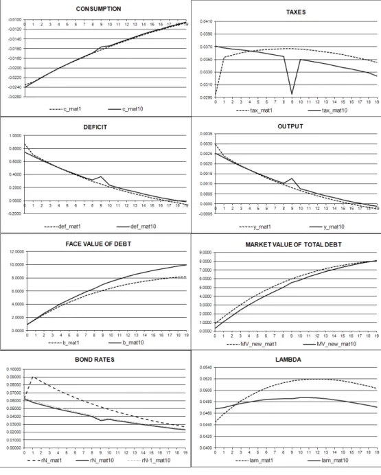
Figures 1 and 2 display the impulse response functions of key variables to an unexpected shock in gt. The solution is computed using the condensed PEA10. The vertical axis is in units of each of the variables and expresses deviations from the value that would occur for the given initial condition ifgt=gss.
Figure 1 is for the case when the government has zero debt on impact. The only significant differences across maturity are on the face value of debt and interest rates. But these differences are immaterial : the face value of debtbN,tis obviously higher forlong bonds, as long debt is discounted more heavily so its face value needs to be higher. What is relevant is the market value of debt, which is similar. As usual in endowment models the long interest rates respond less to shocks than the short interest rate. As usual in models of incomplete markets it is optimal to use debt as a buffer stock so that debt displays considerable persistence.
HERE FIGURE 1
Figure 2 shows the same impulse response functions but in this case we assume the government is indebted on impact such thatbN,t−1 = 0.5y∗/βN wherey∗ is steady state output.
1 0Since debt is very persistent, to ensure we visit all possible realizations in the long run simulations of PEA we initialize the model at 9 different initial conditions, simulate it for 5000 periods for each initial condition, doing this 1000 times per initial condition, and compute conditional expectations discarding thefirst 500 observations for each simulation.
HERE FIGURE 2
With long bonds of maturity N = 10 there is a blip in taxes at the time of maturity of the outstanding bonds. This is a reflection of the promise to cut taxes with the aim to twist interest rates, as discussed in Section 2.3, only now the interest rate twisting occurs each period there is an adverse shock if the government is in debt. The size of the promised tax cut depends on how much larger is today’s shock relative to yesterday’s shock (λt−1−λt) and the level of today’s debt.
3.4.2 Optimal Policy with Short Bonds
This discussion helps to understand the role of commitment in the model of short term bonds as in Aiyagari et al (2002). Consider the case when the government is indebted when an adverse shock occurs, as in Figure 2. As we explained in Section 2.3 optimal policy is to increase current taxes but promise a tax cut in N −1 periods. In the case of long bonds the promised tax cut is clearly distinct from the current increase in taxes. But in the case of short bonds N = 1 the two effects are confounded as they happen in the same period.
This is clearly seen in the response of taxes depicted in Figure 3 for maturities N = 1,5,10,20. Given our previous discussion it is clear why the blip in taxes keeps moving to the left as we decrease the maturity until the blip simply reduces the reaction of taxes on impact at N = 1. Therefore optimal policy for short bonds is to increase taxes on impact but less than would be done if considerations of interest rate twisting were absent or if the debt were zero.
Figure 3 also shows that In the case when the government has assets the blip in taxes goes upwards, as the government desires to increase the value of assets. It is clear that for short bonds the increase in taxes on impact if the govenment initially has assets is much larger than if the government is indebted.
HERE FIGURES 3 3.4.3 Second Moments
Table 4 shows second moments for the economy at steady state distribution for different maturi-ties11. With the exception of debt and deficit all the moments differ only to the second or third decimal place across maturities. This may be surprising, as we have seen that tax policy does change with maturity and since we know that under incomplete markets the way government fi -nances its expenditure can affect the real economy. However with the government only issuing one type of bond in each case tax smoothing is mainly achieved by using debt as a buffer stock rather than throughfiscal insurance (defined in Faraglia Marcet and Scott (2008) as achieving variations in the market value of debt which offset adverse expenditure or tax shocks). Thefluctuations of all variables are driven mostly by the strong low frequency fluctuations of debt, so that the interest rate twisting plays relatively little role in these steady state second moments. We return to this issue later in the discussion of Figure 6.
1 1
These moments have been computed from very long simulations using the approximate policy function computed as described before.
The main exception are the levels of debt and deficit : government in the long run holds assets, but average asset holding are lower for higher maturities. The mean of assets at steady state for 20 year bonds is half the average assets compared for short bonds, due to the different opportunities forfiscal insurance that are offered by long bonds.
As is well known, in models of optimal policy with incomplete markets, there is a force pushing the government to accumulate long bonds in the long run. More precisely, extending the results in Aiyagari et al (2002) Section III one can easily prove that in the case of linear utility (u(c) =c) the government would purchase a very large amount of private long bonds in the long run, enough to abolish taxes. This accounts for the negative means for debt shown in Table4. On the other hand, as argued in Angeletos (2002), Buera and Nicolini (2004) and Nosbusch (2008), if the term premium is negatively correlated with deficits (as it is in our model) it is optimal for the government toissue long bonds, as this provides fiscal insurance. Hence the government is aware that accumulating a very large amount of privately issued long bonds increases the volatility of taxes. This force accounts for thelower asset accumulation withlonger maturities shown in Table 4.
HERE TABLE 4
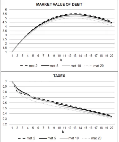
Varying the average maturity of debt also has an influence on the persistence of debt. Marcet and Scott (2009) show that measures of relative persistence are a good way of assessing the extent of market incompleteness and so Figure 4 shows for various variables the measure :
Pyk = V ar(yt−yt−k) kV ar(yt−yt−1)
.
HERE FIGURE 4
The closer to 0 this measure the less persistence the variable shows, whereas the closer to 1 the measure the more the variable shows unit root persistence. Marcet and Scott (2009) showthat observed k variances for US debt were even higher than 1, for examplePDebt10 ≈2.5 (see Figure 2 in MS). Values ofPk
Debt higher than one are incompatible with complete market models and optimal policy, but they easily arise under incomplete markets. However MS also report a shortcoming of incomplete markets : debt display too much persistence under incomplete markets, as they report P10
Debt= 10 (see Figure 6 in MS).
Figure 4 shows the small sample mean of persistence measures for our model when the govern-ment is initially in debt12. NowPDebt10 = 4.1for 20 year bonds so the gap between the data and the model is now one fifth of the gap reported by MS. This improvement is in part due to our use of small sample moments, while MS reported k-variance ratios at steady state distribution. Note that even for a short maturity of N=2 (and als for N=1, not reported in Figure 4) we have PDebt10 ≈5, nearly cutting the persistence in half relative to MS.
1 2The small sample means are found by fixing initial bonds at a level of debt equal to 0.5y*, obtain simulations of 50 periods, computePk
y for each realisation and averagePyk over many realisations all starting at the same initial
3.5
Modelling Maturity With Decaying Coupon Perpetuities
In order to overcome the problem of dimensionality some authors model long bonds as perpetuities with decaying coupon payments where the rates of decay mimic differences in maturity (e.g Wood-ford (2001), Broner, Lorenzoni and Schmulker (2007), Arellano and Ramanarayanan (2008)). In this formulation the government issues perpetuities with coupon payments that decay geometrically i.e a bond with decay factorδLpays a coupon equal toδjLcpj in periodj.The decay rate determines the effective maturity of the bond as the bond’s duration is defined by1/(1−δL) so that a bond of effective maturity 10 years has δL = 0.1. In this case total payments from all previously and currently issued perpetuities are then given byT Pt=cpt+δLcpt−1+δ2Lcpt−2+...+δtLcp0 which follows the recursive structure T Pt = δLT Pt−1 +cpt. Treating this as the outstanding stock of the perpertuity we have a convenient way of dealing with long maturity bonds which dramatically reduces the state space as it is only necessary to keep track of the total number of bonds issued and not the number of bonds issued in each period. This reduction in the state space means that the condensed PEA is no longer required and the model can be solved using more conventional methods.
Whilst assuming decaying coupon payments has great computational merit it is not without modelling consequences. One justification for assuming decaying payoffs is that it mimics a bond portfolio withfixed shares that decay with maturity. However since our goal is to build a model of debt management where the object is precisely to study the appropriate portfolio weights, assuming
fixed portfolio weights would be inappropriate. Further although modelling bond payoffs in this way would yield smaller state space vectors it is contrary to the structure of most government portfolios where most of the payoffoccurs at the time of maturity, as in this model, whereas with decaying coupons the majority of cash flow is paid out in the early years.
INSERT FIGURE 5
Further assuming decaying coupons also leads to different solution paths to the ones we have explained above. Figure 5 shows the impulse response functions of tax rates in response to a government expenditure shock for the case of a one year bond, a ten year bond (as above and solved for using the condensed PEA) and a bond with decaying coupons with duration set equal to 10 under the case of no debt, positive initial debt and a government that inherits a positive asset position. Focusing on the case with zero initial debt, in which case the government has no incentive to engage in interest rate twisting, we see taxes follow the same smooth path across all three models however whilst with the one and ten year bonds taxes follow a risk adjusted martingale that sees them slowly declining over time, for the case of decaying coupons we have taxes smoothly trending upwards. The more revealing differences are shown for the case where government debt is not initially zero. In the case where the government inherits positive debt it uses taxes to twist interest rates to reduce funding costs in the manner described above. However with decaying coupons taxes now decline smoothly across all periods. The logic is simple as now with decaying coupons the government has incentive to "twist" every period and so taxes fall smoothly each period as the interest rate twisting incentive occurs every period.
4
Independent Powers
In Sections 2 and 3 we found that full commitment implied a tight connection between interest rate policy, debt management and tax policy: when government is in debt and spending is high the government promises a tax cut inN−1periods, knowing that this will increase future consumption and this increases long interest rates in the current period. The reader may think that this optimal policy is not relevant for the "real world" for at least two reasons. First, different authorities influence interest rates andfiscal policy, it is unlikely that they will coordinate in the way described before and, secondly, it is unlikely that governments can commit to a tax cut in the distant future and actually carry through with the promise. Some papers in the literature react to this type of criticisms by writing down models where government policy is discretionary. But assuming that the government has no possibility of committing is also problematic, as governments frequently do things for the very reason they have previously committed to do so.
For these reasons in this section we change the way policy is decided in this model. We relax the assumption of perfect coordination and assume the presence of a third agent, a monetary authority that fixes interest rates in every period. The fiscal authority now takes interest rates as a given and implements optimal policy given these interest rates. We examine an equilibrium where the two policy makers play a dynamic Markov Nash equilibrium with respect to the strategy of the other policy power and they both play Stackelberg leaders with respect to the consumer. More precisely, thefiscal authority chooses taxes and debt given a sequence for interest rates, the monetary authority simply chooses interest rates that clear the market and the fiscal authority maximizes the utility of agents. This assumption sidesteps the issues of commitment, now there is no room for interest rate twisting on the part of thefiscal authority.
It is easy to think of models where even if the monetary authority is independent it can not deviate too much from equilibrium interest rates of the flexible price model. Therefore we take a limit case and assume that the monetary authority simply sets in equilibrium interest rates as:
pN,t = βNEt(uc,t+N) uc,t (24) pN−1,t = βN−1Et(uc,t+N−1) uc,t .
given agents’ consumption. To solve this model we are looking for an interest rate policy function
R:R2 →R2 such that if long interest rates att are given by
(p−N,t1, p−N,t1−1) =R(gt, bN,t−1) (25) then (24) holds with thefiscal authority maximizing consumer utility in the knowledge of all market equilibrium conditions but taking the stochastic process for interest rates as given it chooses a bond policy such that (25) holds.
From the point of view of the fiscal authority the problem now is a standard dynamic pro-gramming problem such that the vector of state variables is now (bN,t−1, gt).An advantage of this model is there is no longer any reason for longer lags to enter the state vector, as past Lagrange
multipliers do not play a role. Therefore this separation of powers approach is an alternative way to reducing the state space and simplifying the solution of the model.
In this case of independent powers the Lagrangian of the Ramsey planner becomes L=E0 ∞ X t=0 βt{u(ct) +v(xt) +λt[St+pN,tbN,t−pN,t−1bN,t−1] (26) +ν1,t ¡ M−βNbN,t ¢ +ν2,t ¡ βNbN,t−M ¢ª
The first order condition with respect to consumption is
uc,t−vx,t+λt(ucc,tct+uc,t+vxx,t(ct+gt)−vx,t) +ucc,tλt(pN,tbN,t−pN−1,tbN,t−1) = 0 and using the government’s budget constraint gives
uc,t−vx,t+λt(ucc,tct+uc,t+vxx,t(ct+gt)−vx,t) +ucc,tλt µ gt− µ 1−vx,t uc,t ¶ (1−xt) ¶ = 0 (27) To see the impact of Independent Powers we calibrate the model as in Section 3 and consider the caseN = 10.Figure 6 compares the impulse responses to a one standard deviation shock to the innovation in the level of government spending (in the presence of government debt) between inde-pendent powers and the benchmark model of Section 3. As can be seen the model of indeinde-pendent powers does not show the blip in taxes at maturity. In this case debt management is subservient to tax smoothing and is aimed at lowering the variance of deficits.
HERE FIGURE 6
To better understand the magnitude of the interest twisting channel we can compare our in-dependent powers model with our earlier benchmark model. We simulated the models at different time horizons T = 40, T = 200and T = 5000discarding thefirst 500 periods. We calculated the standard deviation of taxes for each realizations and averaged across simulations. We repeat the same exercise for N = 2,5,10,15,20. Figure 7 shows the results.
HERE FIGURE 7
In shorter sample periods the effect of twisting interest rates in connection with initial period debt is significant and provides a higher level of tax volatility in the benchmark model. Naturally ss we increase the sample size the initial period effect diminishes.
The second moments of the model in this section are shown in Table 5. They are extremely similar to those of the benchmark model in Table 4. We have essentially a very similar amount of bond issuance, debt persistence, tax smoothing etc, the only difference being that the interest rate twisting adds some tax volatility, but this volatility only shows up in second moments with short samples as shown in Figure 6. We conclude that the model of independent powers may be a good model to have in the toolkit as it retains many of the interesting features of the Ramsey models, it has the same steady state moments, it avoids the technicalities arising from the very large state vector and it avoids discussion on the role to commitment at very long horizons. There are, however, issues of tax volatility showing up in small samples where the two models differ.
5
Hold to Redemption
With long bonds the government has a choice to make at the end of every period. It can buy back the N period bonds issued last period, as assumed in Sections 2 and 3 and then sell newly issued long bonds to pay for the bond repurchase. Alternatively it can leave some, or all, of the outstanding bonds in circulation until they mature at their specified redemption date. In models of complete markets whether or not there is buyback in each period is immaterial, all prices and allocations remain unchanged. But in this paper there are two reasons why the outcome is different. The first is that the stream of payoffs generated by each policy is quite different from the point of view of the government: with buyback the bond pays the random payoff pN−1,t+1 next period; if the bond is left in circulation until maturity the bond pays 1 with certainty at t+N. As is well known, under incomplete markets not only the present value of payoffs of an asset are relevent, the timing of payoffs also matters. A second reason for the differences is that the possibilities for governments to twist interest rates are different.
In Section 2 we followed the existing literature and made the extreme assumption that the government each period buys back the whole stock of outstanding bonds issued last period. As shown in Marchesi (2004) it is normal practice for governments not to buyback debt - debt is issued and it is paid off at maturity. In this section we assume that bonds are left to mature to their redemption date. In the case of buyback there are only ever N-period bonds outstanding. In the case of holding to redemption there exist bonds at all maturities between 1 and N even though the government only issues N period bonds. Although we model the implications of holding to redemption exactly why no buyback is standard practice13 is considered beyond the scope of this paper.
In this section we set up the model when debt managers do not buyback debt at the end of each period, we show how full commitment gives rise to a different kind of interest rate twisting, outline how to use condensed PEA to solve for optimalfiscal policyin this case and analyse the behavior of the model. Since we follow closely the analysis of Sections 2 and 3 we omit some details and focus on the differences.
The economy is as before except the government budget constraint is now
bHT RN,t−N =τt(1−xt)−gt+pN,tbHT RN,t (28) so that the payment obligations of the government att are the amount of bonds issued att−N.
We include the debt limits
M ≤bHT RN,t N X i=1
βi ≤M (29)
Again, this limit is defined over the value of newly issued debt at steady state prices: if the government issued bN bonds at all periods it would havebN units of bonds of maturities 1,2,...,N
1 3
Conversations with debt managers suggest some combination of transaction costs, a desire to create liquid sec-ondary markets at most maturities or worries over refinancing risk. For simplicity we rule out a third possibility -governments choosing to only buy back a certain proportion of outstanding debt.
outstanding so the total value of debt at steady state would be N X i=1
βibHT RN .The budget constraint of the household’s problem changes in a parallel way.
5.1
Optimal Policy with Maturing Debt
Substituting in equilibrium bond prices and wages net of taxes (28) becomes
s.t. bHT RN,t−N uc,t=St+βNEt(uc,t+N)bHT RN,t (30) The Ramsey problem is now to maximize utility (2) over choices of nct, bHT RN,t
o
subject to this constraint and the debt limits (29) for allt. The Lagrangian becomes
L=E0 ∞ X t=0 βt©u(ct) +v(xt) +λt £ St+βNuc,t+NbHT RN,t −bHT RN,t−Nuc,t ¤ +ν1,t ¡ MHT R−bHT RN,t ¢+ν2,t ³ bHT RN,t −MHT R´o
whereλtis the Lagrange multiplier associated with (30), ν1,t and ν2,t are the ones associated with the debt limits and MHT R ≡M
à N X i=1 βi !−1 , MHT R ≡M à N X i=1 βi !−1 . The first-order conditions with respect toct and bHT RN,t are
uc,t−vx,t+λt(ucc,tct+uc,t+vxx,t(ct+gt)−vx,t) (31) +ucc,t(λt−N−λt)bHT RN,t−N = 0
Et(uc,t+Nλt+N) =λtEt(uc,t+N) +ν2,t−ν1,t (32) withλ−1=...=λ−N = 0.
In short, these FOC have two differences relative to the buyback case: in equation (31) we now have (λt−N −λt) instead of (λt−N −λt−N+1) and we now have λt+N instead of λt+1 in the martingale condition (32)14.
5.2
No Uncertainty and Hold to Redemption
Let us now consider the no uncertainty case when gt=g. Proceeding in an analogous way to the case of Section 2.2 we could write the implementability constraint as
∞ X t=0 βtuc,t uc,0 e St = N X i=1 bHT RN,−i pN−i,0 , or (33) ∞ X t=0 βtSt = N X i=1 bHT RN,−i βN−iuc,N−i (34)
1 4In the case of hold to redemption assuming independent powers would not simplify the analysis in terms of reducing the state space, one would still needN lags ofbN as state variables.
forp0,t≡1.Bonds issued in periods i=−1,−2, ..., .−N appropriately appear in the right side of the above constraint as what matters now is the total value of debt initially.
Consider the problem of maximizing utility when (34) is the sole implementability constraint. IfbHT RN,−i >0for alli= 1, ..., N it is clear that in this case interest rate twisting will involve changing interest rates in thefirstN−1periods hence the government will promise to cut taxes in all periods betweent= 0, ..., N−1.The FOC for consumption indicates that tax cuts will be larger for periods t= 0, ..., N −1where the maturing debt bHT RN,t−N is larger. With hold to redemption therefore tax cuts now last N periods and fort≥N consumption and taxes are constant.
However assuming (34) is the sole implementability constraint, as we did in the previous para-graph, is not correct for this model. It would be correct in a slightly different model, where the debt limits would be in terms of the total value of debt, for example if debt limits were
MM V ≤ N X i=1 bHT RN,t−i pN−i,t ≤M M V (35)
Take for simplicity the caseN = 2.It is clear that the optimal allocation described in the previous paragraph can be implemented for bond issuances satisfyingbHT RN,t−2+βuc,t+1
uc,t b HT R N,t−1= ∞ X j=0 βjSt+j for all t= 0,1, .... Given initial conditions this provides a difference equation on bN that satisfies the period-t budget constraint (30) and the value of debt limits, ifMM V and MM V were sufficiently large in absolute value.
But for our model (34) is not sufficient for an equilibrium. This is perhaps surprising, as we think that without uncertainty and one asset one can always complete the markets for sufficiently high debt limits. To see this point notice that for the optimal allocation described above the surplus is constant, equal to a level, sayS,e for allt≥N.The bonds that would satisfy the periodtbudget constraint satify bHT RN,t−2+βbHT RN,t−1 = 1−Shβ for all t=N, N + 1, ... This path for bonds would satisfy the difference equation
bHT RN,t = Se
(1−β)β −β
−1 bHT R
N,t−1 t=N, N + 1, ... (36) which in general is an unstable difference equation inbHT R
N,t .Normally the values ofbHT RN,t satisfying this equation will explode geometrically to plus and minus infinity, alternating in sign. The sequence that is compatible with non explosive wealth of the government implies that the debt limits (29) are violated, therefore (34) is not sufficient for an equilibrium.
The intuition that one asset completes the markets for no uncertainty if the debt limits are sufficiently loose is only right if debt limits are in terms of the value of debt, but not in terms of the actual asset issued. In this case gross bond issuance each period in absolute value go to infinity and constant wealth is only achieved because of the alternation in signs of bHT Rt each period. Of course, one modelling solution would be to assume that debt limits are in terms of the value of debt as in (35), but we believe limits on bonds as in (29) are the more relevant constraint. After all the bond markets are extremely concerned with gross issuance of bonds each period.
This argument shows that with long bonds we can not use (34) as the only implementability condition, we need to keep the budget constraint (30) in all periods in the analysis.
The following result shows the actual behavior of optimal policy. Essentially, we show that optimal policy induces higher tax volatility for two reasons: i) there are cycles of length N, ii) interest rate twisting is permanent, the reduction in taxes lastsN periods.
Result 2.Assume bHT RN,−i >0 for all i= 1, ..., N.Optimal policy for the model in this section is that there are cycles of order N in taxes and in bonds. More precisely
τi =τtN+i i=N, ...,2N −1 for allt= 1,2, ... and
bHT RN,i =bHT RN,tN+i i= 0, ..., N −1, for all t= 1,2, ...
Assume further the standard utility function where higher λ (in a complete markets case) would imply lower taxes, as for example happens with the utility (16), then
τi+N > τi i= 0, ..., N −1 Furthermore, ifbHT R2,−2 > b2HT R,−1 thenτ0< τ1
Proof
Consider the case N = 2.It is clear from the martingale condition (32) that λt = λ0 for all t >0, teven
λt = λ1 for all t >1, todd Therefore
uc,t−vx,t+λ0(ucc,tct+uc,t+vxx,t(ct+g)−vx,t) = 0 for allt≥2, teven (37) uc,t−vx,t+λ1(ucc,tct+uc,t+vxx,t(ct+g)−vx,t) = 0 for allt≥3, todd
notice the only difference between even and odd is in the lagrange multiplier λ. This proves ct = c2, τt=τ2 for all t >2, teven (38) ct = c3, τt=τ3 for all t >3, todd
The budget constraint (30) can be rolled forward as follows bHT R2,t−2=St+β2 uc,t+2 uc,t bHT R2,t =St+β2 uc,t+2 uc,t St+2+β4 uc,t+4 uc,t bHT RN,t =... Using debt limits we conclude
bHT R2,t−2= ∞ X j=0 β2juc,t+2j uc,t St+2j for allt= 0,1, ...
This combined with (38) implies
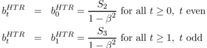
bHT Rt = bHT R0 = S2
1−β2 for allt≥0, teven bHT Rt = bHT R1 = S3
1−β2 for allt≥1, todd
The only statement left to prove are the tax cuts in periodst= 0,1. For periodst= 0,1we have uc,0−vx,0+λ0(ucc,0c0+uc,0+vxx,0(c0+g)−vx,0)−ucc,0 λ0 bHT R2,−2 = 0
uc,1−vx,1+λ1(ucc,1c1+uc,1+vxx,1(c1+g)−vx,1)−ucc,1 λ1 bHT R2,−1 = 0
Notice that the difference with (37) for t >1 is the presence of the terms ucc,0 λ0 bHT R2,−2 and ucc,1 λ1 bHT R2,−1.These are clearly negative, implying that for the considered utility functions we have
τ2 > τ0 τ3 > τ1
The statement in the last line follows immediately from the last FOC written. ¥
These results could be easily extended to the case of uncertainty only in period t = 1 as in Section 2.3.1, to show that if an adverse shock to g occurs taxes are lowered for the next N −1 periods and there is a cycle of orderN.
5.3
Numerical solutions
To write the model recursively we observe that the Lagrangean can be rewritten as L=E0 ∞ X t=0 βt©u(ct) +v(xt) +λtSt+uc,t(λt−N −λt)bHT RN,t−N (39) +ν1,t ¡ MHT R−bHT RN,t ¢+ν2,t ³ bHT RN,t −MHT R´o
for λ−1 = ... = λ−N = 0.In a full recursive formulation we would once more have the curse of dimensionality with a state space made up of 2N + 1 states hλt−1, ..., λt−N, bHT RN,t−1, ..., bHT RN,t−N, gt
i
just as before. To overcome this we use the condensed PEA again. The FOC show that this problem is easier to solve as there are only two expectations to approximate, Et(uc,t+Nλt+N), and Et(uc,t+N). We choose Xtcore = (λt−N, bHT RN,t−N, gt) and keep the same tolerance level as in the the model with buy back. Table 6 summarizes the number of linear combinations needed to approximate our expectations. Relative to Section 3.3 the required state space is larger - in some cases two linear combinations of residuals are needed. Effectively this means a total of five state variables is enough. The condensed PEA still dramatically reduces the state space and makes computation of a non-linear solution feasible.
Figure 8 shows the impulse response functions for a 10 period bond under hold to redemption with the same calibration as in the previous sections. We compare the policy with the case of a
one and 10 period bond and buyback. Thefigure is for the case when the government initially has no debt, so it is comparable to Figure 1. We see from the impulse response functions for tax rates that varying the maturity of the bond does affect optimal policy, even for initial zero debt.
INSERT FIGURE 8
In the buyback case of Sections 2 and 3, when initial debt is zero, bN,−1 = 0, Figure 1 showed that the government does not promise a cut in taxes. Only when the government is in debtbN,−1 >0 (or has assets), as in Figures 2 or 4, we observed the promise to cut (increase) taxes in N −1 periods. Figure 8 however shows that even in the case of zero initial debt taxes showfluctuations. Taxes increase on impact, the response is decreasing forN −1 periods, then it jumps at the time of maturity to start going back down after that and so on. The positive but decreasing response for the first N −1 periods is standard in optimal taxation models with serially correlated shocks, it would also occur under complete markets: the highergt on impact indicates thatgtwill also be higher in the next periods, and this generates higher taxes for the next few periods for the utility function considered. The jump in the response function at lagN is a reflection of the fact that there are cycles of order N, as suggested by Result 2 and as can be seen directly from the martingale condition (32). Strictly speaking λ is not a risk-adjusted martingale but one can say that it is a risk-adjusted martingale of cycle N15. The inital high and decreasing response echoes N periods later, this is because a high gt bumps up λt so it is optimal to set higher λt+N and so on.Even if gt+N may be close to its mean, the effect of today’s shock on λt+N drives taxes back up atN lags and the cycle starts again.
The intuitive reason that there are cycles of orderN is the following. One could think of writing the budget constraints under incomplete markets in discounted form as
∞ X j=0 βjuc,t+j uc,t e St+j = N X i=1
bHT RN,t−ipN−i,t for all t (40)
These discounted constraints hold in all periods if and only if the period−tbudget constraints (30) hold. But as should be clear from the proof of Result 2 this is not a very relevant condition: even if (40) holds we would easily violate the debt limits (29), since solutions of this equation for bN given a sequence of surpluses usually generates an unstable solution for issued bonds.
We could instead write the budget constraints as follows: ∞ X j=0 βjNuc,t+N j uc,t e St+N j =bHT RN,t−N, for allt
These are also necessary and sufficient for (30) , with the advantage that they guarantee that if we use these conditions to solve for the bN’s given surpluses bonds do not go to infinity. These conditions show that what is relevant is the link between today’s issued bonds and the surpluses in
1 5
N,2N,3N, ...periods from now. If today we have a bad shock and we issueN period bonds, when these bonds mature N periods from now there will be a need for higher taxes and a higher deficit, sobN,t+N will increase hence there will be a need for higher taxes and higher deficits in2N periods and so on. Therefore it is reasonable that there is a cycle of periodN and that optimal policy has the shape displayed in Figure 8. The optimal response to an unexpected shock is to promise future taxes that in part accomodate the additional debt servicing in the periods when today’s debt will have to be repaid.
Result 2 suggests that taxes in the first N −1 periods should be lower if the government is in debt. This suggests that optimal policy will be to lower taxes during the first cycle of N periods relative to later cycles. An additional role of commitment is indeed to promise a cut in taxes during the first cycle relative to the cycles later down the line. This is why in Figure 9, which looks at the case of initial debt, the main difference with Figure 8 is that the second peak in taxes is lower than thefirst peak, while the opposite is true in Figure 8.