Claremont Colleges
Scholarship @ Claremont
CMC Senior Theses CMC Student Scholarship
2016
Using a Data Warehouse as Part of a General
Business Process Data Analysis System
Amit Maor
Claremont McKenna College
This Open Access Senior Thesis is brought to you by Scholarship@Claremont. It has been accepted for inclusion in this collection by an authorized administrator. For more information, please [email protected].
Recommended Citation
Maor, Amit, "Using a Data Warehouse as Part of a General Business Process Data Analysis System" (2016).CMC Senior Theses.Paper 1383.
Claremont McKenna College
Using a Data Warehouse as Part of a General Business Process Data Analysis System
submitted to
Professor Beth Trushkowsky
by Amit Maor
for Senior Thesis Spring 2016 April 25, 2016
Table of Contents
Abstract ... 4
Section 2: Background ... 7
2.1 Background: Project ... 7
2.2 Background: Data models and data storage ... 7
3.1 The Network Model ... 10
3.2 The Relational model ... 12
Section 4: Designing a DBMS for Analytics ... 17
4.1 Column store data warehousing ... 18
Section 5: Amazon Redshift ... 22
Section 6: 2015-16 Laserfiche Clinic Project ... 24
6.1 Problem statement ... 24
6.2 The Clinic project: Overview of Architecture... 25
6.3 Future use of Redshift ... 28
Section 7: Conclusion ... 31
Abstract
Data analytics queries often involve aggregating over massive amounts of data, in order to detect trends in the data, make predictions about future data, and make business decisions as a result. As such, it is important that a database management system
(DBMS) handling data analytics queries perform well when those queries involve
massive amounts of data. A data warehouse is a DBMS which is designed specifically to handle data analytics queries.
This thesis describes the data warehouse Amazon Redshift, and how it was used to design a data analysis system for Laserfiche. Laserfiche is a software company that provides each of their clients a system to store and process business process data. Through the 2015-16 Harvey Mudd College Clinic project, the Clinic team built a data analysis system that provides Laserfiche clients with near real-time reports containing analyses of their business process data. This thesis discusses the advantages of Redshift’s data model and physical storage layout, as well as Redshift’s features directly benefit of the data analysis system.
Section 1: Introduction
Laserfiche is a software company that provides each of their clients a system to store, process, and analyze business process data. A business process is a set of repeated, related tasks undertaken by a company in their regular operations. Business processes be internal, like hiring an employee, or related to a company’s business operations, such as invoice processing. Through the 2015-16 Harvey Mudd College Clinic project,
Laserfiche is seeking to create a data warehouse system that provides these clients with near real-time reports containing analyses of their business process data. Current Laserfiche systems allow clients to view aggregations of data based on specific fields from their data (e.g., all business processes completed by the same employee). Through the project, the Laserfiche Clinic team aims to improve the tools Laserfiche provides its clients by creating a system that would produce analysis reports for their data, which would in turn help them gain insights into their data and make more informed business decisions.
In the past half-century, both the demand for and the capability of data storage and analysis technology have grown remarkably. From the early 1960s to 2015, the processing power of computers doubled approximately every two years; this
phenomenon, originally predicted by Gordon E. Moore, is now known as Moore’s Law (mooreslaw.org). As processing power improved through the 1960s and 1970s, it became possible to store increasing amounts of data on computers. And, as the amount of data grew, users needed a way to store and manage their data more effectively. This led to the emergence of Database Management Systems (DBMSs). Over the course of the next few
decades, DBMSs have become ubiquitous, and a popular way to store and manage data on a large scale. And, with companies analyzing and storing massive amounts of data, the specific DBMS a company uses and the way they use it can greatly impact the success of a company. Special DBMSs, called data warehouses, are specifically optimized for data analysis, and are becoming more important as data analysis becomes a priority for companies.
Through the Clinic project, Laserfiche is seeking to use a data warehouse in order to help provide better data analytics services to its clients. One of Laserfiche’s products is their business process automation software, which helps clients design custom
applications for their own business processes, but lacks the tools to perform sophisticated analyses of the data gathered from these processes. The Clinic project uses a data
warehouse, Amazon Redshift, in order to store business process data as part of the data analysis system. In Section 2 of this thesis, background information on the Clinic project, as well as some important concepts in data modeling and data storage will be provided. Sections 3 and 4 review two important historical changes in the structure and prevalence of DBMSs which led to the creation of Redshift. Section 5 examines Redshift’s attributes which are most important to the Clinic project. Section 6 discusses the Laserfiche Clinic project, and Redshift’s role in the success of the project. Future plans for using Redshift in the project are also discussed. Specifically, these future plans describe how the Clinic team intends to utilize Redshift’s optimizations for data analysis in order to improve the data storage and data analysis components of the system. The future plans include the way Redshift would be used in a fully completed system, as conceptualized by the Clinic team.
Section 2: Background
2.1 Background: Project
The Clinic project uses a data warehouse, Amazon Redshift, in order to store business process data as part of the data analysis system. The system extracts Laserfiche client data stored on Laserfiche servers and stores it in Redshift, which is designed for fast data analytics. The data is then extracted from the data warehouse and processed in order to prepare it for data analysis. Finally, the data is analyzed with a series of scripts which are designed to provide useful data analysis for any business process.
Redshift is a crucial part of the analysis system, as it provides the project with the flexibility to efficiently store and integrate data, as well as to quickly extract data through data analysis queries. Redshift was chosen over several other data warehousing options primarily for its use of the relational data model, and its optimizations for data analysis and analytics workloads. These design components are described in depth in Sections 3 and 4.
2.2 Background: Data models and data storage
The goal of a database is to model and store data from real world applications, such as business processes. To that end, we need a set of constructs with which to relate objects (or entities) from those real world applications. The constructs influence
expressibility, and what questions can be asked of the data. As a result, data types, which are how databases differentiate between different entities, and relationships are important because of the questions they allow a user to ask. These relationships are therefore
important to data analysis; thus, it is important to understand the different types of relationships between data types.
In general, three important types of relationships exist: one-many, many-to-many, and one-to-one. To help illustrate the differences between these relationship types, let us imagine that a dataset contains information on a soccer league; data types in that dataset would include players, coaches, teams, stadiums, sponsors, and so on. A one-to-many relationship between data types A and B is one in which an instance of data type A can be related to many instances of B, but not vice versa. In our example, the team-player
relationship would be considered a one-to-many relationship. A many-to-many
relationship between data types A and B is one in which an instance of data type A can be related to many instances of B, and vice versa. In our example, the relationship between players and sponsors could be considered many-to-many; a player can be sponsored by many different sponsors, and a sponsor could sponsor many different players. Lastly, a one-to-one relationship is one in which an instance of data type A can be related to only one instance of B, and vice versa. In our example, the relationship between teams and stadiums can be considered a one-to-one relationship; teams can only have one home stadium, and a stadium can only be home to one team. These relationship types can also be directional. This allows for expressibility of parent-child relationships, which are most often represented by directional one-to-many relationships. The network and relational models, discussed in Sections 3 and 4, support all relationship types discussed.
In a database, relationships between different types of data are defined using a data model. A data model can also inform how that data is stored in a database. A data model determines how the data is structured, and defines how relationships between
different types of data are expressed logically. For this reason, it is important that a data model be precise, meaning that there must not be ambiguity in how data is organized by a data model. A data model must also be intuitive, such that users can understand how their data is being organized. An intuitive data model also encourages effective collaboration.
A user can then design how to fit their data within the data model using a schema. A schema is a concrete description of all the different types of data within a dataset, as well as the relationships between different types of data. In the soccer league example, the schema would describe the attributes for players, coaches, and teams that would be stored in the database, as well as the relationships between those different data types. In this example, the schema would specify that the teams contain a certain number of players, each of whom has a name, date of birth, height, and so on. Schemas describe the organization and details of a dataset; in so doing, they also inform the user as to how to access, query, and modify their data within the database.
Individual data items within a database are called records. Using the above soccer league example, each player, along with all of the player’s information, would constitute a single record in the database. If a new player joins the league, that player’s information, including their name, date of birth, height, etc., is sent to the database all together as a record, and then inserted into the database. Teams themselves would also be considered records; those records could contain their home stadium, year of founding, and other players. Thus, records can contain other records as part of their information, establishing relationships between those data types. This becomes important for later discussion of the schema used in the data analysis system created by the Clinic team.
Section 3: The Network and Relational Data Models
This section discusses the emergence of the relational data model for data storage, a paradigm shift in DBMS design that was important to the creation of Amazon Redshift. This section highlights the ways the relational model improved usability and intuitiveness of DBMSs. The network model, which preceded the relational model, organizes
relationships between data types using set and record types, while the relational model uses data tables along with primary and foreign keys. This thesis argues that the relational model is simpler, more intuitive, and more scalable. Redshift uses the relational data model, described in Section 3.2. An understanding of the relational data model is important in order to understand the schema decisions made by the Clinic team. These decisions are described in Section 6.2.
3.1 The Network Model
The DBMS came to the fore of computational technology in the early 1960s, using a data storage model known as the network model. The network model allowed for many-to-many relationships, which, in turn, allowed for more expressibility in
relationships between data types. One of the first DBMSs to use the network data model was Charles Bachman’s Integrated Data Store (IDS), released in 1964. IDS, and the underlying network data model, were highly influential at the time (Haigh,
amturing.acm.org). The network model was considered progressive because it supported multi-parent and multi-child data types; as such, it lent itself to the expression of
The network model relies mainly on two data structures: record types and set types. Record types are synonymous to data types, and the network model uses record types to describe the attributes that all records of a certain type will have. In the network model, every record has a unique name, a location in the database, and various attributes as specified in the record type. The second data structure, which gave the network model the flexibility for which it became known, is the set type. The set type is how the network model describes directional relationships between data types. Each set is defined by three key elements: an owner record type (exactly one), a set name, and member record types. The owner record type specifies the record type from which the directional relationship can be made. An owner record type can be an owner record type in multiple set
relationships, and can also be a member record type in other sets. The set name and its unique ID identify the set. Finally, the member record types define the different possible endpoints for a relationship from the owner record type. A member record type can be a member record type in multiple sets.
The network model is space-efficient and allows for fast access to data. A system using the model only needs to store the owner record type, set name, and member record types. Because of this, the network model required little space beyond the set definitions and the data itself. Consequently, DBMSs using the network model were considered more space efficient than other alternatives. The network model also had a number of optimizations, such as allowing for contiguous storage of information that would frequently be accessed together, to improve the speed of network model DBMSs. As such, the network model provided good solutions for both the speed and space efficiency needs of their users.
However, the network model did have its shortcomings. Primarily, the network model did not have physical data independence. Physical data independence requires that a change in the physical structure of the data, such as the location of that data in memory or its ordering relative to other data, have no impact on the schema describing that data or the applications that accessing it. If a change occurs on the physical level in a DBMS using the network model, an application accessing data in that DBMS would also have to be modified. This is because access to data in the network model typically involves use of pointers to the physical location where that data is stored. Additionally, queries involving multiple sets and large amounts of data, such as aggregations, would execute slowly in the network model, as this would require using pointers to access data in multiple sets and records in order to retrieve data. This would be slow because this data would not be stored contiguously in memory; therefore, every individual data point in an aggregation would likely have to be accessed individually. These weaknesses are addressed by the relational database model, and make the relational model better suited to handling complex data, as well as large amounts of data.
3.2 The Relational model
In 1970, Edgar F. Codd introduced the relational database model; this was a completely new paradigm for data storage. Over the following few decades the relational model challenged and then surpassed the network model as the prominent DBMS
structure. Amazon Redshift uses a relational model; thus, the model is important to the Clinic team’s schema design, as well as the data analysis queries executed by their system. The relational model, which provided greater usability than the network model,
helped simplify the DBMS system. The relational model was simple enough that an employee of a company needed only know how to operate a DBMS, without necessarily knowing much about the internal workings of the system. Because of the lack of physical data independence in the network model, a user of a network DBMS would likely have to be more familiar with physical information about their data. The relational model was based on sets of tuples, which can easily be organized as tables. Note that this is a different definition of “set” than the one used in the network model. Because the relational model can easily be organized as a collection of tables, it also lent itself to organization in larger schema relating multiple tables. As a result, data analysis queries, which often aggregate over multiple tables and attributes, were more intuitive in the relational model.
Codd’s model was driven by his belief that users of a database should not care about how their DBMS stores their data, as would likely be the case with the network model. This meant his model had to have physical data independence. In the abstract of his paper, Codd asserts that “future users of large data banks must be protected from having to know how the data is organized in the machine (the internal representation). ... Activities of users at terminals and most application programs should remain unaffected when the internal representation of data is changed” (377). The need for physical data independence becomes more important as databases grow in size and complexity. Codd explains that this is because “in many commercial, governmental, and scientific data banks, however, some of the relations are of quite high degree (a degree of 30 is not at all uncommon). Users should not normally be burdened with remembering the domain [column] ordering of any relation” (380). Codd was concerned that high-degree would
increase the knowledge required of a user to operate a DBMS. The network model
requires domain-ordering information when adding and removing attributes and sets from a database, which would become quite burdensome in the larger relations to which Codd alludes. Codd did not want users to deal with the ordering of their data; to him, it was important that “users deal, not with relations which are domain ordered, but with relationships, which are their domain-unordered counterparts. … Each user need not know more about any relationship than its name together with the names of its domains [columns]” (Codd 380). To achieve this goal, Codd suggested that sets and set
relationships be replaced with tables, with a fixed number of columns and arbitrarily many rows. The tables were the relations upon which the relational model was based. Like a record in the network model, a row represented a single instance of the type described by the table; similarly, columns in tables would replace attributes in records. Tables would help describe relationships between data types.
The structural data independence guaranteed by Codd’s model allows DBMS users to be more flexible to changes in the structure of their data. If, for example, a user wanted to add an additional field to a relation, that user would not have to be concerned with how this would affect the physical storage of the data, as they would need to do in the network model. Some additional work would then need to be done by the DBMS to store the additional column; crucially to Codd’s philosophy, however, the user would not need to know what changes are being made and how the additional column is being stored.
The model also lent itself to separating data into multiple tables, which can help a user organize their data logically. To make this possible, Codd had to devise a way to
separate data into multiple related tables; for this, Codd introduced the idea of primary and foreign keys (380). Codd defined a primary key as one or more columns in a table that uniquely identified each row, and a foreign key as one or more columns in a table that reference a column (possibly the primary key) in a different table. These features encouraged users to devise schema consisting of multiple tables, each containing subsets of the data.
The Clinic team’s schema for storing business process data is called a star schema. A star schema involves a central table, called a fact table, where each row represents a single record for a particular business process. This table has few columns, most of which are foreign keys to other tables, known as dimension tables. These
dimension tables contain information relating to the business processes in the central fact table. This overall schema is flexible, because the dimension tables can collectively store all data types for any business process. This is important to the Clinic team because the schema is intended to work for any business process. The schema is described in further detail in Section 6.2.
From Codd’s work, a new form of DBMS, the relational DBMS (RDBMS), was born. Requiring a user to keep track of the ordering details of their data can be
impractical; this is especially true in relations containing dozens of columns, as can be the case with business process data. Thus, because of the physical data independence of the relational model, the RDBMS required less user expertise than the network DBMS did. For the Clinic project, this is important because the project aims to reduce the amount of work and DBMS expertise required of Laserfiche clients to store and analyze data. The RDBMS also made data analysis more intuitive; with data separated into
multiple tables in a known schema, a data analysis query can be as simple as aggregating over the desired columns in various tables. This is important to the Clinic project because the analysis system aggregates over multiple tables in the schema for business process analysis.
Section 4: Designing a DBMS for Analytics
The second major change in the DBMS landscape is that of data warehouses, which are DBMSs designed specifically for analytics. To understand how a DBMS can be designed for this purpose, we need to differentiate between the two main types of database workload: transactional and analytical. In conjunction with these two workload types are the two main types of database processing, which are on-line transactional processing (OLTP) and on-line analytical processing (OLAP). The two workloads differ in the types of queries most frequently executed; this makes it possible to design a DBMS to be optimized for one of these workloads. Amazon Redshift, for example, is optimized for OLAP workloads. This is discussed in greater detail in this section, as well as in Section 5.
OLTP databases work best in environments where the user needs to perform many smaller individual transactions using the database, such as updates, inserts, and deletions. OLTP databases often contain high volume writes (as opposed to reads), as would be the case in a company’s operational database. This is where a company would keep track of banking transactions, enter online shopping orders or updates, or similar tasks. Generally speaking, “these tasks are structured and repetitive, and consist of short, atomic, isolated transactions” (Chaudhuri 517). As such, fast query processing and accuracy are the most important indicators of a successful DBMS designed for OLTP workloads; these types of actions are often measured in transactions per second or a similar metric. Because of the high volume of transactions in such a database, “the database is designed … in particular, to minimize concurrency conflicts” (Chaudhuri
517). Though all databases ensure data is not lost if multiple queries or transactions are executed concurrently, Chaudhuri explains that DBMS optimized for OLTP workloads will be designed specifically to handle concurrency conflicts and minimize their effects.
Because OLTP databases are primarily optimized for high-volume writes, companies often prefer to separate their read-heavy workloads into a different database which is optimized for reads over large amounts of data. DBMSs designed for OLAP workloads, known as data warehouses, are optimized for lower volume of writes and higher volume reads and aggregations of existing data. OLTP databases typically contain less data than data warehouses, and generally do not contain all data from a business process; this is because it is unlikely that a company will need to access old business process data, known as historical data, for their day-to day transactions. Because data warehouses often store massive amounts of historical data, fast performance for large queries and aggregations is most important for a successfully designed data warehouse. Amazon Redshift’s performance in these areas was an important factor when choosing to use it in the analysis system built for the Clinic project.
4.1 Column store data warehousing
There are a number of database design improvements that can be made (by a company such as Amazon) in an RDBMS in order to optimize for OLAP workloads. Optimizing for analytics can be challenging; this is because “while CPU performance and available cache memory has increased dramatically with 64-bit servers and lower
memory prices, disk performance has not kept up and, consequently, disk-bound performance is typical for many analytics” (MacNicol, 1227). As such, it is important
that an RDBMS minimizes the number of disk reads made by the system. To do so, the information that is most often read together by users needs to be stored contiguously. This is especially important for analytics workloads. Since analytics queries often access much more data than transactional queries, they are more likely to require multiple disk reads; because disk reads are by far the most time-costly component of an analytical query, they have the potential to drastically decrease performance.
Concerns over disk reads, and performance in queries accessing massive amounts of data, motivated the use of column-stores, as opposed to row-stores, for data
warehousing. In the 1990s, Sybase spearheaded the use of column-stores for data analysis. The use of column-stores represented a radical change in internal database design. And, because the demand for big data analytics continued to grow through the following decades, the design change was crucial in helping solve what Sybase call the “data explosion problem” (MacNicol 1227). In traditional transaction workloads, it makes sense to store the data of an entire record contiguously, as it would optimize for inserting, deleting, and updating data instances. However, this design would not work well for OLAP workloads. Sybase noted that “typical analytical queries access relatively few columns of the storage-dominating fact tables and may access a notable proportion of the rows stored in the fact tables” (MacNicol 1227). Because analytics queries access few columns and large numbers of rows, it made more sense to store the information with column data stored contiguously, rather than row data. And, while this would increase the time taken to perform transactions such as inserting new records, this was a tradeoff that would make sense for analytics; “since data is only written once but read many times any increase in load time would be more than offset by improved query performance”
(MacNicol 1228). This is further reinforced by Stonebraker, who asserts that “in
warehouse environments where typical queries involve aggregates performed over large numbers of data items, a column store has a sizeable performance advantage”
(Stonebraker 1).
Sybase also made additional design changes; they decided to have larger page sizes to minimize physical disk reads, which are by far the slowest part of responding to a query, and index columns instead of rows for quicker access to columns for querying. These design changes were also adopted by Amazon in their design of Amazon Redshift. The indexing optimization is especially important because a user may want to add or delete columns based on changing business needs of a company. With the new design, “Adding or dropping a column or index to reflect changing business requirements would be cheap, as no other data would be accessed” (MacNicol 1228). Thus, the design changes introduced by Sybase, especially the introduction of the column-store, lend themselves much more effectively to the handling of OLAP workloads than had row-store RDBMSs.
An example involving a transactional query and an analytics query makes it easy to see why this is the case. In our soccer example, let us imagine that a user wants to add another player to the warehouse. This would be faster in a row-store, as all the player’s information (that is, the row) would be stored contiguously on the disk. In a column store, where data for each attribute, rather than each player, would be stored contiguously on the disk, all player names would be stored next to each other, all player heights would be stored next to each other, and so on. Thus, the column-store RDBMS would have to jump
from attribute to attribute to insert the new data, which could increase the number of disk reads and take longer as a result.
Now, let us imagine that the user wants to know the average height across all players in the data warehouse. In a row-store, the RDBMS would have to jump from player to player to extract each player’s height, which would likely access a large amount of disk space and likely require multiple disk reads. On the contrary, if a column-store database were to handle a query for the average height, the RDBMS would simply access the index of the column containing height data and grab all the heights from the various students. As such, the column store would require substantially fewer disk reads, and potentially just a single read, if the number of players does not exceed the page size. This example helps illustrate the magnitude of the performance boost that a column-store can provide for data warehousing and OLAP workloads. The query in this example is similar to many of the queries the Clinic project’s data analysis system executes in Redshift, which involve a small number of columns and a large number of rows.
Section 5: Amazon Redshift
Amazon Redshift is the data warehouse offered by Amazon as part of their Amazon Web Services (AWS) platform. This section describes Amazon Redshift, and focuses more specifically on the features of Redshift which are most important to the Clinic project.
Redshift is capable of storing petabytes of data, which, as discussed above, is important for a data warehouse, which often holds massive amounts of historical data. All user data is stored on Amazon servers that are maintained and operated by Amazon. Redshift also manages the user’s data and databases. This means that Redshift
automatically backs up the user’s data on other Amazon servers and provides additional processing power to the user’s databases as needed. Processing power is increased by adding compute nodes, which are the basic unit of server space on which a user’s queries can be run. In the context of the Clinic project, these are maintenance tasks that the Laserfiche client would not have to worry about; their data would be backed up automatically, and they would never have to worry if the warehouse has enough processing power to handle their workload.
Amazon Redshift uses a relational model to store data. As discussed above, the relational model reduces the amount of information a Redshift user needs to know about the way their data is stored. The user does not need to know the order of the columns in tables or other minutiae that can greatly increase the knowledge required of the user. Redshift is also cloud-based, meaning that users access the data warehouse using the Internet, and do not need to know where their data is stored. This also makes it easier for
Redshift to be offered as part of a separate Web application, as would be the case with the data analysis system created for Laserfiche. The interested reader can learn more about cloud computing in “A view of cloud computing” (Armbrust et. al.)
Redshift has additional features to increase its speed of its data analysis queries, which made it well suited to the needs of the 2015-16 Laserfiche Clinic project. The most important feature for the purposes of the Clinic project is the use of massive parallel processing (MPP). Amazon describes MPP as “parallelizing and distributing SQL
operations to take advantage of all available resources” (Amazon Redshift page), dividing work between its huge number of servers in order to execute queries and aggregations as fast as possible. This is important because it improves performance for queries that access massive amounts of data. The Laserfiche Clinic data analysis system currently handles about 20,000 rows of internal Laserfiche business process data; as such, it does not make much use of Redshift’s MPP architecture. However, the MPP architecture will become more important as the analysis system handles more business process data from multiple Laserfiche Clients. This is further discussed in Section 6.
Section 6: 2015-16 Laserfiche Clinic Project
The purpose of this section is to motivate the importance of the Clinic project, and the importance of Redshift to the success of the project. After introducing Laserfiche and the problem they presented the Clinic team, an overview of the architecture of the data analysis system created by the Clinic team will be discussed. In particular, the section will focus on the design decisions that prepare the data analysis system to take advantage of Redshift’s strengths in the future. Then, attention will be turned to exactly how the Clinic team intends to take advantage of Redshift once the system is being used by Laserfiche and its clients.
6.1 Problem statement
As discussed in the introduction to this thesis, Laserfiche is seeking to create a data analysis system that provides their clients near real-time analysis reports for their business process data. The company currently offers business process automation software, which allows clients to design custom applications to keep track of their own business processes. Still, their software does not allow for the sort of large scale data analysis that works best using a data warehouse like Amazon Redshift. As such,
Laserfiche have asked the Clinic team to create an analysis system that their clients can use to analyze their business process data. As part of this system, Laserfiche ask that a data warehouse be used, and that data for all their clients is stored in that data warehouse.
The job of the data analysis system is to analyze Laserfiche clients’ business process data. Additionally, Laserfiche wants the system to be general, meaning that it will
produce useful analysis results regardless of the business process contained in a dataset. Thus, the system needs to successfully store and analyze data without knowing what business process is being stored and analyzed. This meant that schema used in Redshift would also have to be as general and flexible as possible, in order to handle data from any business process. This led to our design of a generalizable schema, which can organize data for storage in Redshift for any business process.
6.2 The Clinic project: Overview of Architecture
The system relies on Amazon enterprise products for data migration and storage. To transfer data from Laserfiche’s business process management (BPM) servers, where Laserfiche clients’ business process data is currently stored, to Amazon Redshift, we use Amazon Kinesis. This step is called the “data migration step,” because we migrate the data from Laserfiche servers to Redshift. Kinesis’s main functionality is as “a platform for streaming data” (Amazon Kinesis page), meaning that Kinesis receives data from a source (in our case, a Laserfiche BPM server) and “streams” the data to another location (in our case, Amazon Redshift). Once data is sent from the Laserfiche BPM servers to Kinesis, it is held in Kinesis until it is fetched by a program that inserts it into Redshift. Amazon Kinesis provides different channels, called streams, by which to group data separately, and which will eventually be used in order to separate the data of different companies' business processes. The analysis system is built to store data from each individual Laserfiche client in a separate database, and each database will have several tables organized together in a multidimensional schema.
We had to devise a storage schema that would store business process data for all of Laserfiche’s customers, and also to make use of Redshift’s optimizations for data analysis. To achieve these goals, we devised a general star schema for business processes. Recall that a star schema is a multidimensional schema consisting of a central fact table surrounded by multiple dimension tables. The fact table contains information about every individual business process record, with foreign keys in the fact table linking to the dimension tables. The fact table also contains measures, which are important quantitative data about business processes, such as the price of a transaction. Dimensions hold
important auxiliary information about business processes, such as the time of the
transaction or the employee who was involved in the transaction. The foreign keys in the fact table are also primary keys in the dimension tables, such that each entry in the dimension tables (as well as the fact table) is uniquely identifiable. Our star schema is designed to work for any business process.
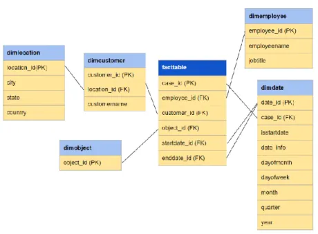
Our schema, shown below in Figure 1, captures the logical structure common to all business processes. The central fact table contains the unique primary key ID attached to every business process record, foreign keys to four dimension tables, and context-specific measures that are not shown in the general diagram. The four dimensions are the employee, customer, date, and object dimensions. We believed these dimensions would be consistent across all business processes. The employee dimension describes
employees from the company using the Laserfiche software; the customer dimension describes a potential third party, such as a customer in a sale or a potential new employee in a hiring process who is not affiliated with the company using the software; the date dimension provides timestamps and additional time information for business process
instances; and the object dimension table is a table designed to accommodate important context-specific details, such as “product category” for a sales business process or “operating system” for a tech support business process.
Figure 1: The generalized star schema for storing business process data in Redshift.
With these four main dimension tables, measures, and a location dimension table to provide optional additional information about customers, we feel that the schema can organize data from all business processes.
Once the data is stored in Redshift according to the schema, the system can query the database in order to aggregate information and extract it for analysis. Once the data in analyzed, the results are output to another file. The eventual goal is to display the results to the user on a dashboard.
These schema and system decisions were made with the intention of utilizing Redshift’s strengths in the future, most importantly scalability and performance on queries involving massive amounts of data. The star schema will organize data from any business process. The program that fetches data from Kinesis and inserts it into Redshift also simplifies the process of adding columns in Redshift. To add columns, a Laserfiche client simply stores new data on the BPM server containing the new column; the data is then sent to Redshift through Kinesis, and if the columns in the new data do not match the columns in the schema, the program inserting records into Redshift will add or delete columns in the database as necessary. This process has good performance in Redshift, as the column-store design and column indexing ensure this process is as simple as
removing a contiguous block of data, representing a single column. Most importantly, the system will also eventually take advantage of optimizations for data analysis that are offered through Amazon Redshift. This is described further in Section 6.3.
6.3 Future use of Redshift
As mentioned in Section 5, our current use of Redshift is in our proof-of-concept prototype, holding about 20,000 rows of data relating to an internal Laserfiche business process. As such, none of Redshift’s optimizations for massive amounts of data are currently being exercised by the system. However, as the amount of data in the system grows, and speed and scalability become important, Redshift’s strengths in storing
massive amounts of data and performing fast data analysis queries will contribute directly to the success of the analysis system. To help illustrate this, let us imagine that the system
is being used by hundreds of Laserfiche customers for thousands of business processes, as the system is designed to eventually do.
Because Redshift is fully managed by Amazon, the resources devoted to Laserfiche’s clients in Redshift will grow as the analysis system’s workload grows. In fact, if either the workload or the amount of data becomes sufficiently large, Amazon will provide more processing power to the cluster as necessary, and even reorganize the hardware space devoted to Laserfiche data to be as efficient as possible. Importantly, even as the quantity of data in the system grows, the schema design will never need to change.
Just as importantly, as the magnitude and quantity of client queries grow, Amazon Redshift should still be able to handle the queries quickly, due to Redshift’s many
optimizations for data analysis queries. Even though the actual analysis of data occurs outside of Amazon Redshift, the data warehouse can increase the performance of the analysis scripts by ensuring that the process of extracting data from Redshift occurs as efficiently as possible. To this end, future work on the analysis system could include temporarily storing the results of queries such that they do not have to be called multiple times. An object that stores the results of a query is called a materialized view; if the same data needs to be fetched from Redshift for several different queries, a materialized view could improve the performance of those queries by providing faster access to the necessary data. This optimization can further improve the system’s efficiency in
retrieving information for data analysis, as queries to a materialized view would be more efficient than queries to the entire database.
Other Redshift optimizations will also prove useful once the system is used at full capacity. By splitting large, simple aggregations and queries and executing them in parallel across multiple nodes, Redshift’s MPP architecture will make sure that
aggregations are being run as fast as possible. The cloud-based component will also be helpful to Laserfiche’s many clients around the world. This is especially true for
Laserfiche clients with employees in multiple locations, who will not need to worry about their proximity to their data warehouse or to each other. These design decisions, which were made to optimize for OLAP workloads, will ensure that even when the system manages large quantities of data, the performance of the system will be sufficient for the needs of Laserfiche users.
Section 7: Conclusion
The “data explosion problem,” and the general trend towards more big data in the technology industry, have dramatically increased the need for high performance
RDBMSs optimized for OLAP workloads. The historical foundations for these changes can be traced back to the shift from the network model to the relational model. This change was crucial in providing RDBMSs with scalability and flexibility, as it provided physical data independence and ease of use, which in turn allowed for decreased
specialization from users and increased accessibility to data analysis.
In response to the demand for data analytics that precipitated these technological innovations, Laserfiche has asked the 2015-16 Clinic team to use a data warehouse as part of a generalizable data analysis system. The product chosen for the data warehouse component was Amazon Redshift. Redshift would be responsible for two distinct tasks. The first task is storing massive amounts of business process data and organizing it logically in a star schema. The second task is to respond quickly to data analysis queries. The latter task is the primary reason for which Redshift was chosen.
The Clinic team’s analysis system will hopefully provide Laserfiche clients with timely insights and analysis, all while requiring little active involvement from the clients. The schema in Redshift is designed to store and organize data for any business process, such that the client will not have to fine-tune the system for their specific business process data. And, importantly, queries to the data warehouse for analysis will be fast, due to the many optimizations provided by Redshift for OLAP workloads. As part of the 2015-16 Laserfiche Clinic team’s data analysis system, Amazon Redshift should help
Laserfiche clients understand their business processes, make informed changes and decisions, and ultimately succeed in their businesses.
Bibliography
"Amazon Kinesis – Amazon Web Services (AWS)." Amazon Web Services, Inc. N.p., n.d. Web. Apr. 2016.
"Amazon Redshift – Data Warehouse Solution – AWS." Amazon Web Services, Inc. N.p., n.d. Web. Apr. 2016.
Armbrust, Michael, et al. "A view of cloud computing." Communications of the ACM 53.4 (2010): 50-58.
"Big Data Solutions – Amazon Web Services (AWS)." Amazon Web Services, Inc. N.p., n.d. Web. Apr. 2016.
Chaudhuri, Surajit, and Umeshwar Dayal. "An overview of data warehousing and OLAP technology." ACM Sigmod record 26.1 (1997): 65-74.
Haigh, Tom. "Charles W. Bachman - A.M. Turing Award Winner." Charles W. Bachman - A.M. Turing Award Winner. N.p., n.d. Web. 18 Apr. 2016.
MacNicol, Roger, and Blaine French. "Sybase IQ multiplex-designed for
analytics." Proceedings of the Thirtieth international conference on Very large
data bases-Volume 30. VLDB Endowment, 2004.
"Moore's Law." Moores Law. N.p., n.d. Web. 18 Apr. 2016. <http://www.mooreslaw.org/>.
Stonebraker, Mike, et al. "C-store: a column-oriented DBMS." Proceedings of the 31st international conference on Very large data bases. VLDB Endowment, 2005. Taylor, Robert W., and Randall L. Frank. "CODASYL data-base management