Generated using version 3.0 of the official AMS LATEX template
Weak pressure gradient approximation and
its analytical solutions
David M. Romps
∗Dept. of Earth and Planetary Science, University of California, Berkeley
Earth Sciences Division, Lawrence Berkeley National Laboratory
Berkeley, California, USA
∗Corresponding author address: David M. Romps, Department of Earth and Planetary Science, 377
ABSTRACT
A weak-pressure-gradient (WPG) approximation is introduced for parameterizing supra-domain-scale (SDS) dynamics, and this method is compared to the relaxed form of the weak-temperature-gradient (WTG) approximation in the context of 3D, linearized, damped, Boussinesq equations. It is found that neither method is able to capture the two different timescales present in the full 3D equations. Nevertheless, WPG is argued to have several advantages over WTG. First, WPG correctly predicts the magnitude of the steady-state buoyancy anomalies generated by an applied heating, but WTG underestimates these buoy-ancy anomalies. It is conjectured that this underestimation may short-circuit the natural feedbacks between convective mass fluxes and local temperature anomalies. Second, WPG correctly predicts the adiabatic lifting of air below an initial buoyancy perturbation; WTG is unable to capture this nonlocal effect. It is hypothesized that this may be relevant to moist convection, where adiabatic lifting can reduce convective inhibition. Third, WPG agrees with the full 3D equations on the counterintuitive fact that an isolated heating applied to a column of Boussinesq fluid leads to a steady ascent with zero column-integrated buoyancy. This falsifies the premise of the relaxed form of WTG, which assumes that vertical velocity is proportional to buoyancy.
1. Introduction
A wide range of scales contribute to the dynamics of the atmosphere, from cloud eddies at tens of meters to planetary scale circulations at tens of thousands of kilometers. It is impossible to capture all of these scales in a single numerical simulation, so some range of scales must be parameterized. The approach taken in general circulation models (GCM) is to resolve large-scale circulations and parameterize small-scale convection. The approach taken in cloud-resolving models (CRM) is to resolve small-scale convection and parameterize large-scale circulations. The former is often referred to as sub-grid-large-scale (SGS) parameterization; we can refer to the latter as supra-domain-scale (SDS) parameterization.
In a CRM, the simplest way to parameterize the large scale is to impose a profile of ascent or subsidence. The downside of this approach is that it decouples the large-scale vertical velocity from convection. An alternative is to parameterize the vertical velocity using the weak-temperature-gradient (WTG, Sobel and Bretherton 2000) approximation. In the most common implementation of WTG, the vertical advection of virtual potential temperature, (w∂zθv), is assumed to remove differences in buoyancy (∆θv) between the CRM and the
larger environment over a fixed timescale (τ) (e.g., Raymond and Zeng 2005; Raymond 2007; Sessions et al. 2010; Wang and Sobel 2011, 2012). Therefore, the vertical velocity in this relaxed form of WTG is specified as w = ∆θv/(τ ∂zθv). In practice, this formulation
performs poorly at altitudes where the static stability approaches zero, such as in the dry boundary layer. The remedy commonly used for the boundary layer is to linearly interpolate w from its predicted value above the boundary layer to zero at the surface (e.g., Sobel and Bretherton 2000; Raymond and Zeng 2005). The scheme also produces w values that are often too large in the upper troposphere (e.g., Raymond and Zeng 2005). This is combatted by replacing∂zθv with max(γ, ∂zθv) for some constantγ >0, and by modulating the resulting
velocity by a factor that tapers to zero in the upper troposphere (e.g., Raymond and Zeng 2005; Sessions et al. 2010).
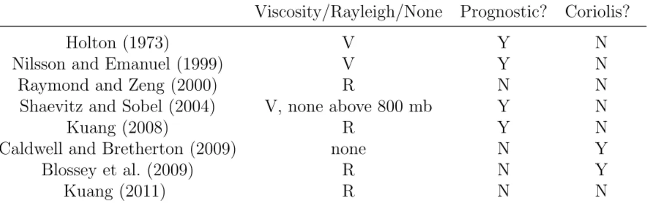
The ad hoc nature of these required fixes suggests that WTG may not be capturing the relevant dynamics. This is also suggested by the fact that the basic premise of the relaxed form of WTG – that the vertical velocity is proportional to buoyancy with a fixed timescale – is not derived from the governing equations. An alternative approach, which we refer to here as the weak-pressure-gradient (WPG) approximation, is to derive an expression for the vertical velocity directly from the momentum equations (e.g., Holton 1973; Nilsson and Emanuel 1999; Raymond and Zeng 2000; Shaevitz and Sobel 2004; Kuang 2008; Caldwell and Bretherton 2009; Blossey et al. 2009; Kuang 2011). Although these studies differ in the details of their implementation of WPG (see Table 1), their common feature is a parameterization of the pressure-gradient force between the column and its environment. The direct effect of this parameterized momentum equation is to produce weak gradients of pressure.
The goal of this paper is to compare the accuracy of WTG and WPG using analytical solutions to linearized Boussinesq equations. Section 2 reviews the relevant three-dimensional Boussinesq equations and presents two analytical solutions to these 3D equations: a transient solution in which a buoyancy anomaly is carried out of a column by gravity waves, and a steady solution in which a heating applied to a column leads to steady-state profiles of buoyancy and vertical motion. The two different timescales inherent to these solutions will be of particular interest. Section 3 introduces the WTG approximation and derives the transient and steady-state solutions analogous to the full 3D solutions. Section 4 introduces the prognostic WPG approximation and also derives the analogous transient and steady-state solutions. Section 5 introduces the diagnostic WPG approximation and its solutions. These four sets of transient and steady solutions – i.e., in 3D, WTG, prognostic WPG, and diagnostic WPG – are compared to one another in section 6. This illuminates some deficiencies of the WTG method that are remedied by the WPG method. A brief summary is given in section 7. Finally, the appendix describes a formulation of WPG for cloud-resolving models, which is used by Romps (2012) to follow up on the analytical results presented here.
2. Full 3D equations
The linear, hydrostatic, Boussinesq equations in 3D with Rayleigh drag are ∂tu = − 1 ρ∂xp−αu (1a) ∂tv = − 1 ρ∂yp−αv (1b) 0 = B− 1 ρ∂zp (1c) ∂tB = −N2w+Q (1d) ∂xu+∂yv+∂zw = 0. (1e)
Here, a hydrostatic background state has been subtracted, so pis the pressure perturbation (Pa) andB is the buoyancy (m s−2). The other variables take their usual meaning: α is the Rayleigh drag coefficient (s−1), ρ is the constant density (kg m−3), N is the Brunt-V¨ais¨al¨a
frequency (s−1),Qis the applied buoyancy source or heating (m s−3), andu,v, andware the velocities (m s−1) in the x, y, and z directions, respectively. The symbol ∂t is a shorthand
for the partial derivative with respect to time, and similarly for subscriptsx,y, andz. These equations can be combined into a single equation for B,
∂t2∂z2B +α∂t∂z2B+N
2∇2B = ∂
t∂z2Q+α∂
2
zQ . (2)
Here, ∇~ is the two-dimensional gradient operator.
We will focus on two prototypical solutions. The first is an adiabatic (Q = 0) transient solution in which we use α = 0 for simplicity; setting α to zero in these solutions is a reasonable approximation so long as 1/α is large compared to the timescale λ discussed below. This transient solution will represent a buoyancy perturbation initially confined to a motionless column of horizontal scaleL. Of particular interest will be the transient timescale λthat describes how long it takes the buoyancy perturbation to propagate out of the column. We can investigate this by studying the time dependence of the solution at the center of the column (i.e., at r = 0), or by studying the average evolution of the solution within some finite radius (i.e., r < L).
The second prototypical solution is a steady state in which we use α > 0 and apply a steady heating (Q6= 0) in a column of horizontal scaleL. In this case, we will be particularly interested in the steady timescaleσthat relates the magnitude of the buoyancy perturbations to the heating Q. Again, since we are interested in the behavior of the column, we will want to study the solution at r = 0. For both solutions, we will assume a rigid free-slip bottom and top at z = 0 andz =H, respectively. The free-slip condition is appropriate for a model of the free troposphere, and the rigid boundaries (to be thought of as representing the top of the boundary layer and the tropopause) are a mathematical convenience.
Let us begin with the transient solution. When α and Q are both zero, equation (2) simplifies to ∂2
t∂z2B +N2∇2B = 0. This equation reveals that a buoyancy perturbation
of vertical wavenumber m and horizontal scale L has a characteristic timescale of mL/N. We seek a solution to this equation that is cylindrically symmetric and has a buoyancy perturbation centered at the origin with a horizontal scaleLand amplitudeB0. The simplest
such solution is B = B0 2π Z 2π 0 dφ exp " − rsinφ−N mt 2 /L2 # sin(mz), (3)
where r = px2+y2. This solution is shown at two different times in the top panels of
Figure 1. At r = 0, this buoyancy evolves as B|r=0 = B0exp h −(t/λ3D)2 i sin(mz). (4) where λ3D = mL N . (5)
This is the timescale over which the column’s buoyancy perturbation decays to zero in the 3D transient case.
Next, let us construct the steady-state solution. When α and Q are nonzero and there is no time dependence, equation (2) reduces to ∇2B = α
N2∂z2Q. This equation reveals that
(m s−2) that is related to the magnitude of the heating (m s−3) by the timescale αλ2 3D. We
seek a solution to this differential equation in which Q and B are cylindrically symmetric and centered on the origin with a width of L. The simplest such solution is
Q = Q0 1− r 2 4L2 exp − r 2 4L2 sin(mz) B = αm 2L2 N2 Q0exp − r 2 4L2 sin(mz), where Q0 is a constant. At r= 0, this solution can be written as
Q|r=0 = Q0sin(mz) (6)
B|r=0 = σ3D Q|r=0 . (7)
We see, as expected, that B (m s−2) andQ (m s−3) are related by a timescale of
σ3D = αλ23D. (8)
This is the timescale that relates the magnitude of the column’s buoyancy perturbations to the magnitude of the applied heating.
These three-dimensional solutions provide a benchmark against which the WTG and WPG approximations can be evaluated. Since WTG and WPG are designed to parameterize the dynamical interaction between a disturbed column of fluid and its quiescent environment, they should be able to reproduce the behavior of these solutions at r= 0. In particular, we have derived two different timescales – λ3D for transients and σ3D for steady states – that
WTG and WPG should be able to replicate.
3. WTG approximation
The weak-temperature-gradient (WTG) approximation reduces the full 3D equations to a set of 1D equations in which the dynamical interaction between the column and its envi-ronment is parameterized. WTG accomplishes this by parameterizing the vertical advection term in the thermodynamic equation. In this paper, we focus on the relaxed form of WTG introduced by Raymond and Zeng (2005). The assumption therein is that vertical motion consumes buoyancy perturbations with some constant timescale τ, i.e., wN2 =B/τ; in the
limit of τ = 0, this reduces to the strict WTG introduced by Sobel and Bretherton (2000). In the Boussinesq system, these WTG equations are described by
0 = B − 1
ρ∂zp (9a)
∂tB = −N2w+Q (9b)
w = B
τ N2 . (9c)
The differential equation for B becomes
∂tB = −
B
where τ is a constant that must be chosen a priori. Note that this equation is qualitatively different from equation (2), which was derived from the three-dimensional equations.
In the full 3D system, equation (2) contains two constants, 1/αand 1/N, which allow its solutions to exhibit two distinct timescales, λ3D and σ3D. In WTG, equation (10) contains
only one constant,τ. This means that it is not possible to simultaneously represent transient and steady-state behavior faithfully with WTG unless, by coincidence, the two timescales λ3D and σ3D are the same. Instead, the value of τ must be chosen based on whether the
accuracy of transients or steady states is more important.
WTG admits solutions that are analogous to the solutions in the previous section. By choosing
τ = πL
N H , (11)
a transient solution in the absence of heating isB =B0exp(−t/λWTG) sin(mz), which decays
to zero with a timescale of
λWTG = τ =
π
mHλ3D. (12)
This matches the 3D transient timescale λ3D if m = π/H. In other words, this gives the
correct transient timescale for the first baroclinic mode. For higher baroclinic modes (i.e., m > π/H), transient perturbations are overdamped: they decay with a timescale that is too short by a factor of π/mH.
Equation (11) is not the correct choice for steady-state solutions. Instead, we must choose τ = π
2αL2
N2H2 , (13)
in which case the steady-state solution to Q =Q0sin(mz) is B =σWTGQ with a timescale
of σWTG = τ = σ3D π mH 2 . (14)
This matches the 3D steady timescale σ3D if m=π/H. For m > π/H, the WTG timescale
will be too small by a factor of (π/mH)2. This implies that the magnitude of the buoyancy
will be too small by this factor.
4. WPG approximation, prognostic
In the weak-pressure-gradient (WPG) approximation, we reduce the full 3D equations to a set of 1D equations by parameterizing the horizontal Laplacian of the pressure. Be-ginning with the full 3D equations (1a–1e), we add ∂x of (1a) and ∂y of (1b) to get ∂tδ =
−(1/ρ)∇2p−α∗δ, where δ≡∂
xu+∂yv is the horizontal divergence. Here, we have denoted
the damping rate by α∗ since it is a free parameter that we may or may not want to set equal to the Rayleigh damping rate α. We now assume that the column being modeled has a constant horizontal scale L and is embedded in an environment with zero perturbation
pressure, in which case we can approximate ∇2p as−p/L2. This gives the WPG equations, ∂tδ = 1 ρ p L2 −α ∗ δ (15a) 0 = B− 1 ρ∂zp (15b) ∂tB = −N2w+Q (15c) δ+∂zw = 0. (15d)
These can be reduced to a single equation in B, ∂t2∂z2B +α∗∂t∂z2B− N2 L2B = ∂t∂ 2 zQ+α ∗ ∂z2Q . (16)
Note the similarity between equations (16) and (2).
When Q=α∗ = 0, the differential equation becomes ∂t2∂z2B− N2
L2B = 0. We might hope
that this equation would have (4) as a solution, but it does not. Instead, the solutions to this equation are of the form exp(iωt−imz) with ω = ±N/mL. In other words, the solutions correspond to a column immersed in an infinite bath of plane waves, which is not what we want.
We will now solve for the transient solution while keeping α∗ nonzero. When Q= 0, the plane wave exp(iωt−imz) is a solution to (16) so long as ω satisfies a dispersion relation,
ω = i(α∗/2)±p−(α∗/2)2+N2/(m2L2).
If we set α∗ equal to the true Rayleigh damping rate α, and if α N/mL (i.e., if gravity waves propagate out of the column much faster than they are damped), then the solution still oscillates with a timescale of aboutmL/N. The solution is damped, but on a timescale of 2/α, which is much longer than λ3D =mL/N.
In order to generate damping on a timescale comparable tomL/N, we can co-optα∗ to represent the timescale with which waves propagate out of the column. Of course, we only have the latitude to pick a single value for the constantα∗, so we must pick anα∗ that gives the correct timescale for the mode of most interest. For our purposes, we will pick
α∗ = 2HN
πL (17)
so that the first baroclinic mode (which hasm=π/H) will decay with the correct timescale. With this choice for α∗, modes of general m will decay as a sum of two exponentials with timescales λ± = λ3DF±(mH/π), where F±(x) = 1 x 1± s 1− 1 x 2 −1 .
This function gives the ratio of λ+ and λ− to the correct timescale for vertical wavenumber m. Note that F±(1) = 1. For integerx > 1, a good approximation to F±(x) is (2x)∓1. In other words,
F±(x) ≈
(
1 x= 1
(2x)∓1 x >1 .
For example,F+(2) = 0.27 andF−(2) = 3.7, so the second baroclinic mode decays as a sum of two exponentials with timescales that are roughly 4 times too short and 4 times too long. For a buoyancy anomaly with mH/π > 1 that is initially stationary, the requirement that ∂tB = 0 at t= 0 gives the relative magnitudes of the two exponentials. The magnitude
of the slow exponential is larger than the magnitude of the fast exponential by a factor of approximately F−/F+ ≈ (2mH/π)2. Already at the second baroclinic mode (i.e., m =
2π/H), this factor is 16, so the slow mode dominates. This means that the transient solution in prognostic WPG can be approximated by an exponential decay with a timescale of
λWPG,prog = λ3DF−(mH/π) ≈
(
λ3D m=π/H
λ3D2mHπ m > π/H
. (18)
For m > π/H, this gives a decay of buoyancy transients that is too slow by a factor of 2mH/π.
As in WTG, where τ must be chosen depending on whether transient or steady-state behavior is of interest, there is not, in general, one value of α∗ that works for both tran-sient and steady-state solutions in WPG. The steady-state solutions in WPG obey B = −(α∗L2/N2)∂2
zQ. By setting α∗ equal to the Rayleigh drag coefficient,
α∗ = α , (19)
we recover the same equation as in the 3D case. For a sinusoidal Q of vertical wavenumber m, the steady-state solution is B =σWPG,progQ with a timescale of
σWPG,prog = σ3D. (20)
5. WPG approximation, diagnostic
In the diagnostic WPG method, we simplify equation (15a) from the prognostic scheme by setting ∂tδ to zero. This assumes that the dominant balance is between the
pressure-gradient force and the Rayleigh drag. This gives 0 = 1 ρ p L2 −α ∗ δ (21a) 0 = B− 1 ρ∂zp (21b) ∂tB = −N2w+Q (21c) δ+∂zw = 0, (21d)
This can be reduced to a single equation in B, ∂t∂z2B−
N2
α∗L2B = ∂ 2
When Q= 0, the expression exp(iωt−imz) is a solution forB in equation (22) so long asω =iN2/(α∗m2L2). This is a damped solution with a damping timescale of α∗m2L2/N2. As in the previous section, we will tune α∗ so that the first baroclinic mode decays with the appropriate timescale. In particular, we set
α∗ = N H/πL . (23)
With this choice, transient B anomalies decay exponentially with a timescale of λWPG,diag = λ3D
mH
π , (24)
which we see is equal to λ3D for the first baroclinic mode (i.e., m =π/H), but is too long
by a factor of mH/π for modes with m > π/H. As with prognostic WPG, higher baroclinic modes are underdamped.
The steady-state solution is exactly the same as in prognostic WPG. Choosing
α∗ = α , (25)
B is related to a sinusoidal Q of vertical wavenumberm byB =σWPG,diagQ with
σWPG,diag = σ3D. (26)
6. WPG versus WTG
The previous sections have shown that neither WTG nor WPG is able to replicate all the timescales present in the three-dimensional solutions. Instead a parameter (τ for WTG, α∗ for WPG) must be chosen based on whether transient or steady-state behavior is more relevant to the simulation at hand. Although both WTG and WPG suffer from this inad-equacy, there are compelling reasons to think that WPG is the more accurate of the two schemes. We now compare WTG and WPG across several criteria.
a. Timescale for decay of transients
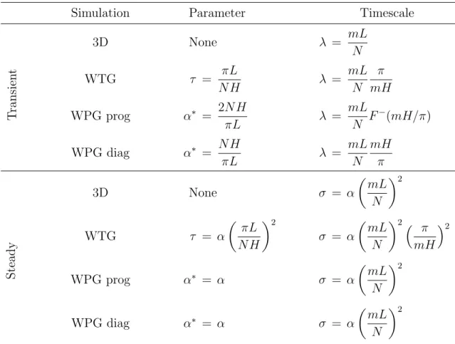
For transient solutions, which correspond to the removal of buoyancy perturbations out of a column by gravity waves, both WTG and WPG are able to generate the correct time scale for first baroclinic modes (i.e., m =π/H). But, for buoyancy perturbations withm > π/H, WTG damps the perturbations too quickly by a factor of mH/π, and both forms of WPG damp the perturbations too slowly by a similar factor (2mH/π for prognostic WPG,mH/π for diagnostic WPG). The top rows of Table 2 summarize these transient timescales.
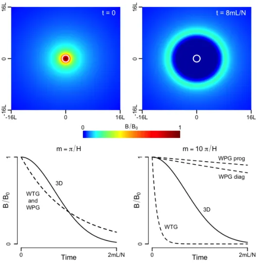
This behavior can be illustrated with the 3D solution given by (3). The top row of Figure 1 gives plan views of B/B0 from this solution atz =π/2m and two different times,
t = 0 and t = 8mL/N. The white circles outline a column of radius L. The solid curve in the lower-left panel of Figure 1 plots B/B0 at r = 0 as a function of time; as expected,
the buoyancy in the column decays on a timescale of mL/N. For the first baroclinic mode (i.e., m = π/H), WTG, prognostic WPG, and diagnostic WPG all predict an exponential decay on that timescale, which is plotted as the dashed line. The bottom-right panel shows
the decay of buoyancy for a highly baroclinic mode of m = 10π/H. Again, the buoyancy in 3D decays on a timescale of mL/N. The WTG solution, however, decays ten times too quickly. The solution in prognostic WPG decays twenty times too slowly, while the solution in diagnostic WPG decays ten times too slowly. Therefore, it is not obvious from the timescales alone that WPG would be any better at modeling transients than WTG, but other considerations, discussed below, do give such an indication.
b. Magnitude of steady-state buoyancy
As we have seen in the previous sections, a constant sinusoidal heating Q leads to a constant sinusoidal buoyancy B whose magnitude is related to that of Q by a timescale σ. These timescales are summarized in the bottom rows of Table 2. When Qis first-baroclinic (i.e., m= π/H), WTG and WPG both predict the correct magnitude of B. For sinusoidal Q with m > π/H, both prognostic and diagnostic WPG continue to predict the correct magnitude for B, but WTG predicts a buoyancy that is too small by a factor of (π/mH)2.
This underestimation by WTG of the buoyancy may lead to errors when WTG is used in a cloud-resolving model with moist convection. To see why, let us consider an atmosphere with a Rayleigh damping timescale of 1/α= 1 day and a second-baroclinic convective heating corresponding to a rain rate of 1 mm day−1 over a horizontal lengthscale of 4000 km. This
heating is comparable to the magnitude (Figure 6, Lin et al. 2004) and width (e.g., Figure 7b, Zhang 2005) of the stratiform convective heating at the peak of the MJO cycle. Using m = 2π/(15 km) and N = 0.01 1/s, equation (8) from the full three-dimensional theory gives σ3D = 4 days. A precipitation rate of 1 mm day−1 corresponds to a local heating rate
Qof at least a few tenths of Kelvin per day. Therefore, by relationB =σ3DQfrom equation
(7), this heating should generate a steady, positive, virtual temperature anomaly of at least 1 K. This matches well the magnitude of the upper-tropospheric temperature anomaly during the active phase of the MJO (Figure 7b, Zhang 2005), although rotational effects are also likely responsible for much of the observed structure.
Since a virtual temperature anomaly of 1 K is comparable to the virtual temperature excess of tropical convection, this temperature anomaly may significantly reduce cloud buoy-ancies, thereby keeping convective mass fluxes in check. WTG, however, underestimates this effect. WTG produces a second-baroclinic buoyancy anomaly that is too small by a factor of four, so convective mass fluxes are insufficientaly throttled. This may contribute to con-vective mass fluxes in WTG that are too top-heavy.
c. Shape of the buoyancy
In 3D, steady-state B and Q are related by ∇2B = α
N2∂ 2
zQ .
In WPG, B and Q are related by
B = −αL 2 N2 ∂ 2 zQ . (27) In both equations, B ∼ −∂2
zQ, which tends to colocate a peak in B with the peak in Q,
of positive heating will lead to positive buoyancy at the center of the heating, but negative buoyancy just below and above the heating. This corresponds to the adiabatic cooling of air that is drawn up into, and later up out of, the region of maximum heating by continuity. On the other hand, WTG specifies B as proportional to Q instead of ∂2
zQ, which can lead
to a qualitatively erroneous buoyancy profile.
Take, for example, the following 3D heating distribution, Q = Q0 1− r 2 4L2 exp − r 2 4L2 − (z−H/2)2 2σ2 z . (28)
The full, 3D, steady-state solution to this heating is B = α N2 L2 σ4 z σz2−(z−H/2)2Q0exp − r 2 4L2 − (z−H/2)2 2σ2 z . (29)
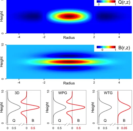
This solution is shown in the top two rows of Figure 2. When the Q distribution in (28) is restricted to r = 0 and plugged into the WPG equations, the solution we get is (29) evaluated at r = 0. The WTG solution, however, is
B = π
2αL2
N2H2Q .
The 3D solution at r = 0, the WPG solution, and the WTG solution are shown in the bottom row of Figure 2. Despite the fact that all three cases agree on the vertical velocity in response to a steady external heating (they all predict w=Q/N2, as seen from equations 1d, 9b, 15c, and 21c), only WPG matches the buoyancy profile found in the 3D solution. In WTG, the buoyancy profile has the wrong shape and a magnitude that is far too small. When moist convection is present, it is possible that these errors in the WTG buoyancy profile could feed back on the convective heating Q and significantly alter the steady-state solution.
Upon integrating equation (27) in height, we see that a steady-state column with an isolated heating has net ascent (i.e., w = Q/N2) but no net buoyancy. This falsifies the
underlying premise of the relaxed form of WTG, which is that large-scale vertical velocity is directly proportional to buoyancy. The fact that there can be no net buoyancy in a steadily ascending column is counterintuitive. To check the energetics, note that the work done by such a column is Z H 0 dz wB = − Z H 0 dzαL 2 N4 Q∂ 2 zQ = αL 2 N4 Z H 0 dz (∂zQ)2 ≥ 0.
Therefore, even with zero net buoyancy, a heated column can do work against the Rayleigh drag.
d. Nonlocal buoyancy effects
It is tempting to look at equation (2) and conclude thatB remains zero in regions where B and Qare zero. But, this would be a false inference: the differential equation for B only tells us about the time derivatives of ∂z2B, so it does not preclude nonzero time derivatives of ∂zB. To see that ∂t∂zB can be nonzero even whereB and Qare zero, we must return to
equations (1a–1e).
If we add∂xof (1a) and∂y of (1b), use continuity to replace∂xu+∂yv with∂zw, integrate
over z, and use the fact that w is zero at z = 0 andz =H, we find that
Z H
0
dz p = 0. (30)
Integrating (1c) in z and using (30) to find the integration constant, we find that
p = ρ Z z 0 dz0B −ρ1 H Z H 0 dz0 Z z0 0 dz00B , (31)
which tells us how the pressure responds to nonlocal buoyancy perturbations. This same derivation applies to the WPG equations as well.
Now, imagine that B is initially positive between heightsz1 and z2 and zero everywhere
else. Equation (31) tells us that p is negative below z1, which will drive convergence below
z1, which will lead to ascent below z1, which will lead to negative buoyancy everywhere
below z1. In this way, a localized heating produces local buoyancy perturbations, which
then produce nonlocal buoyancy perturbations. This nonlocal effect is dutifully captured by the WPG equations. In fact, the expression for ∂t∂zB can be derived from diagnostic
WPG by taking ∂z of (21c), using (21d) to replace ∂zw, using (21a) to replace δ, and then
replacing p with (31). This gives
∂t∂zB = N2 α∗L2 Z z 0 dz0B− 1 H Z H 0 dz0 Z z0 0 dz00B ! ,
which clearly shows that ∂zB initially becomes negative everywhere below a positive
buoy-ancy anomaly. We can conjecture that this effect may be important for moist convection: a buoyancy perturbation aloft can lead to lifting of the convective inhibition layer which can, in turn, trigger additional convection and additional latent heating. These nonlocal effects are not present in the WTG approximation.
7. Conclusions
This paper examines the theoretical underpinnings of methods used for parameterizing the large-scale dynamics of an atmospheric column embedded in a quiescent environment. The investigation here uses a simplified set of governing equations – the linearized, Rayleigh-damped, Boussinesq equations – that allow for analytical solutions. Beginning with 3D solutions, which serve as benchmarks, we have derived the two timescales relevant to the transient and steady-state solutions for a perturbed column. In the transient case, where a
column is initialized with a buoyancy perturbation, the relevant timescale λ is found to be the time it takes for gravity waves to propagate out of the column. In a steady state, where a column is continuously forced with an applied heating, the timescale σ that relates the buoyancy perturbation to the heating source is found to be αλ2, where α is the Rayleigh
damping rate.
We have analyzed three parameterizations of the dynamical interaction between a col-umn and its environment: a weak-temperature-gradient (WTG) approximation, a prognostic weak-pressure-gradient (WPG) approximation, and a diagnostic WPG approximation. It is found that these schemes cannot simultaneously replicate the correct transient and steady-state timescales. Instead, the parameter in each scheme (τ for WTG, α∗ for WPG) must be chosen based on whether the transient behavior or steady-state behavior is of greater interest. If the parameters are chosen to capture transient behavior, higher-order verti-cal modes travel out of the column too quickly in WTG and too slowly in WPG. If the parameters are chosen to capture steady-state behavior, WPG correctly predicts the pro-file of buoyancy at all vertical scales, but WTG predicts buoyancies for higher-order vertical modes that are much too weak. It is conjectured that the buoyancy anomaly associated with upper-tropospheric stratiform heating acts to reduce deep convection. By underestimating this buoyancy anomaly, WTG generates too weak a convective throttle and, thereby, may overproduce deep convection. Therefore, it is expected that WPG, in both its prognostic and diagnostic form, will out-perform WTG in application to steady-state cloud-resolving simulations.
Several other considerations suggest that WPG may be a more accurate scheme than WTG. First, WPG can be derived from the governing equations by replacing the Laplacian of pressure by a finite-difference approximation. WTG, on the other hand, cannot be so easily derived; instead, it relies on the premise that buoyancy perturbations are eliminated by large-scale dynamics on a fixed timescale (finite for the relaxed form of WTG, zero for strict WTG). Second, the 3D equations show that a vertically isolated heating causes a column to ascend even though the column maintains zero net buoyancy. This behavior is perfectly captured by WPG, but cannot be captured by WTG, which requires negatively buoyant air to sink. Third, the 3D equations predict adiabatic lifting of air underneath an initial positive buoyancy anomaly. The WPG equations correctly capture this behavior, but the WTG equations cannot because they require that neutrally buoyant air have zero vertical velocity. It is conjectured that this nonlocal effect of buoyancy may be important for the adiabatic lifting of convective inhibition layers. These implications are further evaluated by Romps (2012) using cloud-resolving simulations.
Acknowledgments
This work was supported by the Laboratory Directed Research and Development Pro-gram of Lawrence Berkeley National Laboratory under U.S. Department of Energy Contract No. DE-AC02-05CH11231. Thanks are due to David Raymond and two anonymous review-ers for their feedback on the manuscript.
Appendix: Compressible WPG
The extension of prognostic WPG to a compressible atmosphere is straightforward. In a cloud-resolving model (CRM) that solves fully compressible equations, the continuity equa-tion can be supplemented with a mass source −ρδ, whereδ(z, t) is evolved according to the following prognostic equation:
∂tδ(z, t) =
p(z, t)−p0(z)
ρ(z, t)L2 −α
∗(z)δ(z, t). (32)
Here, the dependence of variables on height and time has been made explicit. The variables ρ and p are the horizontally averaged profiles of density and pressure in the CRM. The profile p0 is the reference pressure of the environment in which we imagine the CRM to be
immersed. The length scaleLis the characteristic length over which we imagine atmospheric conditions transition from those represented by the cloud-resolving model to those in the reference environment. Note that Lcan be different from the size of the CRM domain. The coefficient α∗ can be a function of height in general; like L, it is an input parameter to the WPG method. The diagnostic version of WPG in a fully compressible CRM is simply
δ(z, t) = p(z, t)−p0(z)
α∗(z)ρ(z, t)L2 . (33)
For an anelastic model, we must make some approximations to be consistent with the anelastic framework. Let ˆρ(z) be the density profile used by the CRM’s continuity equation [i.e., ∇ ·~ ( ˆρ~u) = 0]. Using ˆρ for the density except where it multiplies g, the anelastic WPG equations are ∂tδ(z, t) = p(z, t)−p0(z) ˆ ρ(z)L2 −α ∗ (z)δ(z, t) (34) ∂zp(z, t) = −ρ(z, t)g (35) ∂z ˆ ρ(z)w(z, t) + ˆρ(z)δ(z, t) = 0. (36)
Here, ρ is the horizontally averaged density, including all temperature and virtual effects, i.e., ρ= ˆρ(1 +B/g), where B is the local buoyancy.
We are not yet done because we need to use boundary conditions to complete the defini-tion of p(z, t). Using (36) to replace the δ on the left-hand side of (34) gives
−∂t∂z( ˆρw) =
p−p0
L2 −ραˆ
∗δ .
Integrating in height from the surface (z = 0) to the model top (z =H) and using the fact that w= 0 at z = 0 andz =H, we get
Z H 0 dz(p−p0) = L2 Z H 0 dzραˆ ∗δ .
Adding ∂zp0 = −ρ0g (where p0 and ρ0 are the WPG reference pressure and density, which
are in hydrostatic balance by assumption) to (35) and integrating in height from 0 to z gives p−p0 = −
Z z
0
where C is an integration constant. Integrating this equation over height from 0 to H, we can identify C with the help of the previous equation. This gives
p−p0 = − Z z 0 dz0(ρ−ρ0)g+ 1 H Z H 0 dz0 Z z0 0 dz00(ρ−ρ0)g+ L2 H Z H 0 dz0ραˆ ∗δ . Substituting into (34) gives the anelastic version of prognostic WPG,
∂tδ = − g ˆ ρL2 Z z 0 dz0(ρ−ρ0) + g ˆ ρL2 1 H Z H 0 dz0 Z z0 0 dz00(ρ−ρ0)−α∗δ+ 1 ˆ ρH Z H 0 dz0ραˆ ∗δ . (37) It is straightforward to confirm that
Z H
0
dz0ρ ∂ˆ tδ = 0,
which guarantees that the vertical velocity at z = 0 andz =H remains zero. The diagnostic equations are
0 = p(z, t)−p0(z) ˆ ρ(z)L2 −α ∗ (z)δ(z, t) (38) ∂zp(z, t) = −ρ(z, t)g (39) ∂z ˆ ρ(z)w(z, t)+ ˆρ(z)δ(z, t) = 0. (40)
Multiplying (38) by ˆρ/α∗ and using (40) gives p−p0
α∗L2 +∂z( ˆρw) = 0.
Integrating in height from z = 0 to z =H gives
Z H
0
dz p−p0
α∗L2 = 0.
Adding ∂zp0 =−ρ0g to (39) and integrating in height from 0 to z gives
p−p0 = −
Z z
0
dz0(ρ−ρ0)g+C ,
where C is an integration constant. Dividing by α∗ and integrating over height from 0 to H, we can identify C with the help of the previous equation. This gives
p−p0 = − Z z 0 dz0(ρ−ρ0)g+ 1 RH 0 dz(1/α ∗) Z H 0 dz0 1 α∗ Z z0 0 dz00(ρ−ρ0)g .
Substituting into (38) gives the anelastic version of diagnostic WPG,
δ = g α∗ρLˆ 2 " − Z z 0 dz0(ρ−ρ0) + 1 RH 0 dz(1/α ∗) Z H 0 dz0 1 α∗ Z z0 0 dz00(ρ−ρ0) # . (41) Again, it is straightforward to confirm that
Z H
0
dz0ρ δˆ = 0, as desired.
REFERENCES
Blossey, P. N., C. S. Bretherton, and M. C. Wyant, 2009: Subtropical low cloud response to a warmer climate in a superparameterized climate model. Part II: Column modeling with a cloud resolving model. Journal of Advances in Modeling Earth Systems,1.
Caldwell, P. and C. S. Bretherton, 2009: Response of a subtropical stratocumulus-capped mixed layer to climate and aerosol changes. Journal of Climate,22 (1), 20–38.
Holton, J. R., 1973: A one-dimensional cumulus model including pressure perturba-tions.Monthly Weather Review,101 (3), 201–205, doi:10.1175/1520-0493(1973)101h0201: AOCMIPi2.3.CO;2, URL http://dx.doi.org/10.1175/1520-0493(1973)101<0201: AOCMIP>2.3.CO;2.
Kuang, Z., 2008: Modeling the interaction between cumulus convection and linear gravity waves using a limited-domain cloud system–resolving model. Journal of the Atmospheric Sciences, 65 (2), 576–591.
Kuang, Z., 2011: The wavelength dependence of the gross moist stability and the scale selec-tion in the instability of column-integrated moist static energy.Journal of the Atmospheric Sciences, 68 (1), 61–74.
Lin, J., B. Mapes, M. Zhang, and M. Newman, 2004: Stratiform precipitation, vertical heating profiles, and the Madden-Julian Oscillation.Journal of the Atmospheric Sciences,
61 (3), 296–309.
Nilsson, J. and K. A. Emanuel, 1999: Equilbrium atmospheres of a two-column radiative-convective model.Quarterly Journal of the Royal Meteorological Society,125 (558), 2239– 2264.
Raymond, D. J., 2007: Testing a cumulus parametrization with a cumulus ensemble model in weak-temperature-gradient mode. Quarterly Journal of the Royal Meteorological Society,
133 (626), 1073–1085.
Raymond, D. J. and X. Zeng, 2000: Instability and large-scale circulations in a two-column model of the tropical troposphere. Quarterly Journal of the Royal Meteorological Society,
126 (570), 3117–3135.
Raymond, D. J. and X. Zeng, 2005: Modelling tropical atmospheric convection in the con-text of the weak temperature gradient approximation. Quarterly Journel of the Royal Meteorological Society,131 (608), 1301–1320.
Romps, D. M., 2012: Numerical tests of the weak pressure gradient approximation.Journal of the Atmospheric Sciences, in review.
Sessions, S. L., S. Sugaya, D. J. Raymond, and A. H. Sobel, 2010: Multiple equilibria in a cloud-resolving model using the weak temperature gradient approximation. Journal of Geophysical Research, 115, D12 110.
Shaevitz, D. A. and A. H. Sobel, 2004: Implementing the weak temperature gradient ap-proximation with full vertical structure. Monthly Weather Review,132 (2), 662–669. Sobel, A. H. and C. S. Bretherton, 2000: Modeling tropical precipitation in a single column.
Journal of Climate,13 (24), 4378–4392.
Wang, S. and A. H. Sobel, 2011: Response of convection to relative sea surface temperature: Cloud-resolving simulations in two and three dimensions.Journal of Geophysical Research,
116, D11 119, doi:doi:10.1029/2010JD015347.
Wang, S. and A. H. Sobel, 2012: Impact of imposed drying on deep convection in a cloud-resolving model. Journal of Geophysical Research – Atmospheres, in review.
List of Tables
1 Variations of WPG in the literature. In the first column, a “V” denotes that the momentum damping is given by an effective viscosity and an “R” denotes a Rayleigh damping. The second column specifies whether or not the scheme uses a prognostic equation for the divergence, and the third column specifies whether or not the Coriolis force is included. 18 2 The timescales for transient and steady solutions in the linear Boussinesq
equations in 3D or as modeled using WTG, prognostic WPG, or diagnostic
Viscosity/Rayleigh/None Prognostic? Coriolis?
Holton (1973) V Y N
Nilsson and Emanuel (1999) V Y N
Raymond and Zeng (2000) R N N
Shaevitz and Sobel (2004) V, none above 800 mb Y N
Kuang (2008) R Y N
Caldwell and Bretherton (2009) none N Y
Blossey et al. (2009) R N Y
Kuang (2011) R N N
Table 1. Variations of WPG in the literature. In the first column, a “V” denotes that
the momentum damping is given by an effective viscosity and an “R” denotes a Rayleigh damping. The second column specifies whether or not the scheme uses a prognostic equation for the divergence, and the third column specifies whether or not the Coriolis force is included.
Simulation Parameter Timescale T ransien t 3D None λ = mL N WTG τ = πL N H λ = mL N π mH WPG prog α∗ = 2N H πL λ = mL N F − (mH/π) WPG diag α∗ = N H πL λ = mL N mH π Steady 3D None σ = α mL N 2 WTG τ = α πL N H 2 σ = α mL N 2 π mH 2 WPG prog α∗ = α σ = α mL N 2 WPG diag α∗ = α σ = α mL N 2
Table2. The timescales for transient and steady solutions in the linear Boussinesq equations
List of Figures
1 The top row displays B/B0 from equation (3) plotted on the x-y plane at
z = π/2m for two times: t = 0 (upper left) and t = 8mL/N (upper right). The white circle denotes the column within r = L. The bottom row shows the temporal evolution of the buoyancy at r = 0 and z = π/2m for the 3D solution (solid) and the WTG and WPG solutions (dashed) for two values of m: m=π/H (lower left) and m= 10π/H (lower right). 21 2 The top two rows display the three-dimensional solution given by equations
(28) and (29) with H = 10 and Q0 = L = σz = N = m = α = 1. The
bottom-left panel shows the profiles of Q (black) and B (red) from the 3D solution atr = 0. The next two panels show the buoyancy generated by WPG and WTG in response to the same heating profile. 22
Fig. 1. The top row displaysB/B0 from equation (3) plotted on thex-yplane atz =π/2m
for two times: t = 0 (upper left) and t = 8mL/N (upper right). The white circle denotes the column within r=L. The bottom row shows the temporal evolution of the buoyancy at r = 0 andz =π/2m for the 3D solution (solid) and the WTG and WPG solutions (dashed) for two values of m: m=π/H (lower left) andm= 10π/H (lower right).
Fig. 2. The top two rows display the three-dimensional solution given by equations (28)
and (29) with H = 10 and Q0 =L =σz = N = m = α = 1. The bottom-left panel shows
the profiles of Q (black) and B (red) from the 3D solution at r = 0. The next two panels show the buoyancy generated by WPG and WTG in response to the same heating profile.