Applied Time Series Analysis Part I

Applied Time Series Analysis — Part I

Robert M. Kunst

University of Vienna

and

Institute for Advanced Studies Vienna

October 3, 2009

1

Introduction and overview

1.1

What is ‘econometric time-series analysis’ ?

Time-series analysis is a field of statistics. There are, however, indications that a specifically econometric time-series analysis is developing. Good ex-amples are the books byHamilton(1994) and byL¨utkepohl(2005). This development reflects the typical features of economics data as well as a certain tradition of approaches that is specific to the economic science.

Economic textbooks often maintain that economics is a non-experimental science, as it typically considers observational data sets that cannot be gen-erated by repeated experiments, i.e. samples cannot be extended. If samples are seen as results of experiments, this means that the experiments of eco-nomics are non-repeatable. Compared with experimental sciences, ecoeco-nomics therefore lacks an important tool of model evaluation. However, economics is not the only non-experimental science. Most examples shown in time-series texts are non-experimental, or at least the repetition of experiments would incur high costs (for example, sunspots, accidental deaths, glacier river water).

Typical macroeconomic time series are short and come in annual, quar-terly, or monthly measurements. Many variables show characteristic growth trends. The search for an adequate treatment of such trends has inspired the development of time-series techniques that are tuned to trending data, such as unit roots and co-integration. Some of these methods are almost exclusively applied to economics data.

In finance, time-series analysis plays an important role. Typical financial time series come at high frequencies—for example, daily or intra-daily—and have large sample size. This permits the application of methods that empha-size the identification of higher moments, of conditional heteroskedasticity (ARCH), nonlinear features, and statistical distributions. Some of these methods are also applied in technical sciences, while they are not well suited to macroeconomic variables. These points concern the nature of the data. Additionally, each science has its own tradition in its perception of data information.

Firstly, it is a tradition of economics to make up for a lack of data in-formation by an increased emphasis on theory. In other words, economics tends to acknowledge the primacy of theory. This attitude implies that the role of data information is generally secondary and that the typical model is theory-driven rather than data-driven. Also, economists and statisticians use different concepts of a model. An economic model is a ‘global’ concept that targets an explanation of all observed effects inclusive of the motivation of economic agents. Such a global concept is seen as a valid model even when it fails to specify all functional relations. By contrast, a statistical (and also a time-series analytical) model is a statistical, dynamic, parametric mecha-nism for the generation of data, without any need to depict or justify the motivation for the agents’ action and reaction.

Second, economics is typically convinced that all structures are ever-changing and never time-constant. For this reason, some economists even re-ject the usage of any data analysis as a sensible means of reaching substance-matter conclusions. If one followed this radical route, time-series analysis would become useless for economics. However, any assumption of time con-stancy in a time-series model is to be seen as a working hypothesis only. Time constancy of the statistical model does not necessarily preclude non-constancy of structures in the economic model.

1.2

What is time-series analysis in general?

Time-series analysis investigates sequences of observations on a variable that have been measured at regularly recurring time points. It aims at finding dy-namic regularities that may enable forecasting future observations (beyond the sample end) or even controlling the variable (compare the title of the book by Box & Jenkins). Sometimes, by comparing time-series structures and theoretical models, time-series analysis helps in establishing evidence on theories. In the jargon of time-series analysis, such a structure is called a ‘data-generating process’ (DGP). The correct interpretation of this term is difficult. It is not guaranteed and it even appears unlikely that any simple

stochastic process exists that indeed has generated the data. If such a pro-cess exists, then it must be a very complex object, far beyond our available means. On the other hand, one may imagine myriads of processes thatcould have generated a finite sequence of numbers. Thus, that would be a very weak concept. It is maybe preferable to view the DGP as a process, which is

conceivable as an actual data-generating mechanism, which describes essen-tial structures in the observed data, and which can be utilized for prediction, for example. Some authors recommend restricting the usage of the term ‘DGP’ to situations, where data are really simulated according to an ex-perimental design from a known process. On the whole, we will follow this recommendation.

Examples for economic time series are: the Austrian GDP, the Dow-Jones index, the Swedish unemployment rate. Examples for non-economic time series are: the winning team in the Austrian football league (one annual measurement, value is a member of a set of football teams), the air tempera-ture at Hohe Warte Vienna, the wind speed at the south pole, the vote share of a political party in elections for the Vienna municipality (sometimes irreg-ular time intervals due to early elections); daily personal data: start/end of breakfast, number of cigarettes smoked etc.

Figure 1: Population of the USA at ten-year intervals 1790–1990 (from

1950 1955 1960 1965 1970 1975 1980 3500 4000 4500 5000 5500 6000

Figure 2: Strikes in the USA, 1951–1980 (from Brockwell&Davis, p.4). The textbook byBrockwell & Davis(1987, B&D; also 2002) provides some typical examples together with their graphic representation. Most of them are non-economic variables. In detail we see: an alternating electrical current measured at a resistor in a pure sine wave; observations on the U.S. population measured at ten-year intervals 1790–1980 (our Figure 1); the number of strikes in the U.S. as annual data 1951–1980 (our Figure 2); the victorious league in an annual contest between the champions of the two major U.S. baseball leagues 1933–1980 with discrete values (either National League or American League); the famous cyclical series of sunspots as annual data 1770–1869, which was compiled by the Swiss astronomers Wolf and W¨olfer (our Figure 3); a monthly series on accidental deaths in the USA 1973–1978 (our Figure 4). Figure 7 shows a typical quarterly time series from the Austrian economy, the index of industrial production.

We name three approaches to time-series analysis (time series analysis): 1. pre-classical and model-free: fitting of curves to data series,exponential smoothing (extrapolation); concept should not be discarded too easily as simplistic, as it was used in the famous studies by Malthus or by Meadows, for example;

1780 1800 1820 1840 1860

0

50

100

150

Figure 3: The Wolf&W¨olfer sunspot numbers, 1770–1869 (from Brock-well&Davis, p.6).

2. linear stochastic models, based on the sample autocovariances cov(Xt, Xt−j): the methods of Box & Jenkins (1976, re-edited as Box, Jenkins & Reinsel, 1994); forecasts are model-based extrapo-lations of the past;

3. focus on cycles and periodicities (e.g. business cycle): spectral anal-ysis, Fourier approximation, frequency domain; often this seemingly different approach yields models that are very similar to 2].

In the following, the focus will be on approach 2], which dominates the other paradigms in current academic time-series analysis, as it is represented in its main journal Journal of Time Series Analysis. A particularly im-portant recent extension is nonlinear time-series analysis (see Granger & Ter¨asvirta, 1993,Priestley, 1987,Tong, 1990, Fan & Yao, 2003).

Gourieroux and Monfort (1997) provide an alternative

classifica-tion. They distinguish the statistical and time-series analytic approach (they call it autopredictive), regression analysis (explanatory), and decomposition (adjustment) methods. The main characteristic of the first class is its aim to explain the present by the past (of one variable, i.e. univariate, or of several

1973 1974 1975 1976 1977 1978 7000 8000 9000 10000 11000

Figure 4: Monthly accidental deaths in the USA, 1973–1978 (from Brock-well&Davis, p.7).

variables, i.e. multivariate). By contrast, regression-analytic procedures use one or more conditioning reference variables, which may be controllable ‘ex-ogenously’ and which influence the dependent variable(s). Then, traditional time-series analysis may be invoked for the exogenous variables. The third class has its separate, very active community (for example, see Harvey, 1992). Technically, decomposition methods are often equivalent to the first class.

History: ‘The analysis of time series is one of the oldest activities of scientific man’ (Wayne Fuller, 1996, p.1) [Homo sapiens ssp. scientificus]

1.3

Stochastic processes

A (discrete) stochastic process is a sequence of random variables (X1, X2, . . .)

that is defined on a common probability space. It becomes a time-series process if the index sequence 1,2, . . . can be identified with—typically equidistant—time points. The term ‘time series’ denotes a specific

realiza-tion of the process, i.e. a ‘trajectory’1_{, or more commonly a finite segment}

of a trajectory. If (Xt) denotes a process, then (Xt(ω)) for fixed ω defines a

time series. Hence, a time series is—in simple terms—nothing more than a few (say, T) numbers, which can be plotted against the time axis and which can be joined by a curve. By contrast, a process is an object that can be represented symbolically only (for example, by a sequence of density curves). There is a formal distinction between the finitely indexed time series and the theoretically infinite trajectory. It is a customary abstraction, however, that any stochastic process stretches into the distant future (T _{→ ∞}), even if by definition one may never observe more than a limited time segment of a variable. For example, it appears difficult to concatenate macroeconomic variables such as the German unemployment rate, observed from the end of World war II to the German re-unification, with earlier or later observations. Certainly, however, all observed time series can possibly exist only until the heat death of the universe that is predicted by some physicists.

Some authors insist that a stochastic process is not merely a ‘sequence of random numbers that is written down one by one’. In order to understand the concept of a process, it is of particular importance that all joint distributions of n–tuples like (Xt, Xt+j, Xt+k) are always properly defined.

A stochastic process belongs in the realm of time-series analysis, whenever the sequence index can be interpreted as ‘time’. If it has an interpretation as a spatial coordinate, it is a spatial process. Even mixed forms of space-time processes have been often considered recently (inspired by observed panel data, for example annual data for tourism in Austrian provinces 1960–2000). If time—at least conceptually—can be condensed such that the process becomes observable continually, then (Xt) becomes a time-continuous

pro-cess. This is a sensible abstraction for few economic variables only (for exam-ple, some stock-market prices). Continuous time is a lively field of research but it is outside of our scope here (for example, see Bergstrom, 1990). A typical problem is the approximation of a theoretical time-continuous pro-cess by an observable time-discrete propro-cess and the possible equivalence of properties across the limit operation.

Formally, a stochastic process is defined as measurable mapping from a probability space (Ω,_A, P) into a sequence space. Note that the sequence space itself is formally defined as a set of mappings from an index set (for example, natural numbers) into a reasonable codomain (for example, real numbers or a discrete set of characteristics). Anyway, this definition may

1

Statistics differentiates between a random variable (‘the principle of rolling a fair die’) and a specific realization (‘4’). In the case of a process, the realization is a sequence o numbers.

not be immediately accessible to many. Examples of stochastic processes:

1. rolling a die T times. The observed T–sequence (e.g., 1,2,4,2,2,6, . . . ,3) is a time series. The index set of the se-quence is _{1, . . . , T_}, the probability space is rich enough to contain all events (for example, there are well-defined probabilities that all T

numbers are even or that no 6 appears in the time series). Domain of values (codomain) are the numbers from 1 to 6.

2. tossing a coin T times. Like 1] but the codomain is (heads, tails) or (0,1). In 1] and 2], members of the sequence are independent.

3. numbers generated by a random-number generator. If the generator is known, this is in principle not a stochastic process, as specific se-quences have probability one for a given starting value and all thus generated time series are identical. In practice, however, the time se-ries behaves almost like independent random numbers, i.e. like 1] or 2]. The codomain of a generator for normal random numbers is in prin-ciple finite (a set of machine numbers with finite precision), although it is usually identified with the real numbers. Usually, the probabil-ity space contains all ‘Borel’ sets. This requires that events such as ‘2< xt <3.45 holds exactly 10 times in the sequence’ must have a P,

and also all intersections, unions etc.

4. The problem of the drunk man wandering aimlessly down a street with two bars, who could be seen as taking a step to the right if a tossed coin shows tails and a step to the left if it shows heads. The drunk’s location can be seen as a stochastic process. Of course, the present location depends on the preceding realization. This is an example of a so-called random walk (RW), which for a finite distance to the bars becomes a stopped RW. The codomain are all multiples of step sizes, measured from the point of departure.

In analogy to common practice in econometrics, the observed realization of the time series is viewed as one of (typically infinitely) many virtual re-alities. This concept is necessary in order to create a statistical framework and to formalize the problem of prediction. An alternative paradigm would be the concept of chaos, i.e. a deterministically generated time series, whose DGP is so complex that it behaves like the trajectory of a stochastic process2_.

2

A process or a component of a process is calleddeterministic_{if its trajectory is known}

(determined) exactly at the time point when it is started. Sometimes, the terms ‘deter-ministic’ and ‘non-stochastic’ are equated, which is slightly sloppy and misleading.

Actually, such a DGP appears in example 3]. Another paradigm, Bayesian statistics, rejects the idea of a true DGP and views all statistical models as created by continuous interaction of the observer’s constructions and the data. Often, Bayesian methods yield results that are similar to traditional ones, while the utilized procedures are considerably more complex.

1.4

Stationarity

Even if the stochastic process follows a normal distribution, still T observa-tions of a time series would require estimating T +T(T + 1)/2 parameters. This is impossible. However, if distributions are assumed as time-constant, the number of free parameters declines palpably to T + 1. The assumption of further plausible restrictions allows another reduction of the parameter dimension, such that finally efficient estimation becomes feasible. The time-constancy of the statistical distribution (not only of the marginal univariate, but also of all multivariate and hence of all conditional distributions) is called

stationarity.

Examples 1],2] describe stationary processes, 3] at least conceptually, but not 4]. 1] and 2] are rather special cases, however, due to their independent realizations. An example of a stationary, temporally correlated process is the following:

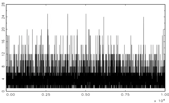
Example: Rolling a die with a bonus. Write down the number of dots on the top face. If it is a 6, the number that comes up at the next roll is doubled, if it is another 6, it is tripled etc. It is easily seen that all multiples of the numbers 1 to 6 can occur. In the univariate marginal distribution, however, the number 18 will be much less probable than 2, for example. Hoping that the marginal distribution does not degenerate (i.e. that it does not ‘escape’ to _∞), our generating law yields a stationary process, which is no more temporally independent.

In the example ‘rolling a die with a bonus’, we of course do not have a nor-mal distribution. The nornor-mal distribution has the technical advantage that it is described completely by its first two moments, the mean and the variance (in multivariate applications the mean vector and the variance matrix). We may consider simplifying the work by postulating:

Postulate A: The process is stationary and normally distributed

Unfortunately, this is a very restrictive assumption. It is more acceptable to work with a similar concept that also allows restricting attention to the first and second moments. That concept is rooted in the theory ofL2 _{spaces. By}

just narrowing our vision to the information of the first two moments, we can build up a powerful theory of time series that admits potential changes of higher moments over time.

Figure 5: Simulated time series for the example ‘rolling a die with a bonus’.

Postulate B: The process has time-constant first and second moments Postulate B defines the so-called covariance stationarity or weak stationarity. For most results and techniques of time-series analysis, this concept suffices. It is so important that we repeat it in formal terms:

EXt = µ ∀t

varXt = σ2 ∀t

cov(Xt, Xt−h) = cov(Xs, Xs−h) ∀t, s, h (1)

An exception to the ubiquitous dominance of covariance stationarity is the analysis of financial markets that requires the modelling of higher moments.

Example. ‘alternating nuisance’: (Xt) is generated by drawing for all

even t from standard Gaussian N(0,1) random numbers, for all odd t from Laplace random numbers scaled to unit variance. The process is not station-ary but weakly stationstation-ary (mean and variance are constant, all covariances are zero).

Example. ‘absurd exception’: (Xt) is drawn from Cauchy random

num-bers. The process is certainly stationary but not weakly stationary, as first and second moments do not exist.

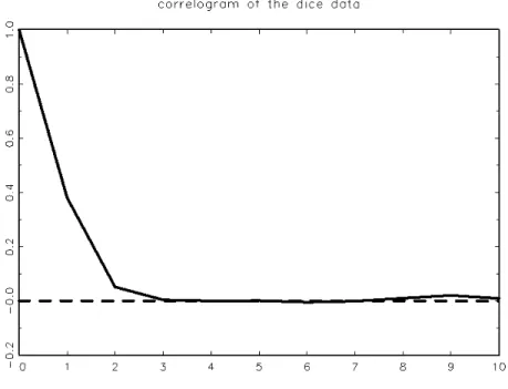
Figure 6: Empirical ACF (correlogram) for the data shown as Figure 5. Usually, however, stationarity implies weak stationarity. Stationarity per se is also called ‘strict stationarity’ to differentiate it from covariance sta-tionarity.

Summary: Working with weakly stationary processes can be interpreted as viewing all processes as strictly stationary but restricting focus to the co-variance structure; or as viewing actual processes as non-stationary with time-changing higher moments. In a normally distributed world both defini-tions and interpretadefini-tions coincide.

Example: Sequential rolls of a die or normally distributed (true) random numbers yield processes, whose variance σ2 _{is constant, whose mean is}

con-stant (for normally distributed random numbers typically 0, for the rolled die 3.5), and whose temporal (serial) correlation is zero (corr (Xt, Xt+i) =

0 _∀i₆= 0). This very special stationary process, in a sense the most prim-itive, most elementary and most important of all covariance-stationary pro-cesses, is called white noise (wn). In the following,εtalways denotes a white

noise.

Example: The definition of a ‘white noise’ determines only the first- and second-moment properties. It is customary to require Eεt= 0. The following

law defines a wn. Start from an arbitrary X0. If we observe Xt > 0, draw

from a uniform distribution U(₋1/√3,1/√3). This process is even strictly stationary, while it is not temporally independent. It is easily seen that it is a wn. A temporally independent process with time-constant distribution is often indicated by the abbreviationiid(independentidenticallydistributed).

Repetition: white noise is a process (εt) that obeys Eεt = 0,Eε2t =σ2

(positive and finite), Eεtεt+i = 0 ∀i6= 0. Such a process is not necessarily

strictly stationary and not necessarily serially independent. iidis a process of serially independent draws from the same probability distribution. An iid– process is always strictly stationary but it does not necessarily have finite variance. Assumptions regarding the mean or location of random variables (such as Eεt = 0) are in principle arbitrary.

Examples ‘alternating nuisance’ and ‘absurd exception’ revisited: alter-nating nuisance is a wn–process, certainly not iid. Absurd exception is iid, though not white noise. Note the subtle differences. Alternating nuisance is wn but not strictly stationary, hence it cannot be iid. The example with conditional drawings defines a wnthat is even strictly stationary, whose de-pendence via higher moments violate the iid–property.

In the following, the word ‘stationary’ will always refer to covariance stationarity.

1.5

Autocorrelation function ACF

An important tool for the analysis of covariance-stationary processes is the autocorrelation function (ACF) or, alternatively, the autocovariance function (with some authors ACVF). The autocorrelation function is more common. Using the notation EXt=µ, it is defined by

ρ(h) = E{(Xt−µ)(Xt+h−µ)} E_{(Xt−µ)2}

, (2)

which for µ= 0 simplifies to

ρ(h) = E(XtXt+h) EX2

t

.

The numerator of (2), cov (Xt, Xt+h) as a function of h, is the

autocovari-ance function and it is commonly denoted by the symbol γ(h). Because for stationary processes the denominator is constant, the only difference of ρ(.) and γ(.) is a factor γ(0) that is just the variance of the process.

Note that the formula forρ(h) really yields the correlation ofXtandXt+h,

as the traditional denominator qE(X2

tXt2+h) is simplified by the assumption

from stationarity. In principle, it makes sense to define the autocovariance function for non-stationary processes by

ρ(s, t) = p E{(Xs−EXs)(Xt−EXt)}

E_{(Xs−EXs)2}E{(Xt−EXt)2}

as a function of two arguments (e.g., in Brockwell & Davis), but such generalizations require the correct traditional denominator.

Definition (2) is tuned to stationary processes, as ρ(.) must not depend ont in the stationary case. The ACF has several other attractive properties. First we observe:

(Fuller’sTheorem1.4.2)ρ(₋h) =ρ(h) and γ(₋h) =γ(h) for covariance-stationary real-valued processes.

Remark: This property does not hold for complex-valued processes. The theorem implies that it is meaningless to evaluate the ACF for negative and positive h separately.

(ρ(0) = 1, ρ(1), ρ(2), . . .) defines a sequence of real numbers. Not every combination of numbers can occur in this sequence. The characterization of all possible sequences is achieved by (Fuller’s Theorem 1.4.1), which states that the ACF is positive semi-definite (or non-negative definite). This means that, for any finite sequence of real numbers (a1, . . . , an) and for any

corresponding sequence of natural numbers (i1, . . . , in) n X j=1 n X k=1 ajakρ(ij −ik)≥0. (3)

Settingn = 2 immediately yields the important property that_|ρ(h)_{| ≤}1, which corresponds to the interpretation as a correlation (proof as an exercise or in Fuller, p.8). For n > 2 it is less easy to interpret this condition. It is recommended to view it simply as an algebraic condition, which guaran-tees that all constructible variances are non-negative and which limits the selection of possible shapes for the ACF.

An important theoretical result is thesynthesis theorem, which states that all positive semi-definite functions (withρ(0) = 1 can occur as ACF of a stationary process. To any positive definite function one can find/construct a process that has the given function as its ACF.

Even more important is the fundamental property—whose proof relies on representation theorems—that the ACF (together with the mean µand the variance) contains all essential information on the covariance-stationary pro-cess. In other words, the sequence ρ(.) (& mean & variance) ‘characterizes’ the process. For example, the important problem of selecting the parametric

representation of the process can be based on the ACF alone. No further information that would be extractable from the data helps with this task. In a sense, processes with identical ACF are equivalent.

For example, the process ‘rolling a die with a bonus’ appears to have the ACF that is shown in Figure 6. It is easy to construct a theoretical process (even with normally distributed random errors) that has exactly the same ACF. Both processes—‘Rolling a die with a bonus’ and the synthetical process—are equivalent, although they differ with respect to many statistical properties. As long as the boundary of the so-calledL2 _{theory of}

covariance-stationary processes is not transgressed, will such differences play no role, as they cannot be ‘perceived’.

1.6

Trend and seasonality

Time-series analysis is primarily concerned with time series (and/or corre-sponding processes, according to definition) that have a time-constant co-variance structure and time-constant mean and volatility. These are called stationary. Approach # 3 in the introduction indicates that it could also be said in other words that time-series analysis is concerned with cyclical stochastic processes, whose cycles have finite amplitude and frequency but are never exactly constant. Even approach # 3 leads to the covariance-stationary processes. Many economics data series, however, do not conform to these assumptions and thus resist a direct treatment by time-series anal-ysis.

Examples:

1. B&D give as their Example 1.1 a time series of measurements of an electric current at a resistor. This could be a pure deterministic cycle. In such a process, any future observation can be predicted exactly. Also in economic examples can a specific cycle (e.g. the seasonal cycle) dom-inate to such an extent that all remaining structure becomes entirely unrecognizable.

2. Their Example 1.2 (here Figure 1) shows the population of the USA in 10–year measurements. This is a trending time series. Its mean is clearly not time-constant.

3. Their Example 1.6 (here Figure 4) shows monthly measurements of accidental deaths. This is another seasonal series. Its mean may be constant in the long run, while within the sample the accidental deaths in July appear to exceed those in February. Hence, the mean experi-ences cyclical oscillations that may have a deterministic component. If

EXtdepends on the remainder class oft, the assumption of stationarity

is violated.

4. Their Example 1.5 (here Figure 3) are the legendary sunspots. From 1800 to 1830, their volatility appears to have been lower than at other times. If this were true, σ2 _{would be not constant and stationarity}

would be violated. This interpretation, however, is not coercive. The analysis of financial time series utilizes so-called ARCH processes that are covariance stationary and whose observed volatility changes are explained by cross moments of order four.

5. Their Example 1.3 (here Figure 2) is an annual series of strikes in the USA, which appears to be extremely irregular. If mean and/or volatility change at specific break points, economists call these time points ‘structural breaks’. The adequate treatment of this feature is uncertain, even the role-model example B&D 1.3 would be diagnosed and treated differently by different time-series analysts.

In summary, one should distinguish problematic deviations from the as-sumptions (volatility changes, structural breaks) and standard deviations with adequate routine treatment (trend and seasonality).

For the trend feature, we have two basic strategies, each of which has its advocates:

1. The time series is regressed on a simple function of time, such that the residual can be viewed as ‘stationary’. Fitting curves to data used to be quite common of in the history of econometric time-series analysis, today the choice of time functions is restricted to:

(a) a linear trend function, i.e. a straight line;

(b) a quadratic trend function, i.e. a parabolic curve, but only if quadratic growth can be justified by plausibility arguments, which excludes unemployment rates, for example;

(c) an exponential trend function that conforms to case (a) after transforming the data by logarithms.

A disadvantage ofcurve fitting is that it often yields excellent resultsin sample but leads to nonsensical results if extrapolated out of sample. 2. Transforming the raw data so that the assumption of stationarity

(a) first differences xt=Xt−Xt−1, which are usually denoted by ∆X

or by _∇X;

(b) logarithmic differences xt = log(Xt/Xt−1) are first differences of

the logarithmized data;

(c) growth rates 100(Xt−Xt−1)/Xt−1 have properties similar to case

(b) and are therefore often applied to the same data sets (even though there are important conceptual differences between the two methods);

(d) seasonal differences xt = Xt − Xt−4 (4 for quarterly data, 12

for monthly data) are also denoted by ∆4 etc. These seasonal

differences remove trend and seasonality simultaneously.

The application of first differences (also called differencing) has been enjoying growing popularity in econometric time-series analysis since the publication of the book byBox & Jenkins. Compared to the more traditional trend fitting, it has different implications for the dynamic equilibria of econom(etr)ic models and for the long-run behavior of variables. These differences dominated the discussion of persistence and unit roots (around 1980–1990).

3. In particular, the empirical sections of contributions from the field of

real business cycles has seen an increasing intensity of applications of the de-trending method by Hodrick& Prescott. This procedure uses frequency-domain properties of time-series models.

For the seasonality feature, a wide variety of potential procedures is avail-able. It is recommended to consult the monographs by Hylleberg (1986) and by Ghysels & Osborn (2001). We mention the following procedures: 1. Seasonal dummies are probably the oldest technique3_{. The seasonal}

cycle is modelled as a strictly periodic deterministic process, whose specification requires 4 or 12 coefficients (without the constant, 3 or 11). This modelling concept is fully supported by most econometric software products. Following an auxiliary regression, the residuals are either viewed as stationary or the seasonal dummy variables are integrated into the modelling process. A seasonal dummy is specified as 1 in a specific month (or quarter) and is 0 otherwise.

Disadvantage: inflexible seasonal pattern, unclear interaction with trend modelling. These problems motivated the development of

3

2. Seasonal adjustment, which today commonly relies on the legendary routine ‘Census X-11’ or on one of its descendants X-12 and TRAMO-SEATS. A sophisticated sequence of smoothing and de-trending filters together with outlier adjustment and time-series model steps succeeds in ‘adjusting’ the data, i.e. in purging them from any seasonal char-acteristics, while other information—such as business cycles or trend behavior—is retained. Particularly the outlier correction and other non-linear components of the procedure are irreversible, meaning that the original data cannot be recovered from the adjusted series.

Disadvantage: Destruction of information, which may be dangerous if the true dynamics of seasonality does not correspond to the model that is implicitly assumed by the Census X-11 procedure; aliasing ef-fects spreading to non-seasonal frequencies; insufficient theoretical basis for all operations; adjusted data may reflect arbitrary manipulations. For these reasons, many time-series analysts (unlike some empirical economists; see also Box & Jenkins, 1976) recommend:

3. seasonal differences, see item (d) of ‘trend’. Seasonal differencing treats trend and seasonality alike. This methods can also be justified on statistical grounds by theoretical models and hypothesis tests (among others, see Hylleberg, Engle, Granger, Yoo, 1990, for the so-called HEGY test).

Disadvantage: seasonal variation may not be restricted enough in the HEGY model. The implied stochastic seasonal cycle admits reversals of summer/winter patterns, even in cases where this may appear implau-sible (e.g. temperature). It should be noted, however, that summer-becomes-winter actually did occur in economic time series, for example in regional tourism, where demand does not peak any more in summer but in winter due to winter sports, or in energy demand, where air conditioning causes a formerly unknown peak in summer.

4. the seasonal moving average (SMA) is actually one component of the seasonal difference operator, or in other words: SMA + first differencing = seasonal differencing.

Disadvantage: phase shift by asymmetric filtering (which also appears in seasonal differences); phase correction may be achieved by other methods of weighted averaging, see e.g. B&D methods S1 and S2. Gen-erally, method 4] is to be preferred to 3] if data do not have trends. Figure 7 shows a typical macroeconomic time series, Austrian industrial production 1962–2002. Trend and seasonality are clearly visible. In Figure

9 the operator ∆ has eliminated the trend, the seasonal cycle is clearly dis-cernible. Figure 8 shows the series after smoothing by the SMA filter, Figure 10 shows seasonal differences. It is obvious that the operator ∆4 eliminates

trend as well as seasonality.

Figure 7: Austrian industrial production 1962–2002. Quarterly data pro-vided by OECD, after logarithmic transformation.

If forecasting is the aim of the analysis, another distinctive feature of the methods may become crucial. Some procedures admit predicting the original (untransformed, ‘unfiltered’) process, while others can only be used for predicting the transformed, ideally stationary process. In particular the B&D methods S1 and S2, X-11/12, the HP filter do not allow forecasting the unadjusted variable. The B&D methods explain trends only locally (by non-parametric smoothing), the trend remains unexplained outside the sample. HP and Census destroy sample information in specific frequency bands (in the long-run band for trends and in an area around the seasonal frequencies, respectively). With regard to X-11/12, this destruction may be justified by the popular view that seasonally adjusted data are (closer to) true data. Under this assumption, of course, forecasting the seasonally adjusted data appears sufficient.

Figure 8: Seasonal moving averages of industrial production. Data filtered by 1 +B+B2_+B3_.

2

ARMA processes

It was already outlined that one of the (more or less equivalent) approaches of time-series analysis is based on the idea of describing observed time series by classes of comparatively simple processes. In other words, this modelling aims at ‘parameterizing’ the ACF, that is to find a model that approximates the empirically estimated ACF as well as possible. It can be shown (Wold’s Theorem) that every covariance-stationary process can be approximated ar-bitrarily well by so-called moving-average processes (MA). Similarly, almost every covariance-stationary process can be approximated arbitrarily well by autoregressive processes (AR). Note that ‘approximation’ always refers to a matching of theoretical and empirical ACF (second moments), while noth-ing is stated on higher moments or other stochastic properties. Finally, the ARMA process is an amalgam of its two basic elements AR and MA.

2.1

The moving-average (MA) process

The MA process directly generalizes white noise. Assume that (εt) is wn

with variance σ2_{. In the following, we will use σ}2 _{for the variance of (ε}

Figure 9: First differences of the logarithmized industrial production data (Growth rates relative to previous quarter).

while otherwise we use the detailed notation of, for example, σ2

X to denote

the variance of (Xt). Then,

Xt=εt+θεt−1 (4)

defines an MA process of order one (a ‘first-order MA process’), symbolically denoted by MA(1). The parameter θ may be any real number. This process has the following attractive property:

Property 1: The MA(1) process is covariance stationary.

To show this, we just determine the first and second moments. By using the linearity of the expectation operator and the properties of the wn (εt), it is

immediate that EXt= 0, that varXt= (1 +θ2)σ2 and that EXtXt−1 =θσ 2_.

This implies that

ρ1 =

θ

1 +θ2 , (5)

with the shorter notation ρh instead of ρ(h), which we will use in the

fol-lowing. All ρh with h >1 are clearly 0, and hence the thus defined process

is stationary. If we replace θ by 1/θ in (4) and (5), we note to our surprise that this yields the same value for ρ1. Thus, for example the MA(1)

Figure 10: Seasonal differences of the logarithmized industrial production data. Growth rates.

‘equivalent’. Their variance may be different, but the variance of εt is

un-observed. For observed data, the error variance results from θ and varX via

σ2 _{= varX/(1 +θ}2_{). We have established:}

Property 2: MA(1) processes with coefficientsθand with 1/θare equiv-alent. Therefore, one may restrict attention to the case _|θ_{| ≤}1.

This means we cannot tell whichθ out of the two has actually generated the data. If estimation yields a value θ > 1, we can replace it by 1/θ and obtain an equivalent estimate. No substance conclusions can be drawn from the fact that an estimated θ exceeds one.

What do these MA(1) processes look like? Formula (5) reveals that ρ1

is negative for θ < 0 and positive for θ > 0. The boundary case θ = 0 is of course just the wn process. This degenerate case would not be classified as a MA(1) process but as MA(0). Starting from θ = 0 in either direction, let us increase θ in its absolute value. At first, ρ1 will also increase in its

absolute value. However, autocorrelation reaches its maximum of 0.5 for

θ = 1. Property 2 states that further increases in _|θ_| imply lower values of

ρ1. This observation implies the following important property:

Property 3: The class of MA(1) processes describes all covariance-stationary processes, for which ρ1 ≤0.5 and ρi = 0 for all i >1.

Therefore, if an observed process has an estimatedρ1 >0.5 and if we can

recognize several non-zero ρi with i >1 that are either positive or negative,

then MA(1) cannot be a good model for the data-generating process.

Obviously, the next point should be MA processes of higher order. It is straight forward to define the MA(2) process by

Xt=εt+θ1εt−1+θ2εt−2, (6)

and more generally the MA(q) process by

Xt=εt+θ1εt−1+θ2εt−2+. . .+θqεt−q. (7)

Simple application of the expectations operator and exploiting its linear-ity as well as the definition of a wn yields

Property 1: MA(q) processes are always stationary. ρh = 0 for allh > q.

The autocovariances γh for h ≤ q can be expressed in the coefficients θi, in

detail:

γ1 = σ2(θ1+θ1θ2+. . .+θq−1θq)

γ2 = σ2(θ2+θ1θ3+. . .+θq−2θq)

γ3 = σ2(θ3+θ1θ4+. . .+θq−3θq)

· · ·

The structure of the formulae is clearly recognizable. It is even better recog-nizable if we set formally θ0 = 1. Then, we have generally:

γh =σ2 q−h X

i=0

θiθi+h, 0≤h≤q. (8)

For h= 0 this yields the variance formula varXt=γ0 =σ2

q

X

i=0

θ_i2 . (9)

From these formulae, the ACF evolves as

ρj = Pq−j i=0θiθi+j Pq i=0θ2i , j _≤q.

And what about Property 2 for the general MA(q) model?

Property 2: Generally, there are 2q _{different combinations of q}

param-eters _{θ1, . . . , θq}, all of which imply the same ACF and therefore define

In order to obtain a unique representation, we need the concept of a characteristic equation. According to an immediately obvious principle, we attach to any MA model

Xt =εt+θ1εt−1+. . .+θqεt−q

the characteristic polynomial, formally written in the complex variable z,

θ(z) = 1 +θ1z+. . .+θqzq.

This polynomial has for z _∈C _{exactly q zeros or ‘roots’ζ1, . . . , ζq. One can}

show that the equivalent MA processes correspond to those polynomials that are created by replacing one or more of these zeros ζj by ζ

−1

j . This implies

that there is exactly one MA process, for whichall zeros are larger or equal to one, according to their absolute value or ‘modulus’. If we convene to always choose this process, then the representation is unique.

Remark. These properties are strictly valid only if we ignore the possi-bility of multiple and unit roots. If we account for this possipossi-bility, we should say that there are at most 2q _{different equivalent representations.}

There is a reason why we do not, for example, choose the representation with all zerosless than one. The model with large zeros is the one with small coefficients and thus embeds white noise. Furthermore, one can show that an MA process can be represented as a convergent series

∞ X

j=0

φjXt−j =εt,

if and only if the roots of the characteristic polynomial are strictly greater than one. This ‘infinite AR representation’ is convenient for prediction. If it exists, the MA process is called invertible.

Hence, it is always possible to select a specific solution that fulfils the identifying restriction. Computer programs could first—utilizing non-linear optimization or comparable techniques—estimate a parameter vector, then replace it by an equivalent one that fulfils the uniqueness condition, and print out this final estimate.

For plausibility reasons, attention typically focuses exclusively on MA processes that are constructed from past εt. Such processes are also called causal, as it is usually assumed that causes precede their effects. The oppo-site would be an anticipative process that explains the past by the future. Occasionally, it makes sense to consider mixed forms. One may distinguish

by Xt= q2 X j=−q₁ θjεt−j.

All of these extensions are, of course, stationary.

What do these higher-order MA processes look like? One can show that every covariance-stationary process can be ‘represented’ as an infinite-order(!) MA process (Wold’s Theorem). The higher the MA order, the more processes can be modeled. Although according to Property 1 ‘the ACF must cut off’, this cut-off can only limit the process behavior in quite large samples (T >> q). Even limitations according to the definiteness require-ment of the ACVF —such asρ1 ≤0.5 for MA(1)—lose their importance with

increasing order p.

Figure 11: 100 observations of the process Xt=εt+εt−1+εt−2.

Figure 11 shows a segment of a trajectory from an MA(2) process with

θ1 = θ2 = 1, which even casual eyeballing may be able to tell apart from

a wn. Such examples demonstrate that higher-order MA processes tend to ‘oscillate’, which MA(1) processes cannot do. It appears difficult, however, to discern the cycles visually, the modelling of strong cyclical behavior is more easily done by AR models.

We note thatWold’s Theorem contains a special feature, as the meaning of an infinite-order MA series ∞ X j=0 θjεt−j (10)

is not immediately obvious. Such expressions must converge to become mean-ingful. One can show that ‘quadratic convergence’ of the series of coefficients suffices for this purpose, i.e.

∞ X

j=0

θ2

j <∞. (11)

In order to guarantee convergence of infinite sums of the form P

θjut−j for

autocorrelated input—withustationary but notwn—it is helpful to demand the stronger condition of ‘absolute convergence’ for the coefficients series, i.e.

∞ X

j=0

|θj|<∞. (12)

It is easy to see that absolute convergence is stronger than quadratic conver-gence of series. Consider for example the sequence 1/n. If summed up to a series, it diverges, while the sum of the squared 1/n2 _{converges to π}2_/6.

Within the boundaries of the ARMA processes and of these lecture notes, there is no difference between absolute and quadratic convergence. However, there is a cost involved in limiting attention to absolutely convergent MA(_∞) processes, as this excludes some important stationary cases. Processes with-out absolute convergence of their Wold coefficients series are said to have

long memory. It is doubtful whether they play a role in economics, although there is some evidence for long memory in interest rates and other financial series.

Summary: An MA process, constructed from a quadratically convergent coefficients sequence (θj) and white noise, is covariance stationary. If we

consider an infinite sum of weighted observations of a stationary process instead of a weighted sum of wn terms, then the thus defined process will be stationary if its sequence of coefficients is absolutely summable.

2.2

Autoregressive processes (AR)

Whereas the MA-process is formally easier to handle, to many empirical researchers the autoregressive process is more intuitive and easier to interpret. A dynamic generating law such as

can be found in many places, not only in economics. (13) defines the first-order autoregressive process, in short AR(1). We again set µ = 0. The properties of the process are determined by two parameters: the coefficient

φ and the error variance σ2_{. Forφ = 0 will the process degenerate to a wn.}

A generating law such as the difference equation (13) may have diverse interpretations. Some see a recursion starting from a given and fixed value for X1 or X0, a so-called starting value. While drawing repeatedly

uncor-related random variables εt, the recursion generates the time-series process.

The thus defined process will usually not be stationary, as the first observa-tion follows a different distribuobserva-tion from the tenth, say, which still feels the starting value strongly, and this tenth observation will again follow a different law from the 1000th. Under certain conditions, however, will the process ap-proximate a stationary one gradually. Some call this gradual approximation to a stationary steady state ‘asymptotic stationarity’.

A different interpretation is that the process (Xt) has already been active

for an infinite time span and that we just start observing it at some time point. Such a process may actually be stationary. In detail, one has the following theorem:

Property 1: The AR(1) equation (13) has a stationary solution, if and only if _|φ_|<1.

To proof and to motivate this result, we may consider some calculations. First we may substitute the right-hand side of (13) repeatedly into the left-hand side, which yields after an _∞number of substitutions:

Xt= ∞ X j=0 φj_ε t−j. (14)

This is an MA(_∞)–process with geometric and therefore (as a series) abso-lutely convergent sequence of coefficients, which certainly is stationary. By contrast, if _|φ_{| ≥} 1, then summing up will not be possible. The case φ = 1 is called the random walk, i.e. a non-stationary process. The case _|φ_| > 1 is called an explosive process. If φ = ₋1, some authors name it a random jump.

Another calculation exercise evolves from the attempt to determine the process varianceσ2

X assuming stationarity. If (Xt) is stationary, then we have

var(Xt) = var(Xt−1) and hence:

E(X_t2) = φ2E(X_t2−1) +σ 2_,

E(X_t2) = σ

2

1₋φ2. (15)

Obviously, a sensible solution is possible only if _|φ_| < 1. Thus, whereas all MA processes are stationary, some AR processes are stationary, while others

Figure 12: Trajectory of an AR(1) processXt= 0.5Xt−1+εt. A pre-sample of

50 data points guarantees that the shown process is approximately stationary. are not. We note for completeness that the stochastic difference equation (13) possesses even for _|φ_| > 1 stationary solutions, but those are antici-pative and are seen as implausible. This pecularity explains why explosive and stationary AR processes have identical ACF in finite samples (i.e. the estimated ACF or correlogram, while the theoretical ACF is undefined for explosive processes). For example, φ = 0.5 and φ = 2 in (13) yield identi-cal correlograms. Therefore, the correlogram cannot be used to determine whether the observations follow an explosive scheme.

In the following, a process will be calledstable if its scheme has a station-ary solution, such that ‘the difference equation is stable’. Thus, an AR(1) process is stable for _|φ_| < 1 but it may not be stationary. Others call such processes ‘asymptotically stationary’.

Property 2: The first-order autocorrelation of a stationary AR(1) pro-cess is simply ρ1 =φ. Generally, we have ρh =φh.

This is easy to show. It follows that the ACF of a stable AR(1) decays geometrically, in an alternating pattern if φ < 0. The empirical ACF (the correlogram) reflects these properties only approximately.

This geometric decay (in contrast to the cut-off in the ACF of an MA process) is characteristic for all AR processes. In consequence, if my

time-Figure 13: Trajectory of the random walk Xt = Xt−1 + εt, started from

X1 = 0.

series data yield an ACF with cut-off after a specific p or a hump-shaped ACF—which is often observed for quarterly data, whereρ4is more important

than ρ3—then AR(1) is probably an inadequate model for my data.

An AR(1) process does not oscillate. Thus, it is not suited for the descrip-tion of business cycles. Even when φ < 0, it does not really oscillate but it alternates or jumps with fixed periodicity, i.e. one observation is positive, the next one is negative, and so on. The properties of difference equations imply that even the most immediate generalization to second order can generate cycles of (almost) every periodicity. Processes of the form

Xt =µ+φ1Xt−1+φ2Xt−2+εt (16)

are called second-order autoregressive processes or in short AR(2). Again we set µ = 0. Then, the process—apart from σ2_{—depends on two parameters,}

the coefficients φ1 and φ2. To us, this appears to be the most reasonable

parameterization. For the determination of stationarity properties, however,

φ1andφ2 are not the ‘natural’ parameters of the model class. In consequence,

the stability or stationarity conditions become quite unwieldy for AR(2) pro-cesses. The situation deteriorates further for AR(p)–processes with largep.

Figure 14: Empirical (solid) and theoretical (dashed) ACF of the process

Xt= 0.5Xt−1+εt.

Property 1: The AR(2) process is stable if and only if (a) φ1+φ2 <1,

(b) φ1−φ2 >−1,

(c) φ2 >−1. (17)

These three conditions must be fulfilled jointly and they represent the bound-aries of a triangle in the (φ1, φ2)–plain. It is possible to derive the property

directly but this is uninspiring. It makes more sense to consider a general principle that may be used to calculate corresponding restrictions for all AR processes of arbitrary lag order. This principle is based on the properties of linear difference equations, particularly on the so-called characteristic equa-tions or companion polynomials.

The idea starts by re-writing (16), such that we only haveεton the

right-hand side:

Xt−φ1Xt−1 −φ2Xt−2 =εt. (18)

Figure 15: Empirical ACF of a random walk. argument zi _{and ε}

t by 0:

z0₋φ1z1 −φ2z2 = 0 (19)

This is a quadratic equation, high-school math, and it has two zeros (roots) that are either both real sind or complex conjugates:

ζ1,2 = − b_±√b2_−4ac 2a =ˆ φ1± p φ2 1+ 4φ2 −2φ2 (20) Now we can use the fundamental property that these roots are larger than 1 in their modulus (absolute value) if and only if the corresponding AR process has a covariance-stationary solution. This proposition can be generalized to AR processes of any order. Its proof (for example, inBrockwell & Davis) appears to be comparatively short and innocuous but it uses some deeper knowledge of the analytical properties of polynomials etc.

Theorem(Part of Theorem 3.1.1 in B&D) : The AR(p) process

Xt=µ+φ1Xt−1+φ2Xt−2+. . .+φpXt−p+εt (21)

has a covariance-stationary causal solution (is stable) if and only if all roots

ζi of the polynomial

fulfil the condition_|ζi|>1, i.e. they are all situated ‘outside the unit circle’.

Remark 1: Some use instead ofφ(.) the inverted polynomialzp_−φ

1zp−1−

. . .₋φp. Then, stability is equivalent with ‘all roots are smaller than 1’. Some

prefer this variant, where stability corresponds to a bounded area. Again others invert the signs of the coefficients φi, which yields nicer coefficients

but the interpretation of the AR model as a ‘regression’ is then lost.

Remark 2: The theorem does not save use from the work to determine the polynomial zeros for higher-order AR(p) processes. A result from algebra states that this can be done analytically up to p= 4. For p >4, numerical approximation has to be invoked, i.e. ‘the computer’.

Remark 3: The fundamental theorem of algebra states that apth-degree polynomial has pzeros. These ‘roots’ are either complex conjugates or real, and they may be ‘multiple’. These properties have certain effects on the behavior of the corresponding process. Some details will follow at a later point.

Some insight into the condition is obtained by representing the AR models as infinite-order MA models (‘MA(_∞)’). This is trivial for the AR(1) process

Xt =φXt−1+εt,

as iterative substitution yields

Xt=εt+φεt−1+φ 2_ε

t−2+φ 3_ε

t−3+. . .

The right-hand side consists of an infinite sum of wn variables. We know that this sum ‘converges’ if the series of coefficients converges quadratically. For _|φ_|<1, we obtain an absolutely convergent geometric series, because of

φ2 _{<|φ|<1 it also converges quadratically. For |φ| ≥ 1 the series diverges.}

In summary, we recover the known stability condition for AR(1) processes. What about AR(2) processes?

Assume that the characteristic equation has two real roots ζ1, ζ2. Then,

we may conceive the AR(2) model as a sequence of two transformations:

Xt = (1/ζ1)Xt−1+ηt,

ηt = (1/ζ2)ηt−1+εt. (22)

The second equation yields a convergent MA(_∞) process iff _|ζ2|>1. The so

defined (ηt) is not wn, but from the theorem mentioned above we know that

the first equation defines a stationary process even if (ηt) is only

second equation, quadratic convergence would have sufficed). Thus, the con-ditions for the AR(2) model evolve, and one could proceed similarly for any AR(p) process.

So what about complex conjugates? Of course, the same method still works but it now requires considering complex-valued processes. Complex-valued MA and AR processes are not attractive, particularly as the data are usually never complex, but these processes share most of their properties with their real-valued siblings.

It is yet to be shown that the sequence of transformations really generates any given AR(2) model. To do so, we insert the first into the second equation in (22):

Xt−(1/ζ1)Xt−1 = (1/ζ2){Xt−1−(1/ζ1)Xt−2}+εt,

which by equating coefficients yields

φ1 = 1/ζ1+ 1/ζ2,

φ2 = −1/(ζ1ζ2).

The solution formula for quadratic equations implies that ζ1 and ζ2 are

the roots of the characteristic equation, q.e.d. Proofs for higher orders are straight forward, for example using the principle of complete induction.

An empirically important property is the cut-off property of the so-called partial ACF (PACF) for all AR processes. The PACF can be introduced by either one of two equivalent definitions.

In the first definition, autoregressive models of increasing order are fitted to the data, for example using a variant of least squares:

Xt = φ(1)1 Xt−1+ε (1) t , Xt = φ (2) 1 Xt−1+φ (2) 2 Xt−1+ε (2) t , Xt = φ(3)1 Xt−1+φ (3) 2 Xt−1+φ (3) 3 Xt−1+ε (3) t , . . . Xt = φ(₁p)Xt−1+φ (p) 2 Xt−1+. . .+φ (p) p Xt−p +ε (p) t .

If the data have really been generated by an AR(p) process, then the error termsε(_tk)fork < pare notwn, while they arewnfork _≥p. Furthermore,φ(pp)

delivers a good and consistent estimate for the true φp. φp 6= 0, as otherwise

we would have a process of the order p₋1 or less. The coefficients φ(_kk) for

k > p. Thus, if we plot P ACF(k) =φ(_kk) against k, then this function must cut off at k = p. This property is characteristic for AR(p) processes. For a rigorous derivation, one would have to distinguish between the estimates

ˆ

φ(_kk) of the empirical PACF and their limits for T _{→ ∞} for the theoretical PACF.

In the second definition, φ(_kk) is equated directly to a conditional correla-tion

P ACF (k) = corr (Xt, Xt−k|Xt−k+1, . . . , Xt−1).

This partial correlation explains the name PACF. It is not too demanding to prove the equivalence of both definitions.

Summary. The PACF of an AR(p) process has values different from 0 for k =p and usually also for k < p, whereas it is zero for k > p. Thus, it cuts off at k=p. By contrast, the PACF of an MA process does not cut off, it decays smoothly to zero as k _{→ ∞}. The PACF shows for AR and MA processes exactly the opposite behavior to the ACF, which breaks off for MA processes but decays smoothly to zero for AR processes.

Figure 16: Empirical (solid) and theoretical (dashed) PACF for the AR pro-cess Xt = 0.5Xt−1+εt.

theoret-ical cutting-off property. A common criterion for the ‘significance’ of single values for ACF or PACF is 2/√T. With 100 observations, this would yield ±0.2. Values within the band [-0.2,0.2] can be regarded as insignificantly different from zero.

2.3

Autoregressive

moving-average

(ARMA)

pro-cesses

Replacing the wn errors of an AR model by an MA term defines the ‘mixed’ ARMA model (autoregressive moving-average), which is an important gen-eralization of the AR and MA classes:

Xt=µ+φ1Xt−1+. . .+φpXt−p+εt+θ1εt−1+. . .+θqεt−q. (23)

The thus defined process is formally denoted as ARMA(p, q). It inherits is properties from its two components.

Property. The ARMA process (23) is asymptotically stationary (stable), if all zeros of the AR polynomial φ(z) = 1₋φ1z−. . . φpzp have modulus

larger than one. It is uniquely defined, if all zeros of the MA polynomial

θ(z) = 1 +θ1z+. . .+θqzq have modulus ≥ 1 and if the polynomials φ(z)

and θ(z) have no common zeros.

Example. The ARMA(1,1) process Xt = φXt−1 +εt+θεt−1 has the

polynomials φ(z) = 1 ₋φz and θ(z) = 1 +θz. For φ+θ = 0 there is a common root at 1/φ. It is easily seen that the process is simply wn in this case. Therefore, neither φ nor θ can be determined empirically. Problems in estimation, particularly failure of convergence in non-linear optimization steps, of ARMA models are often rooted in nearly ‘cancelling’ roots.

The ACF of an ARMA process is not as easily determined as the ACF of an MA process. As an exercise, we recommend doing it for the ARMA(1,1). It follows directly from their definition and construction that neither ACF nor PACF can cut off. Because for stable processes the series of (Wold) MA coefficients must converge quadratically, it is easily seen that both the ACF and the PACF must decrease to zero for large values. This suggests to classify time series as mixed ARMA, if neither the ACF nor the PACF cuts off. In finite samples, however, the distinction becomes often blurred. Furthermore, it is quite difficult to determine the correct orderspandqfrom the correlogram for the mixed ARMA model.

For the identification and estimation of ARMA models, various sugges-tions are available. According to Box&Jenkins, one may try the following pattern.

Example. The data were actually generated by the ARMA process

Xt = 0.5Xt−1 +εt+ 0.8εt−1. Estimation yields the correlogram and partial

correlogram in Figures 17 and 18.

Figure 17: Correlogram of a time series with 100 observations that was gen-erated from the process Xt = 0.5Xt−1+εt+ 0.8εt−1.

Visual inspection of the plots may suggest an AR(2) or maybe an AR(3) model, as the third partial autocorrelation is close to the significance bound-ary. The ACF decays relatively fast without cutting off sharply, such that an MA model is not plausible. Thus, one may now estimate the two AR model specifications and inspect the correlograms of their residuals. Doing so, we note that the residuals of an AR(1) model still show significant ACF and PACF values, while these are marginally significant for AR(2) and insignif-icant for AR(3). Additionally, all 3 coefficients of an AR(3) model are well established on the basis of their t–statistics. Thus, AR(3) is an acceptable model for the data.

Next, we may try ARMA(3, q) models, with q_≤3. Indeed estimation of ARMA(3,1) yields a highly significant MA term and insignificant coefficients

φ2andφ3. When these are eliminated and an ARMA(1,1) model is estimate,

we obtain ˆθ1 = 0.85 and ˆφ1 = 0.54, which are good approximations to the—

Figure 18: Empirical PACF of a time series with 100 observations that was generated form the process Xt= 0.5Xt−1+εt+ 0.8εt−1.

R2_{using one parameter less than AR(3) and is to be preferred for that reason,}

although both models give an acceptable description of the data.

It is obvious that this trial-and-error–procedure is cumbersome. There-fore, many current time-series analysts prefer more mechanical techniques. For example, one may estimate a sizeable set of different ARMA models for

p= 0, . . . , P andq= 0, . . . , Q. Some criterion is evaluated for each estimated model, and the accordingly best model is then used. Some researchers rec-ommend to inspect the two or three best models more closely and to subject them to specification tests. The most customary criteria are the information criteria AIC (by Akaike) and BIC (by Schwarz). They are defined by

AIC = log ˆσ2(p, q) + 2

T (p+q), BIC = log ˆσ2(p, q) + logT

T (p+q),

or alternatively via the likelihood. ˆσ2_{(p, q) is the error variance estimated}

from an ARMA(p, q) model. If we increase the lag ordersp and q, the first term ˆσ2 _{will decrease due to a closer fit, while the second term grows, a}

a good model. AIC tends to select slightly larger orders than BIC. Whereas BIC yields the true pandq for T _{→ ∞} under certain conditions (it is a con-sistent selection criterion), AIC will over-estimate lag orders asymptotically. Some maintain that AIC has better properties in intermediate samples, while some authors suggest modifications in very small samples (B&D support the AICC, a modified AIC).

The textbook by Hamilton ignores these criteria and recommends se-quences of statistical hypothesis tests, for example a t–test for the coefficient

φp in an AR(p) model. If the null hypothesis φp = 0 is accepted, we prefer

the AR(p₋1) model. Because of the danger of common zeros in the ARMA model, this procedure can become unreliable in some cases.

2.4

Estimation and testing in ARMA models

Gradually, exact decriptions of algorithms for the estimation of the param-eters of ARMA models have disappeared from introductory textbooks, as modern computer software is supposed to yield reliable estimates. Most algorithms are some compromise between least-squares and exact maximum likelihood (EML). All of them assume normally distributed errors but are still consistent if this assumption is violated. There are no unbiased estimates for finite T in time-series analysis. Even the best estimation procedures have a

bias that disappears for T _{→ ∞}. Shaman & Stine derive expressions for this bias in the case of pure AR models, which possibly could be used for bias corrections. Yet, such corrected estimators are not very common.

Least squares directly minimizes the residual sum of squares. With AR models, the usual OLS regression can be used. MA and ARMA require itera-tive algorithms or nonlinear optimization, as in those models the ‘regressors’ would contain the unobserved εt−j, whose coefficients θj must be estimated.

Simple OLS is inconsistent in the ARMA model, even for the AR coefficients

φj! In the AR model, least squares is easy to implement and it is efficient, if

starting values are assumed as fixed. For non-stationary AR processes, this is the only sensible assumption.

EML maximizes the Gaussian likelihood under the assumption that start-ing values follow the stationary law accordstart-ing to the model. EML is more complex in its implementation and it is often only used in an approximative version. The properties of EML for non-stationary AR processes are unclear, while EML is efficient for stationary Gaussian processes.

Yule-Walker is a method of moments that estimates the coefficients analytically from the correlogram. For a long time, this procedure was widespread for AR models, while it is reportedly inefficient for MA and ARMA models and it breaks down completely for (nearly) non-stationary

AR processes. For stationary AR processes, Yule-Walker and OLS are very similar.

CML (conditional maximum likelihood) is another expression for least squares. The likelihood is maximized conditional on starting values .

All routines deliver, apart from point estimates for parameters, also es-timates of standard errors and (via division) t–statistics. These t–statistics can be used for tests on the hypotheses θj = 0 or φj = 0, but these tests

should not use the t–distribution. In small samples, the distribution under the null will not be a standard distribution, while it quickly approximates the standard normal N(0,1) distribution in large samples. This asymptotic ap-proximation should be the basis for all tests, including the popularp–values. On demand, alsoF–type tests will be offered by software packages, which may test hypotheses such as z.B. φp =θq = 0. Again, theF–type restriction

statistics will not be F–distributed under their null, their analysis should rely on asymptotic χ2_{–distributions.}

With regard to specification tests, the following statistics are commonly seen in computer outputs: the Jarque-Bera statistic; the Durbin-Watson statistic; portmanteau or Q statistics. The former test for normality of errors and follows under its null a χ2_{(2)–distribution. The DW–statistic is not}

useful, as its properties in time-series models are unclear. The Q–statistic is a summary representation of the correlogram of the residuals. For stronger deviations from the null hypothesis of uncorrelated errors, it surpasses certain significance points of χ2_{–distributions. Then, this indicates the invalidity of}

the fitted ARMA model, as its residuals show systematic dynamic structure, which may recommend trying a higher-order ARMA model. The Q–statistic is simple and convenient, but the thus defined test has rather low power and should not be used as the main criterion in a specification search for p and

q.

References

[1] Bergstrom, A.R. (1990). Continuous-Time Econometric Modelling.

Oxford University Press.

[2] Box, G.E.P., and Jenkins, G.C. (1976). Time Series Analysis, Fore-casting and Control. Revised edition. Holden-Day.

[3] Box, G.E.P., Jenkins, G.M., and Reinsel, G.C. (1994). Time Series Analysis, Forecasting and Control. 3rd edition, Prentice-Hall.

[4] Brockwell, P.J., and Davis, R.A. (1991). Time Series: Theory and Methods. 2nd Edition, Springer Verlag.

[5] Brockwell, P.J.,andDavis,R.A. (2002).Introduction to Time Series and Forecasting. 2nd Edition, Springer Verlag.

[6] Fan, J., and Yao, Q. (2003). Nonlinear Time Series: Nonparametric and Parametric Methods. Springer Verlag.

[7] Fuller, W.A. (1996). Introduction to Statistical Time Series. 2nd Edi-tion, Wiley.

[8] Ghysels, E., andOsborn, D.R. (2001). The Econometric Analysis of Seasonal Time Series. Cambridge University Press.

[9] Gourieroux, C., andMonfort, A. (1997) Time series and dynamic

models. Cambridge University Press.

[10] Granger, C.W.J. and Ter¨asvirta,T. (1993). Modelling Nonlinear

Economic Relationships. Oxford University Press.

[11] Hamilton, J.D. (1994). Time Series Analysis. Princeton University Press.

[12] Harvey, A.C. (1992).Forecasting, structural time series models and the Kalman filter. Cambridge University Press.

[13] Hylleberg, S. (1986).Seasonality in Regression. Academic Press.

[14] Hylleberg, S., Engle, R.F., Granger, C.W.J., and Yoo, B.S.

(1990). Seasonal Integration and Cointegration. Journal of Economet-rics 44, 215-238.

[15] L¨utkepohl, H. (2005).New Introduction to Multiple Time Series Anal-ysis. Springer.

[16] Priestley, M.B. (1988). Non-Linear and Non-Stationary Time Series Analysis. Academic Press.

[17] Shaman, P., and Stine, R.A. (1988) ‘The bias of autoregressive coef-ficient estimators,’ Journal of th American Statistical Association 83, 842–848.

[18] Tong, H. (1990). Nonlinear Time Series: A Dynamical Systems Ap-proach. Oxford University Press.