Bank loans recovery rate in commercial banks: A case study of non-financial corporations

Original scientific paper UDC: 336.77:005.334:330.43 https://doi.org/10.18045/zbefri.2019.1.139

Bank loans recovery rate in commercial banks:

A case study of non-financial corporations

Natalia Nehrebecka

Abstract

The empirical literature on credit risk is mainly based on modelling the probability of default, omitting the modelling of the loss given default. This paper is aimed to predict recovery rates on the rarely applied nonparametric method of Bayesian Model Averaging and Quantile Regression, developed on the basis of individual prudential monthly panel data in the 2007–2018. The models were created on financial and behavioural data that present the history of the credit relationship of the enterprise with financial institutions. Two approaches are presented in the paper: Point in Time (PIT) and Through-the-Cycle (TTC). A comparison of the Quantile Regression which get a comprehensive view on the entire probability distribution of losses with alternatives reveals advantages when evaluating downturn and expected credit losses. A correct estimation of LGD parameter affects the appropriate amounts of held reserves, which is crucial for the proper functioning of the bank and not exposing itself to the risk of insolvency if such losses occur.

Key words: recovery rate, regulatory requirements, reserves, quantile regression, Bayesian model averaging

JEL classification: G20, G28, C51

* _{Received: 21-02-2019; accepted: 14-06-2019}

1 _{The views expressed herein are those of the author and do not necessarily reflect the views of}

Narodowy Bank Polski.

2 _{Assistant Professor, Warsaw University - Faculty of Economic Sciences, Długa 44/50, 00-241}

Warsaw, Poland. National Bank of Poland, Świętokrzyska 11/21, 00-919 Warszawa. Scientific affiliation: econometric methods and models, statistics and econometrics in business, risk modeling and corporate finance. Phone: +48 22 55 49 111. Fax: 22 831 28 46. E-mail: nnehrebecka@wne. uw.edu.pl. Website: http://www.wne.uw.edu.pl/index.php/pl/profile/view/144/.

1. Introduction

As part of the most important activities of the banking sector, which constitutes the foundation of the financial system in every country, proper management of assets and liabilities should be identified. Among the factors that influence the quality of banking receivables are acquiring reliable data on potential borrowers, analysis of the macroeconomic environment, and the econometric tools for risk measurement. According to the theory of externalities, banks, which aim to maintain a low percentage of non-performing loans, should minimise information asymmetry. Given the fact that the main goal of every financial entity is to maximise profit, banks should pay substantial attention not only to acquiring reliable information on borrowers and analysing macroeconomic variables, but also to developing advanced econometric tools (Nehrebecka, 2016).

In order to ensure financial stability in the European Union, a framework for credit assessment of debtors was created, known as ECAF (European Credit Assessment Framework), which provides guidelines on the acceptable collateral for credit transactions as part of open market operations. According to these guidelines, the quality of a given asset is assessed using credit ratings assigned according to the standards that allow a clear and reliable comparison of entities’ repayment capacities. Rating tools which are the applicable source of verifying assets eligible assets for monetary policy operations include external entities, which are called rating agencies (ECAI), internal credit assessment systems (ICAS), counterparty internal rating systems (IRB), and independent external institutions (RT). A group operating within the Eurosystem must observe formal rules of assessing an entity’s repayment capacity, in particular, it must apply a definition of default that fully complies with the one recommended under Basel III.

The Basel II and III accords set the standards for calculating regulatory capital requirements for banks worldwide. The Internal Ratings Based Approach (IRB), has both a basic and an advanced methods. The latter method allows for the application of internally calculated risk parameters, which significantly reduces the level of required capital compared to the standard method. These are based on three key parameters for each of the credit lines: probability of default (PD), loss given default (LGD), and exposure at default (EAD). Estimations of these parameters may be used to estimate expected loss (EL) or unexpected loss. The Basel Committee on Banking Supervision (2005) points to the importance of adequate estimates for economic downturns and unexpected losses. Board of Governors of the Federal Reserve System (2006) proposes the computation of Downturn LGD measures by a linear transformation of means [Dowturn LGD = 0,08 + 0,092 _* E(LGD)]. Most academic and practical credit risk models focus on mean LGD predictions. However If we consider two loans with different distributions (a uniform and a beta) but the same means values then we have real quantiles and downturns as well as unexpected losses differ.

The analysis of loss given default to the analysis of contracted credit commitments has been the subject of research only for several years, previously research on bonds was carried out. Because loans are private instruments, few data is publicly available to researchers. Recoveries on bank loans are usually larger than those on corporate bonds. This difference may be attributed to the typically high seniority of loans with respect to bonds and the active supervision of the financial health of loan debtors pursued by banks (Schuermann, 2004). One of the pioneers of research on corporate loan liabilities is Altman, Gande, and Saunders (2010). The distribution of the recovery rate is usually bimodal (U-shape loss distributions). Two fashions are located around 0% and 100%, however, this is an asymmetrical distribution, values close to 0% are accepted more frequently (Calabrese, 2012). It is expected that from 2018 the significance of risk parameter estimates will increase due to the implementation of new accounting standards for financial instruments and a new model for determining credit losses (IFRS 9).

Empirical studies on bank loan losses report distributions and basic statistics, and examine the determinants of recoveries, the relationship between recoveries and the probability of default and the behaviour of recoveries across business cycles (Bastos, 2010). Reported mean recoveries range from about 50% to 85% and the dispersion in recovery rates is generally high. The present study extends these approaches by (1) studying a unique and comprehensive Prudential Reporting database of commercial banks and enterprises, (2) using Bayesian Model Averaging and Quantile Regression results for risk measures in a direct way without aggregating the distributions to mean predictions. This enables us to consider different parts of economic cycles and to provide an alternative approach for Downturn LGDs and unexpected losses. The quality of the model is assessed according to the most popular criteria, such as the Kolmogorov-Smirnov test (K-S), Mean Absolute Errors (MAE) and Mean Square Error (MSE). Two approaches are presented in the paper: Point in Time (PIT) and Through-the-Cycle (TTC). A correct estimation and adequate measure of LGD parameter affects the appropriate amounts of held reserves, which is crucial for the proper functioning of the bank and not exposing itself to the risk of insolvency if such losses occur.

There is no benchmark model of LGD (or RR) currently used by regulator, banks, and academics. We apply our methodology using a sample of amount 7,000 defaulted firms by the 71 commercial banks together with foreign branches during the period from Jan-2007 to Jun-2018. The originality of our dataset lies in the fact that the LGDs observations incorporate all expenses arising during the workout process, to meet the Basel II requirements.

The main contribution of this paper to the literature in the following ways. First, this paper is to propose a comparison method for Recovery Rate models which improves the bank’s solvability. Within the Basel Committee on Banking supervision (BCBS) framework, the level of regulatory capital is determined such

as to cover unexpected credit losses. Second, this research has an original concept and high added value as it was performed using representative micro data for over 30,000 non-financial companies per year. Third, for the forecasting bank loans recovery rate of non-financial corporations we have applied nonparametric method of Bayesian Model Averaging and Quantile Regression.

The paper is structured as follows. The first part of the paper presents a review of literature. Next, the methodology used for estimating the model is described. Then the detailed information on the database is presented, together with the characteristics of the variables used in the estimation, estimation results and conclusions.

2. Literature review

Literature review consists of two parts. The first part concerns the presentation of existing research related to regulatory requirements for the LGD risk parameter. The second part of the literature review related to validation of Loss Given Default / Recovery Rate. Validation of the model is an important part of the LGD’s methodology, and its aim is to check the theoretical and analytical correctness of a given model. The Basel Committee on Banking Supervision requires all banks applying the advanced IRB approach to annually validate loss models for default, but so far little has been published about the testing and evaluation of LGD models. 2.1. LGD / RR modeling approaches

Credit recovery is mostly a new area of research. The researchers began to deal with recovery rates at the time of insolvency for loans more actively after the introduction of the New Capital Accord, in 2004. Earlier research focused on the analysis of recovery rates for bonds, which was associated with better data availability on the subject. Some later empirical studies examine both recovery rates for loans and bonds in a single sample, however a small number of works deal only with loans.

Two basic LGD measurement techniques are usually used: the workout recovery rate approach and the market recovery rate approach. The first technique is used in a situation where data on the bank’s receivables are available and have been recovered from all borrowers in a state of insolvency. This method is based on discounting and adding up amounts from the borrower, which were recorded after the occurrence of the moment of insolvency. The disadvantage of the workout recovery rate approach is that the results depend on the selected interest rate, which is used to discount recovered amounts and costs. The use of the workout recovery rate approach is also associated with the collection of data for a relatively long period. However, unlike the market recovery rate approach, this LGD measurement

technique takes into account the real value of cash flows, independent of demand and supply on the market, which is undoubtedly a great advantage. The market recovery rate approach is based on recorded market prices of financial instruments whose debtors are in a state of insolvency. This approach is popular research focusing on loss due to default on corporate bonds, however, the market method can also be used for business loans if there is a liquid and efficient secondary market for them (Bastos, 2010).

Based on the literature review the most common method is the parametric approaches (Dermine and Neto de Carvalho, 2006; Chalupka and Kopecsni, 2008; Bastos, 2010; Qi and Zhao, 2011; Khieu et al. 2012; Han and Jang, 2013; Yao et al., 2014). LGDs for corporate exposures have a bi-modal distribution. That is, the LGD is bounded between 0 and 1, while theoretically the predicted values from the Ordinary Least Squares regression can range from negative infinity to positive infinity. There are several possible ways to solve this problem, but the most commonly used is a cumulative normal distribution, a logistic function or a log-linear function. The logistic function and the cumulative normal distribution have a symmetrical distribution, while the log-linear has asymmetrical function (Khieu et al., 2012). Qi and Yang (2009) obtained that variable loan-to-value (LTV) was significant for analyzing segment risk. The advantage of Fractional Response Regression is particularly appropriate for modeling variables bounded to the interval (0,1), such as recovery rates, since the predictions are guaranteed to lie in the unit interval. Khieu et al. (2012) found that debt characteristics were more significant than the firm factors. Düllmann and Trapp (2004), Khieu et al. (2012) suggested that macroeconomic determinants were important variables in particular for the estimation capital requirements and refine the assessment of banks’ capital adequacy ratios (CAR). Analyzing long-term average LGDs that do not include the consequences of a severe downturn can cause to significant capital underestimation (Frye, 2005). Qi and Yang (2009) Crook and Bellotti (2012) didn’t found that interaction between the borrower characteristics and macroeconomic variables improved the fit of the model. Some studies take into consideration models from the group of Generalized Linear Regression Models (GLM) to estimate the LGD parameter (Belyaev et al., 2012; Kosak and Poljsak, 2010). GLMs are used for modelling non-normal distributed variables. Han and Jang (2013), the Quasi Maximum Likelihood (QML) estimator was used to estimate the GLM parameters. The application of the function combining log-log for GLM allowed the authors to make sure that the LGD will remain in the range [0, 1). It is worth noting that this was the first study considering debt collection and legal activities. Bruche and Gonzalez-Aguado (2010) assumed that LGD is beta distributed. The disadvantage

of Ordinal Regression is that it requires dividing the dependent variable into

ordered intervals. Qi and Zhao (2011) applied linear regression with the Inverse Gaussian transformation. The above model, however, does not take into account the situations in which the LGD adopts the limit values 0 or 1. Calabrese (2012) used

Generalized Additive Models, the main advantage of GAMs is that they provide a flexible method for identifying nonlinear covariate effects. This means that GAMs can be used to understand the effect of covariates and suggest parametric transformations of the explanatory variables. In the case of the additive model, there is also no problem related to high concentration of LGD at borders. The proposed model allows analyzing the influence of explanatory variables on three levels of LGD: total, zero and partial loss. The reason for applying this solution was the suspicion that extreme LGD values have different properties than the values in the interval (0,1). Yashkir and Yashkir (2013) and Tanoue et al. (2017) used the Tobit Model. The disadvantage of the model is that in order for the Maximum Likelihood Method estimator to be consistent, the assumption about the normality of the random error distribution have be met. However, these models were not characterized by the best fit. Another model that can be obtain in the literature

is the Censored Model Gamma (Sigrist and Stahel, 2012; Yashkir and Yashkir, 2013). This is an alternative approach to the Tobit Model, which is very sensitive to assumptions about the normal distribution of the hidden variable. In this model, it was assumed that the hidden variable is characterized by the distribution of Gamma, due to its flexibility. The advantage of these models is the frequent occurrence of the marginal values of the range without additional adjustment of the estimated values.

Increasingly, non-parametric models for LGD estimation can be found in literature. One of the often non-parametric methods of estimation are Artificial Neural Networks (Bastos, 2010; Qi and Zhao, 2011). This method allows to achieve satisfactory results that are not inferior to the results obtained to parametric methods, however, the interpretation and understanding of the results obtained is definitely more complicated. When it comes to meeting the requirements for the use of a given method, non-parametric methods are superior because they do not assume the form of a functional dependency. They are also more effective in identifying interaction among explanatory variables. Bastos (2010), Qi and Zhao (2011) found better predictive quality of the Neural Network model than Fractional Response Regression. The predictive quality depends on the number of observations. Neuron Networks require a very large sample to achieve good predictive quality. The disadvantage of the model is the fact that the network can encounter the problem of overtraining. Another disadvantage of the Neural Networks is the fact that this model is considered a “black box” due to the inability to analyze how explanatory variables affect the explained variable. The second most-used nonparametric method is the Regression Tree (Bastos, 2010; Qi and Zhao, 2011; Tobback et al., 2014; Yao et al., 2014). An important factor when choosing a method is also the ease of interpreting the results. This is the advantage of decision trees, the results of which are easily explained even to a person without specialist knowledge. It’s completely different with neural networks. In the case of classification trees, it is possible to assume different levels of cost relationships resulting from error I and II

type (from 1:1 to 1:5), which affects the final form of the tree. The quality of some models turned out to be so low that in selected cases (eg. when the costs of errors were equal) the created tree was synonymous with a naive model that classifies all observations into a more numerous class. Advantages of decision trees such as simplicity, no need to pre-select variables and resistance to outliers, however, it is not possible to state clearly which method is more effective. The disadvantage of the model is, as in the case of neural networks, the possibility of an overestimation. Another disadvantage is the fact that in the Regressive Tree approach, subsets are defined only on the basis of data, without the intervention of the analyst. The longer the time horizon, the more the tree structure is simplified due to the declining number of observations and the increasing homogeneity of the dependent variable. Also cited is the non-linear method of Support Vector Machine (Tobback et al., 2014; Yao et al., 2014). The SVR method deals with the problem of non-linearity of data and avoids the problem of overestimation of the model that is common in the modeling of neural networks. The disadvantage of the model is the fact that it is a “black box”, which means that the impact of each variable on the dependent variable is difficult to estimate. Analysis of the impact of macroeconomic variables on the loss due to default was Tobback’s (2014) main goal. The study takes into account loan characteristics and 11 macroeconomic variables, which is a large number compared to other works. Yao et al. (2015) improved the least squares support vector regression (LS-SVR) model and obtained the improved LS-SVR model outperformed the original SVR approaches. Calabrese and Zenga (2010) used a non-parametric mixture beta kernel estimator which incorporates the clustered boundaries to predict recovery rates of loans from the Bank of Italy. In summary, it is worth noting that each method has advantages and disadvantages, thus, the choice of the right one should depend on the type of problem to be faced. 2.2. LGD / RR model validation

Basel regulations require model validation to consist of qualitative and quantitative validation. While qualitative validation assesses the model in terms of regulatory requirements and fundamental assumptions, quantitative validation verifies whether the model is capable of adequately differentiating the risk, whether it is well-adjusted to the data, whether it has been overstrained and whether the estimates provided by it are reliable. In the case of the LGD model, it is also important to check whether the model is resistant to the business cycle (Basel Committee on Banking Supervision, 2005). Quantitative validation can be divided into two types. The first – apart from the training sample (out-of-sample), when the model is created on the training sample, and verified on the test sample, and the second – out of time sample, when the model is created on one period, and tested on another. Due to the lack of a specific quantitative validation method in Basel regulations, the most frequent references in the literature are referred to:

MSE = 1/n ∑j=1n(yj– ŷ )j2, MAE = 1/n ∑j=1n|yj– ŷ |, j RAE = ∑j=1n|yj– ŷ | / ∑j j=1n|yj– y–j |.

Other standard comparison criteria can also be used for models comparison (Yao et al., 2017; Nazemi et al., 2017), such as R-square, RMSE, etc. Quantitative LGD validation also focuses on historical analysis (backtesting) and benchmarking. For this purpose, for example, the PSI (Population Stability Index) and the Herfindahl-Hirschman Index are used at the univariate and multidimensional levels. While backtesting relies on verifying the correctness of the LGD model based on historical data, benchmarking boils down to comparing the obtained results with external results. These values of measures give no information about the estimation error made on the capital charge, and ultimately on the ability of the bank to absorb unexpected losses.

This brief overview of the literature shows that there is no benchmark model for LGD or RR. Consequently, for each new database, academics and practitioners have to consider several LGD models and compare them according to appropriate comparison criteria.

3. Methodology

In this section the first part of the methodology is presented Quantile Regression approach for estimation of second parameter of credit risk assessment – Recovery Rate. In the second part, the methodology of estimation is Bayesian Model Averaging.

3.1. Quantile regression

The breakthrough in the regression analysis is quantile regression proposed by Koenker and Bassett (1978). Each quantile of regression characterizes a given (center or tail) point of conditional distribution of an explanatory variable; introduction of different regression quantiles therefore provides a more complete description of the basic conditional distributions. This analysis is particularly useful when the conditional cumulative distribution is heterogeneous and does not have a “standard” shape, such as in the case of asymmetric or truncated distributions. Quantile regression has gained a lot of attention in literature relatively recently (Koenker, 2000; Koenker and Hallock, 2001; Powell, 2002; Koenker, 2005).

Quantile regression is a method of estimating the dependence of the whole distribution of an explanatory variable on explanatory variables (Koenker and Bassett, 1978). In the case of classical regression, we model the relationship between the expected value of the explained variable and the explanatory variables. The regression hyperplantion in this case is a conditional expected value: E(y|x)

= µ(x), where: x – matrix of explanatory variables, y – dependent variable vector. Quantile regression allows to extend the linear estimation of changes in the value of the cumulative distribution of the explained variable. Estimation of regression on quantiles is semiparametric, which means that assumptions about the type of distribution for a random residual vector in the model are not accepted, only the parametric form of the model in the deterministic part of modeling is accepted. According to the authors of the quantile regression concept (Koenker and Bassett, 1978), if the distribution form is known, then the quantile of the order τ can be calculated as follows: ξτ = Fy–1(τ) where: ξτ – quantile of the order τ ∈ [0,1], F – variable cumulative distribution. The idea of quantile regression is to study the relationship between the quantile size of a selected order and explanatory variables. Then you can define a conditional quantile of the form: ξτ (x) = Fy|x–1(τ). It is worth noting that regression equations may differ for particular quantiles.

In the case of regression on quantiles, the estimation can also be reduced to solving the minimizing problem. In the general case, estimating the regression parameters of any quantile lies in minimizing the weighted sum of the absolute values of the residuals, assigning them the appropriate weights:

minβ ∈RK∑Ni=1ρτ (|yi – ξτ (xi, β)|), where: ρτ (z) =

{

τz, z ≥ 0

(1 – τ)z, z < 0 (3)

The estimation takes place each time on the entire sample, however, for each quantile, a different beta parameter is estimated. Thanks to this unusual observations receive lower weights, which solves the problem of taking them into account in the model. Depending on the nature of the phenomenon and the data distribution in empirical applications, most often three to nine different quantile regressions are estimated (these are regressions corresponding to the subsequent quartiles or deciles of the distribution) and the given phenomenon is analyzed based on all the obtained models. Because heteroscedasticity may appear in models, the most common error estimators for quantile regression coefficients are obtained using the bootstrap method, as suggested by Gould (1992, 1997). They are less sensitive to heteroscedasticity than estimators based on the method proposed by Koenker and Bassett (1978). The presented study replicates the rest of the model using the bootstrap method with 500 repetitions.

3.2. Bayesian model averaging

Due to the large number of explanatory variables included in the model concerning the explanation of Recovery Rate, Bayesian Model Averaging method was used as an alternative, for which one specific specification of the model is not required (Feldkircher and Zeugner, 2009).

In the Bayesian Model Averaging method, 2n_{models are estimated (where n} is the

number of explanatory variables) containing different combinations of regressors. In the Bayesian Model Averaging method, it is necessary to adopt a priori assumptions about regression coefficients (g-prior) and the probability of choosing a given model specification. The unit’s information g-prior was used and a uniform probability distribution of a priori selection of a particular model as a combination that works best in research empirical (Eicher et al., 2011).

4. Empirical data and analysis

The purpose of this chapter is to describe the database and variables used in the second risk parameter of credit risk assessment – Recovery Rate.

4.1. Data sources

The empirical analysis was based on the individual data from different sources (from the years 2007 to 2018), which are:

• Data on bank borrowers’ defaults are drawn from the Prudential Reporting managed by Narodowy Bank Polski. Act of the Board of the Narodowy Bank Polski no.53/2011 dated 22 September 2011 concerning the procedure and detailed principles of handing over by banks to the Narodowy Bank Polski data indispensable for monetary policy, for periodical evaluation of monetary policy, evaluation of the financial situation of banks and bank sector’s risks.

• Data on insolvencies/bankruptcies come from a database managed by The National Court Register, that is the national network of Business Official Register. • Financial statement data (source: BISNODE, AMADEUS, Notoria OnLine).

Amadeus (Bureau van Dijk) is a database of comparable financial and business information on Europe’s biggest 510,000 public and private companies by assets. Amadeus includes standardized annual accounts (consolidated and unconsolidated), financial ratios, sectoral activities and ownership data. A standard Amadeus company report includes 25 balance sheet items; 26 profit-and-loss account items; 26 ratios. Notoria OnLine standardized format of financial statements for all companies listed on the Stock Exchange in Warsaw. • Data on external statistics of enterprises (Balance of payments – source:

Narodowy Bank Polski).

The following sectors were removed from the Polish Classification of Activities 2007 sample: section A (Agriculture, forestry and fishing), K (Financial and insurance

might apply to them. The following legal forms were analyzed: partnerships (unlimited partnerships, professional partnerships, limited partnerships, joint stock-limited partnerships); capital companies (limited liability companies, joint stock companies); civil law partnership, state owned enterprises, branches of foreign entrepreneurs.

4.2. Default definition

A company is considered to be “in default” towards the financial system according to the definition in Regulation (EU) No 575/2013 of the European Parliament and of the Council of 26 June 2013 on prudential requirements for credit institutions and investment firms and amending Regulation (EU) No 648/2012 (§178 CRR3_). The “default event” occurs when the company completes its third consecutive month in default. A firm is said to have defaulted in a given year if a default event occurred during that year. One company can register more than one default event during the analysis period.

4.3. Sample design

Creating a Reference Data Set, the bank should consider the following guidelines. First of all, the right size of the sample – too small sample size affect the outcome. At the same time, attention should also be paid to the length of the period from which observations are taken, and also whether the bank used external data. Important issues also include the approach with which objects that are not subject to loss will be considered, despite being considered as non-performing. The last issue is the length of the recovery process of the non-performance obligation. The ideal reference data set according to the Basel Committee on Banking Supervision should cover at least the full business cycle, include all non-performing loans from the period considered, contain all relevant information needed to estimate risk parameters and data on all relevant factors causing a loss. It is necessary to check whether the data within the set is consistent. Otherwise, the final LGD estimates would not be accurate. The institution should also ensure that the reference data set remains representative of the current loan portfolio.

3 _{“Article 178}

Default of an obligor

1. A default shall be considered to have occurred with regard to a particular obligor when either or both of the following have taken place: (a) the institution considers that the obligor is unlikely to pay its credit obligations to the institution, the parent undertaking or any of its subsidiaries in full, without recourse by the institution to actions such as realizsing security; (b) the obligor is past due more than 90 days on any material credit obligation to the institution, the parent undertaking or any of its subsidiaries. Competent authorities may replace the 90 days with 180 days for exposures secured by residential or SME commercial real estate in the retail exposure class, as well as exposures to public sector entities). The 180 days shall not apply for the purposes of Article 127.”

Observations regarding endless recovery processes are characterized by data gaps. They are often removed from the reference data set. However, in some cases, the bank may consider incomplete information to be useful if it is able to link loss estimates to them. The CRD IV directive indicates that institutions should contain incomplete data (regarding incomplete recovery processes) in the data set to estimate the LGD. The exception is the situation in which the institution proves that the lack of such data will not negatively affect their quality, and what is more, it will not lead to underestimation of the LGD parameter.

The next issue to consider is the approach to the definition of non-performing loans. If observations that have an LGD equal to zero or less than zero are removed from the dataset, the definition of default turns into a more stringent one. In this case, the data set for the realized LGD should be harmonized. However, if the observations for which the LGD is smaller than zero are censored (the minimum is zero) then the definition of non-performing loans does not change.

Banks are required to define when the recovery process of a non-performance loans ends. This may be a certain threshold, determined by the percentage of the remaining amount to be recovered, for example the recovery process ends when less than 5% of the exposure to be recovered is left. The threshold may also apply to time, for example the recovery process can be considered completed within one year from the moment the default is recognized.

The qualitative validation of the model has been made. Based on it, it was found that the model was carried out on all non-performing loans, as required by the Polish Financial Supervision Authority (PFSA). It contains factors significantly affecting the LGD risk parameter discussed. The size of estimation errors was checked. On their basis, it was found that the number of observations in the sample and the time of the sample are adequate to obtain accurate estimates. The requirement for a long observation period – a minimum of 5 years, and the conclusion of the business cycle in this period has also been met – the data contain the period of the 2007 financial crisis. The following sample division was therefore made (Table 1): Table 1: Partitioning data to the model

Monthly data Description Number of banks Number of firms

Jan-2007-Dec-2017 Training sample 71 6,696

Jan-2013-Dec-2017 Validation sample 57 4,393

Jan-2018-Jun-2018 Testing sample (out-of-time) 37 1,811 Source: Authors’ calculations

4.4. Definition of variables

In order to calculate the LGD parameter, the Recovery Rate (RR) should be initially estimated. RR is defined as one minus any impairment loss that has occurred on assets dedicated to that contract (see IAS 36, Impairment of Assets) / Exposure at Default. Figure 1 shows a histogram of the LGD. Most LGDs are nearly total losses or total recoveries which yields to a strong bimodality. The mean is given by 37% and the median by 24%, i.e., LGDs are highly skewed. Both properties of the distribution may favour the application of QR because most standard methods do not adequately capture bimodality and skewness. Furthermore, many LGDs are lower than 0 and higher than 1 due to administrative, legal and liquidation expenses or financial penalties and high collateral recoveries. The yearly mean and median LGD and the distribution of default over time are visualized in Figure 1 and Figure 2. The number of defaults increased during the Global Financial Crises. In the last crises, the loss severity returned to a high level, where it remains since then.

In generally due to the possibility of significant differences between institutions regarding the method of LGD estimation, the CRD IV Directive defines a common set of risk factors that institutions should consider in the process of LGD estimation. These factors were divided into five categories. The first – transaction-related factors, such as the type of debt instrument, collateral, guarantees, duration of liability, period of residence as non-performance, ratio of the value of debt to the value of LtV (Loan-to-Value). The second category consists of factors related to the debtor, such as the size of the borrower, the size of the exposure, the structure of the company’s capital, the geographical region, the industrial sector and the business line. The third category are factors related to the institution, for example, consideration of the impact of such situations as mergers or the possession of special units within the group dedicated to the recovery of non-performing obligations. Factors in the fourth category are so-called external factors, such as the interest rate or legal framework. The fifth category is the group of other risk factors that the bank may identify as important (Committee of European Banking Supervisors, 2006).

Figure 1: Empirical distribution of the Loss Given Default

Source: Authors’ calculations

Figure 2: Loss Given Defaults over time and the ratio of numer of defaults per year / total numer of defaults

0% 10% 20% 30% 40% 50% # defaults Median_LGD Mean_LGD

Source: Authors’ calculations

Factors affecting the recovery level for corporate loans can be divided into several groups. As a rule, these are: loan characteristics, company characteristics, macroeconomic variables and characteristics of the company’s industry. In studies carried out in previous years, factors concerning the state of the economy were not taken into account at all (Altman et al., 2010; Archaya et al., 2007) or single variables were introduced, which turned out to be insignificant (Arner et al. 2004; Weber, 2004). In later studies, the relationship between the recovery rate and macroeconomic factors was discovered, and even works focused only on variables concerning the state of the economy were created (Caselli et al., 2008; Querci and Tobback, 2008).

Table 2: Descriptive statistics Variable Level Quantiles Mean Standard deviation Obs. 0,05 0,25 0,50 0,75 0,95 RR 0 27,51 75,66 99,41 100 62,70 37,68 272,526 ln(EAD) 7,63 8,30 9,76 15,19 16,96 11,46 3,67 272,526

Time spent in default

(months) 9 24 42 57 80 41 20,09 272,526

Bank firm relationships

(numbers) 1 1 1 2 5 2 1,81 272,526 DPD

0 – Receivables overdue<30 days

32,31 96,39 99,80 1 1 90,52 22,15 51,823 1 – Re ce iv ab le s o ve rd ue ∈ [3 0 da ys ; 9 0 da ys ] 2,27 71,28 98,31 99,69 1 80,62 29,86 19,927

2 – Receivables overdue>90 days

0 17,08 55,60 93,84 1 53,74 37,43 200,776 Credit line 0 – No 0 17,00 56,76 95,57 1 54,45 37,88 204,750 1 – Yes 29,85 87,97 99,28 1 1 87,61 23,44 67,776 Guarantee indicator 0 – No 0 24,81 71,24 98,90 1 60,93 37,81 248,382 1 – Yes 5,29 70,84 99,36 1 1 80,92 30,94 24,144 Loan type 0 – PLN 0 25,26 74,36 99,39 1 61,91 38,07 228,703 1 – OTHERS 0 39,13 80,98 99,45 1 66,82 35,36 43,823 Industry 1 – Industrial processing 0 22,84 71,65 99,42 1 60,71 38,51 87,929

2 – Mining and quarrying

0 46,19 95,53 1 1 74,07 34,73 2,492 3 – Ener gy

, water and waste

1,59 59,37 98,39 1 1 77,44 31,66 5,849 4 – Construction 0 22,16 59,63 97,32 1 56,46 37,14 42,883 5 – Trade 0 22,06 77,06 99,49 1 61,90 38,94 71,299 6 –

Transportation and storage

0 29,84 80,79 99,74 1 64,09 37,80 7,659

7 – Real estate activities

0 49,41 84,05 98,88 1 70,24 32,77 25,909 8 -Others 0 43,17 87,39 99,66 1 69,83 34,73 28,066 Legal form

1 – Limited liability companies

0 30,55 75,74 99,21 1 63,34 36,97 152,699

2 – Joint stock companies

0 19,78 77,60 99,74 1 61,44 39,80 59,402 3 – Unlimited partnerships 0 31,06 77,68 99,16 1 63,78 36,90 16,800

4 – Civil law partnership conducting activity on the basis of the contract concluded pursuant to the civil cod

0 33,88 73,21 97,23 1 62,68 35,24 3,190 5 – Limited partnerships 0 53,23 90,21 99,96 1 73,19 32,98 8,820

6 – Joint stock-limited partnerships

0 47,05 85,01 99,63 1 69,99 33,30 3,513

7 – Companies provided for in the provisions of acts other than the code of commercial companies and the civil code or legal forms, to which regulations on companies apply

99,24 99,68 99,77 99,91 99,98 99,74 0,22 21

8 – State owned enterprises

0 0 10,57 15,1 1 1 15,68 26,41 230 9 – Cooperatives 0 76,26 98,02 1 1 79,47 32,88 3139

10 – Branches of foreign entrepreneurs

75,78 96,87 97,00 97,01 1 93,57 10,09 23 Size of bank 0 – SME 0 21,67 64,69 98,21 1 58,41 37,94 198,347 1 – Lar ge 0 53,75 95,99 1 1 74,15 34,49 74,179 Age (years) 0 5 11 17 24 12 8,33 272,526 WIBOR3M (change) -0,34 -0,03 0 0,03 0,19 -0,025 0,15 272,526

4.5. Analysis of risk factors

For the comparison, we consider four models (1) Quantile regression (QR); (2) Linear regression (OLS), (3) Mixed Effects Multilevel (MEM), (4) Bayesian Model Averaging (BMA). Table 3 shows the estimation results of QR for the 5th, 25th, 50th, 75th and 95th per centile and the corresponding OLS, MEM (mixed-effects multilevel) and BMA estimates. For estimation, apart from OLS, the MEM model (mixed-effects multilevel) was also used, which allows taking into account the differentiation of model parameter estimates both between individual enterprises and within one enterprise (Doucouliagos and Laroche, 2009). The validity of this approach was confirmed by the LR test for all estimations. A full picture for all percentiles is given in Graph 2.

The regression model can be presented as follows:

Recovery Ratei,t = Intercept + Debt Characteristicsi +

+ Bank Characteristicsi + Firm Characteristicsi,t–1 +

+ Macroeconomic Variablest–1

The regression constant shows the behavior of the dependent variable when keeping covariates at zero. This aspect does not suggest normally distributed error terms. For low quantiles the intercept is near total recovery and starts to increase monotonically around median. It’s suggest that distribution of RR is bimodality. Most variables show significant effects in the different part of the distribution (from

5th _{to 95}th _quantile).

Debt characteristics. If the bank has larger exposures to the corporate client, it controls it more or sets up additional collateral and this affects the recovery. In each form of regression EAD (the sum of capital and interest that indicates the exposure) has a significant negative impact on all cumulative recovery rate (Asarnov and Edwards, 1995; Carty and Lieberman, 1996 – for the U.S. market; Thornburn, 2000 – for Swedish business bankruptcies; Hurt and Felsovalyi, 1998).

Loan to Value is the relation of the sum of capital and interest to the value of collateral for the loan, adjusted by the recovery rate from collateral, suggested by CEBS. It is observed that higher ratios of the ratio are characterized by a lower recovery rate, which results from the lower coverage of the loan with collateral (Grunert, Weber, 2009; Kosak, Poljsak, 2010). When the collateral size is high, the recovery rate on this liability will also be high, provided that the bank can quickly liquidate collateral. In practice, the bank is obliged to monitor the value of collateral and create appropriate write-offs in the event of impairment. In a situation where real estate is a security, in addition to the market valuation of a given property, a bank mortgage valuation is also prepared so that the value of the collateral is not overestimated. Recommendation S of the Polish Financial Supervision Authority obliges banks to adopt a “maximum level of LtV ratio for a given type of collateral based on their own empirical data”.

If the bank does not have such data, the maximum LtV level should not exceed 80% for exposures with maturity over 5 years and 90% for other exposures. LtV is characterized by a large number of liabilities, which are characterized by a low LtV index and a small amount of high. This means that in the sample there are many cases of high security in relation to the debt incurred.

Collateral indicator and guarantee indicator – according to Cantor, Varmy (2004), privileging and securing financial instruments has a positive effect on the recovery of receivables. This is due to the fact that creditors gain the right to take over and sell certain assets, treated as collateral and intended for insolvency, while the preference of a loan or bond decides in which order the obligations towards particular creditors are settled. Arner, Cantor and Emery (2004), that the only variable that significantly affects the recovery rate at the time of insolvency is the debt cushion. Dermine, Neto de Carvalho (2006) collateral (real estate, physical or financial) have a statistically significant positive impact on recovery over the 48-month horizon. In shorter periods, the effect is beneficial, but it is not important, probably because the collateral will not be taken in the short term. We confirm that collateral is an important factor for recovery of defaulted loans. Funds collected from the sale of collateral are treated as recovery, so the relationship between this variable and the recovery level is positive. Security variables appear (Cantor and Varma, 2004). Calabrese (2012) pointed out that loan collateral has a positive effect on recovery, while the probability of a zero loss is higher for consumer loans than for corporate loans. The reason for this could be more frequent security or the occurrence of a personal guarantee in consumer loans. Khieu et al. (2012) showed that all types of loan collateral have a positive impact on the recovery rate. However, the highest level of recovery can be obtained from secured loans or stock. In the case of such a secured loan, you can recover by 30% more receivables than in the case of an unsecured loan.

Credit line – since it is also likely that the utilization rate soars just before the event of default, it is not appropriate to use as a risk driver from a practical viewpoint. Loan type – the type of loan taken also plays a significant role in the recovery rate. Term loans have a lower recovery rate than revolving loans. The reason for this may be more frequent monitoring of borrowers in the case of revolving loans. By renewing the loan, the bank gains the opportunity to re-examine the probability of insolvency, changing the size of the loan or requesting collateral. It also turned out that arranging a restructuring bankruptcy plan before applying for bankruptcy had a positive effect on the recovery rate.

The last risk factor is the interaction of the delay in repayment of the liability (Days Past Due, DPD) and the time spent in default (Time spent in default). In banking practice, it is observed that with the increase of this variable the expected recovery is decreasing. Most cases of default are cases in this state in a short period of time – up to 2 years. In banking, extreme cases are the most frequent when it comes to the

time of staying in the default state. This means that many cases of commitments are in the default state for a short period of time (up to 24 months) or a very long period of time (over 48 months). Other cases are rarely observed. The average recovery rate is the highest between 24 and 36 months of staying in the default state, which is consistent with the literature on the subject, saying that the highest recovery is observed between the 2nd and 3rd year of the recovery process (Chalupka and Kopecsni 2008; Kosak and Poljsak 2010).

4.5.1. Firm characteristics

When analyzing the impact of the company’s characteristics on the size of the LGD parameter, the authors of empirical research mainly focus on the influence of the age of the company. Enterprises that have been operating longer on the market could develop the quality of management and maintain it at a high level. They also try to keep the company’s value by making more effort to repay the debt (Han and Jang, 2013).

The business sector in which the observed enterprises operate, this variable was also suggested by CEBS. The construction is recognized as a sector with a high risk of bankruptcy in Central Europe. The lowest RR is observed in this sector. Relatively lower RR also have business sectors such as manufacturing and trade (Bastos, 2010). The highest RR was recorded in the energy sector. The variable for the enterprise sector is Herfindahl-Hirschman Index (HHI) which reflects the level of concentration and specialization in the industry (Cantor and Varma, 2004; Archaya et al., 2007). Companies belonging to industries with a high level of concentration and specialization in the event of insolvency may have problems with the sale of their own production assets due to the low liquid market (they are not suitable for use in another industry). Undoubtedly, this would have a negative impact on the position of creditors not only by reducing the amount of recovered amounts, but also by postponing the time of their collection. Therefore, a negative sign is expected when estimating this variable.

The explanatory factor “aggregated industrial sector” is another important factor of risk calculation. We observe industry effects mainly in the first quantile. The affiliation may cause a variation up 15 percentage points with lowest Recovery Rate for trade sector (section G) and highest values for real states (section L) as well as energy sectors (section D, E). In contrast, the OLS and MEM results are misleading, because the trade sector is not significant. It seems to be the safest economic activity from the creditor perspective of the obligor’s repayments. Companies belonging to industries with a high level of concentration and specialization in the event of becoming insolvent may have problems with the sale of their own production assets due to a low liquid market. Undoubtedly, this would have a negative impact on the position of creditors not only by reducing the amount of recovered amounts, but

also by postponing the time of their collection. In addition, it is worth noting that if the assets of an insolvent enterprise are so specific that they are not suitable for use in another industry, then the difficulties with their sale at the time of insolvency may increase the poor condition of the enterprise sector.

Legal form – the borrower is usually a special-purpose entity (e.g. a corporation, limited partnership, or other legal form) that is permitted to perform no function other than developing, owning, and operating the facility. The consequence is that repayment depends primarily on the project’s cash-flow and on the collateral value of the project’s assets. In contrast, if the loan depends primarily on a well-established, diversified, credit-worthy, contractually-obligated end user for repayment, it is considered a corporate rather than an specialized lending exposure. For legal forms effects we observe that companies provided for in the provisions of acts other than the code of commercial companies and the civil code or legal forms, to which regulations on companies apply (code 23), and branches of foreign entrepreneurs (code 79) have the highest values and state owned enterprises (code 24) have the lowest recovery rate.

Age of the company – It is also an important factor as it might have a positive impact on the recovery of receivables. In the case of older companies, it is easier to check the quality of management, or the exact value of assets, which helps to obtain higher rates of recovery.

4.5.2. Bank characteristics

Grunert and Weber (2009) hypothesize the impact of the relationship between the bank and the borrower on the level of recovery. The lender and enterprise relationship was measured by the number of contracts concluded, the exposure value in relation to the value of assets at the time of insolvency and the distance between units. The stronger the relationship between the bank and the borrower, the higher the recovery rate. In this case, the bank has more influence on the company’s policy and on the restructuring process. Another important factor is the size of a bank. Larger banks have a greater impact on the solvency of the system as a whole, but when they fail, than smaller banks take their role, other things being equal. 4.5.3. Macroeconomic variables

We also use two macroeconomic control variables. For the overall real and financial environment, we use the relative year-on year growth of the WIG (Qi and Zhao, 2011; Chava et al., 2011). To consider expectations of future financial and monetary conditions we find the difference of WIBOR3M (Lando and Nielsen, 2010). Macroeconomic information corresponds to each loan’s default year. Both variables result in most plausible and significant results when testing different lead and lag

structures. Regarding macroeconomic variables, we see that for extreme quartiles we do not identify any macroeconomic effects. Turning to macroeconomic variables we notice that WIBOR3M is negatively and significantly related to recovery rate, which implies that when interest rate increases customers are less capable of paying back their outstanding debts. Crook and Bellotti (2012) obtained that the inclusion of macroeconomic variables generally improves the recovery rates predictions. The negative link between LGD and the 1-year Pribor might be related to the effect mentioned by Dell’Ariccia and Marquez (2006), who suggest that lower interest rates reduce financing costs and might therefore motivate banks to perform less thorough checks of the credit quality of their debtors. Lower interest rates might thus lead to lending to lower credit quality clients, leading to lower recovery in the event of default and consequently higher LGD.

The values of posterior probabilities of incorporating variables into the model obtained using the BMA method confirm the obtained conclusions regarding the set of variables best explaining the heterogeneity of the recovery rate (the probability of including them in the model exceeds 50%).

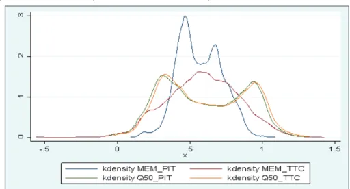
Figure 3: Kernel density estimate of the Recovery Rate forecast

Source: Authors’ calculations

The competing models are estimated on a training set of sample, out-of-sample RR forecasts are evaluated on a test sample and out-of-time. For each model, we consider the same set of explanatory variables. For each model and each sample, we compute the RR forecast. The kernel density estimates of the RR forecasts distributions displayed in Figure 3 confirm the U shape distribution for QR with two approaches PIT and TTC and for MEM with PIT.

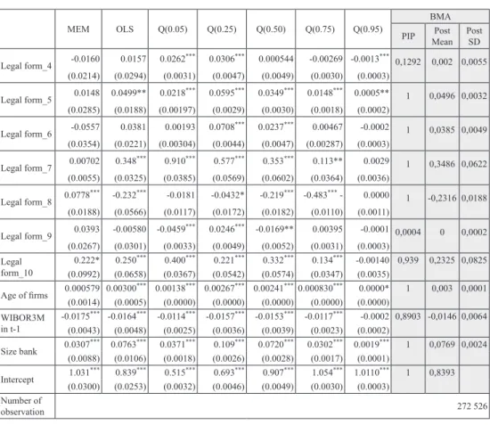
Table 3: Models of recovery rate via OLS, MEM, BMA and QR

MEM OLS Q(0.05) Q(0.25) Q(0.50) Q(0.75) Q(0.95)

BMA

PIP _MeanPost Post _SD ln_EAD -0.0078*** -0.0031* 0.0028*** 0.000192 -0.0048*** -0.0061*** -0.0004*** 1 -0,0031 0,0004 (0.0012) (0.0015) (0.0002) (0.0003) (0.0003) (0.0002) (0.0000) Collateral Indicator 0.0647 *** _0.121*** _0.0673*** _0.163*** _0.117*** _0.0491*** _0.0011*** 1 0,1213 0,0013 (0.0055) (0.0064) (0.0008) (0.0012) (0.00126) (0.0007) (0.0001) DPD_1 -0.0564*** -0.0707*** -0.335*** -0.120*** -0.0720*** -0.0361*** -0.0054*** 1 -0,0699 0,0053 (0.0118) (0.0125) (0.0032) (0.0048) (0.0051) (0.0031) (0.0003) DPD_2 -0.158*** -0.224*** -0.506*** -0.343*** -0.178*** -0.0595*** -0.0072*** 1 -0,224 0,0032 (0.0141) (0.0135) (0.0019) (0.0029) (0.0030) (0.0018) (0.0002) Time spent in default -0.00638 -0.0100* -0.0808 *** _-0.0114*** _-0.00277*** _0.00175*** _0.0000 1 -0,01 0,0008 (0.0052) (0.0041) (0.0005) (0.0007) (0.0008) (0.0004) (0.0000) DPDxTime_1 -0.00913* -0.0180*** 0.0602*** -0.0136*** -0.0184*** -0.0113*** -0.0004*** 1 -0,0178 0,0016 (0.0043) (0.00499) (0.0010) (0.0014) (0.0015) (0.0009) (0.0001) DPDxTime_2 -0.0123* -0.0295*** 0.0701*** -0.0240*** -0.0512*** -0.0399*** -0.0005*** 1 -0,0296 0,0009 (0.00500) (0.0048) (0.0006) (0.0008) (0.0008) (0.0005) (0.0001) Loan type 0.0242* 0.0355*** 0.00913*** 0.0381*** 0.0366*** 0.0122*** -0.0000 1 0,0353 0,0015 (0.0120) (0.0094) (0.00095) (0.0014) (0.0014) (0.0009) (0.0001) Guarantee Indicator 0.0282** 0.0253** 0.00366** 0.0185 *** _0.0319*** _0.0183*** _0.0008*** 1 0,0246 0,0021 (0.0106) (0.0097) (0.0013) (0.0019) (0.0020) (0.0012) (0.0001) Credit lines 0.0860*** 0.181*** 0.214*** 0.255*** 0.159*** 0.0728*** 0.0013*** 1 0,1811 0,0015 (0.0067) (0.0073) (0.0009) (0.0014) (0.0014) (0.0008) (0.0001) Bank firm relationship 0.00902 *** _{0.00393 0.00334}*** _0.0033*** _0.00328*** _0.0026*** _0.0001*** 1 0,0038 0,0004 (0.0025) (0.0024) (0.0002) (0.0003) (0.0003) (0.0002) (0.0001) Sector_2 -0.146* 0.0870** 0.0360*** 0.103*** 0.0868*** 0.0457*** 0.0013*** 1 0,0864 0,0058 (0.0627) (0.0293) (0.0036) (0.0053) (0.0056) (0.0034) (0.0003) Sector_3 0.0922*** 0.124*** 0.0303*** 0.125*** 0.135*** 0.0724*** 0.0011*** 1 0,1238 0,004 (0.0251) (0.0290) (0.0025) (0.0036) (0.0038) (0.0023) (0.0002) Sector_4 0.0334 0.000893 -0.000185 -0.000431 -0.00970*** -0.0071*** -0.0007 0,0006 0 0 (0.0273) (0.0125) (0.0012) (0.0016) (0.0017) (0.0010) (0.0001) Sector_5 -0.0227 -0.0157 -0.00450*** -0.0230*** -0.0137*** -0.0052*** -0.0003*** 1 -0,0152 0,0014 (0.0311) (0.0109) (0.0009) (0.0013) (0.0014) (0.0008) (0.00009) Sector_6 -0.0861* 0.0168 0.00180 0.00135 0.0245*** 0.0134*** 0.0001 0,9998 0,0171 0,0034 (0.0384) (0.0261) (0.0021) (0.0031) (0.0033) (0.0019) (0.0002) Sector_7 0.0210 0.117*** 0.0267*** 0.131*** 0.128*** 0.0535*** 0.0009*** 1 0,1162 0,002 (0.0268) (0.0142) (0.0013) (0.0020) (0.0021) (0.0012) (0.0001) Sector_8 0.0760* 0.0806*** 0.0127*** 0.0828*** 0.0878*** 0.0396*** 0.0005*** 1 0,0807 0,0019 (0.0322) (0.0138) (0.0013) (0.0018) (0.0019) (0.0012) (0.0001) Legal form_2 -0.00817 -0.0245* -0.0149*** -0.0189*** -0.0279*** -0.00663*** -0.0002 1 -0,0247 0,0015 (0.0101) (0.0100) (0.0009) (0.0013) (0.0014) (0.0008) (0.0001) Legal form_3 0.00219 0.0278* 0.00825*** 0.0318*** 0.0187*** 0.00915*** -0.0001 1 0,0278 0,0024 (0.0246) (0.0130) (0.0014) (0.0021) (0.0022) (0.0013) (0.0001)

MEM OLS Q(0.05) Q(0.25) Q(0.50) Q(0.75) Q(0.95) BMA PIP _MeanPost Post _SD Legal form_4 -0.0160 0.0157 0.0262*** 0.0306*** 0.000544 -0.00269 -0.0013*** 0,1292 0,002 0,0055 (0.0214) (0.0294) (0.0031) (0.0047) (0.0049) (0.0030) (0.0003) Legal form_5 0.0148 0.0499** 0.0218*** 0.0595*** 0.0349*** 0.0148*** 0.0005** 1 0,0496 0,0032 (0.0285) (0.0188) (0.00197) (0.0029) (0.0030) (0.0018) (0.0002) Legal form_6 -0.0557 0.0381 0.00193 0.0708*** 0.0237*** 0.00467 -0.0002 1 0,0385 0,0049 (0.0354) (0.0221) (0.00304) (0.0044) (0.0047) (0.00287) (0.0003) Legal form_7 0.00702 0.348*** 0.910*** 0.577*** 0.353*** 0.113** 0.0029 1 0,3486 0,0622 (0.0055) (0.0325) (0.0385) (0.0569) (0.0602) (0.0364) (0.0036) Legal form_8 0.0778*** -0.232*** -0.0181 -0.0432* -0.219*** -0.483*** - 0.0000 1 -0,2316 0,0188 (0.0188) (0.0566) (0.0117) (0.0172) (0.0182) (0.0110) (0.0011) Legal form_9 0.0393 -0.00580 -0.0459*** 0.0246*** -0.0169** 0.00395 -0.0001 0,0004 0 0,0002 (0.0267) (0.0301) (0.0033) (0.0049) (0.0052) (0.0031) (0.0003) Legal form_10 0.222* 0.250*** _0.400*** _0.221*** _0.332*** _0.134*** _{-0.00140 0,939 0,2325 0,0825} (0.0992) (0.0658) (0.0367) (0.0542) (0.0574) (0.0347) (0.0035) Age of firms 0.000579 0.00300*** 0.00138*** 0.00267*** 0.00241***0.000830*** 0.0000* 1 0,003 0,0001 (0.0014) (0.0005) (0.0000) (0.0000) (0.0000) (0.0000) (0.0000) WIBOR3M in t-1 -0.0175 *** _-0.0164*** _-0.0114*** _-0.0157*** _-0.0153*** _-0.0117*** _{-0.0002 0,8903 -0,0146 0,0064} (0.0043) (0.0048) (0.0025) (0.0036) (0.0039) (0.0023) (0.0002) Size bank 0.0307*** 0.0763*** 0.0371*** 0.109*** 0.0720*** 0.0302*** 0.0019*** 1 0,0769 0,0024 (0.0088) (0.0106) (0.0018) (0.0026) (0.0028) (0.0017) (0.0001) Intercept _(0.0300)1.031*** _(0.0253)0.839*** _(0.0032)0.515*** _(0.0046)0.693*** _(0.0049)0.907*** _(0.0030)1.054*** 1.0110_(0.0003)*** 1 0,8393 Number of observation 272 526

Note: Standard errors in parentheses; * _p<0.05, ** _p<0.01, *** _{p<0.001. Additionally, models for} all banks are estimated containing dummy variables for the different banks in addition to the variables mentioned below.

Source: Authors’ calculations

Table 4 displays’ rankings issued from four usual loss functions, namely the MSE, MAE, R2 and Kolmogorov-Smirnov (K-S) statistics. The models’ rankings that we obtain with these criteria computed with recovery Rate estimation errors. We observe that the QR model outperforms the three competing Recovery Rate models.

Table 4: Models comparison Training sample: goodness of fit

Stastistics OLS MEM QR BMA

psedo – R2 0,4330 - 0,3131 1

K – S 0,1284 0,1512 0,1074 0,1287

(p – value) (0,0001) (0,0001) (0,0001) (0,0001)

mse 0,0761 0,0947 0,0771 0,0761

mae 0,2224 0,2723 0,2181 0,2226

Validation sample: goodness of fit

Stastistics OLS MEM QR BMA

psedo – R2 0,4524 - 0,3406 1

K – S 0,1139 0,1518 0,0875 0,1011

(p – value) (0,0001) (0,0001) (0,0001) (0,0001)

mse 0,0722 0,0942 0,0720 0,0755

mae 0,2168 0,2693 0,2078 0,2134

Out-of-sample: goodness of fit

Stastistics OLS MEM QR BMA

psedo – R2 0,4352 - 0,3164 1

K – S 0,1272 0,1502 0,1063 0,1267

(p – value) (0,0001) (0,0001) (0,0001) (0,0001)

mse 0,0755 0,0933 0,0765 0,0745

mae 0,2213 0,2702 0,2170 0,2207

Source: Authors’ calculations

5. Results and discussion

Based on the estimation of the Recovery Rate model, Loss Given Default was obtained. The stability of the model was checked using three sets: training sample, validation data and testing sample (out-of-time). On the basis of the measurements used in the validation process, the model was not overestimated. Based on the estimated recovery rates, in practice, provisions are estimated for a given period. In order to calculate provisions for a given period, individual risk parameters for the loan portfolio comprising the Expected Credit Loss (ECL) should be calculated: the probability of default (PD), exposure at default (EAD) and loss given default (LGD). The latest data in the sample is data for 2018. For this reason, provisions for

default and non-default observations for expected credit losses have been calculated for this year.

For Poland non-financial corporations, Credit Assessment System (see: Nehrebecka, 2016) can estimate the risk of default during the coming year (parameter PD). In the case of LGD, the values predicted by the model built were used. In order to calculate the reserves, simplified formulas were used:

Bank reserves2018_stage1 = PD * EAD * LGDnon-default (1)

where: LGDnon-default = 1 – RRnon-default

Bank reserves2018_stage3 = PD * EAD * LGDdefault (2)

where: LGDdefault = 1 – RRdefault

Based on the above analysis, it was calculated that for loans in default from 2018, reserves amounting to PLN 4 158 million should be assumed, which constitutes 31% of the loan portfolio in default (Table 5). For healthy loans appearing in 2018, a reserves for expected credit losses in the amount of PLN 2 125 million should be made, which is 1% of the total liabilities of a healthy portfolio. Based on the annual report of the Polish Financial Supervision Authority on the condition of banks, the amount of reserves in the entire banking sector in 2017 amounted to PLN 9 505 million for 616 of the analyzed entities conducting banking activities (including 35 commercial banks).

Table 5: Summary of the value of calculated provisions for 2018 for liabilities in default and non-default

Amount Mean _PD Mean _LGD Portfolio(in mln PLN) Bank reserves (in PLN) Bank reserves (in %)

Portfolio Credit Default 528 - 31% 13 414 4 158 31%

Portfolio Credit Non-Default 14 023 5% 20% 212 557 2 125 1%

Source: Authors’ calculations

Taking these elements into account, it can be stated that the estimated model gives good results on which to base the initial analysis in terms of the reserves created.

6. Conclusions

The purpose of this research is to model the loss due to the LGD’s default. LGD is one of the key modelling components of the credit risk capital requirements. There is no particular guideline has been processed concerning how LGD models should

be compared, selected, and evaluated. Recent LGD models mainly focus on mean predictions. We show that in order to estimate the risk parameter of LGD, a number of requirements imposed by the regulator should be met in an appropriate manner. The main aspects are the right approach to the default definition – consistent within all credit risk parameters, creating a reliable reference data set, based on which the LGD is estimated, considering all historical defaults in modeling and selecting the appropriate modeling method. It is necessary to verify and validate the methods, which are estimated losses due to defaults and to correct any discrepancies. Validation should pay attention to compliance with regulatory requirements as well as the correctness of the estimated parameters and the predictive power of models. Correct estimation of the LGD parameter affects the maintenance of adequate capital for expected credit losses, which is a key element of the bank operation. The recovery rate defined as the percentage of the recovered exposure in the case of default is usually bimodal, which means that most exposures are recovered almost one hundred percent or are not recovered at all.

Based on the survey review, the following conclusions can be drawn in terms of factors affecting the recovery rate. The most frequent, significantly affecting the recovery rate were the loan collateral, positively affecting recovery rate, loan size, usually negative impact on the explained variable, the classification of the liability with positive impact on the Recovery Rate and the division into business sectors (the lowest rate of recovery was usually the trade sector).

The paper also describes the current requirements for a new approach to calculating reserves for expected credit losses, and thus a new approach to the LGD risk parameter. For loans in default from 2018, reserves amounting to PLN 4 158 million should be assumed, which constitutes 31% of the loan portfolio in default.

For healthy loans appearing in 2018, a reserves for expected credit losses in the amount of PLN 2 125 million should be made, which is 1% of the total liabilities of a healthy portfolio.

The methods used are very sensitive to the size of random error from the fact that the adjustment of the LGD parameter value has a strong bimodal distribution. The quantile regression method proved to be a good tool for predicting recovery rates. Its stability was checked using three sets – training, validation and test data with data outside of the training sample. All models obtained similar RMSE measures, indicating the lack of overestimation of the model. It is also possible to estimate the cost of recovery of deferred loans based on the analyzed database. Taking these elements into account, it can be stated that the estimated model gives good results on which to base the initial analysis in terms of the reserves created.

The results obtained indicate the importance of research results for financial institutions for which the model proved to be a more effective method of estimating LGD under the internal rating based on the Basel agreement. The results obtained

may be economically significant for regulators, because problems that arise during the analysis may lead to an underestimation of the loss level.

References

Altman, E., Gande, A., Saunders, A. (2010) “Bank Debt Versus Bond Debt: Evidence from Secondary Market Prices”, Journal of Money, Credit and

Banking, Vol. 42, No. 4, pp. 755–767, doi: 10.1111/j.1538-4616.2010.00306.x. Altman, E.I., Kalotay, E.A. (2014) “Ultimate recovery mixtures”, Journal of Banking

& Finance, Vol. 40, No. 1, pp. 116–129, doi: 10.1016/j.jbankfin.2013.11.021. Archaya, V. V., Bharatha, S. T., Srinivasana, A. (2007) “Does Industry-Wide

Distress Affect Defaulted Firms? Evidence From Creditor Recoveries”, Journal

of Financial Economics, Vol. 85, No. 3, pp. 787–821, doi: 10.1016/j.jfineco. 2006.05.011.

Arner, R., Cantor, R., Emery, K. (2004) “Recovery Rates on North American Syndicated Bank Loans, 1989-2003”, Moody’s Special Comments. Available at <http://www. moodyskmv.com>, [Accessed: January 06, 2019].

Asarnov, E., Edwards, D. (1995) “Measuring Loss on Defaulted Bank Loans: A 24 year study”, Journal of Commercial Lending, Vol. 77, No. 7, pp. 11–23.

Basel Committee on Banking Supervision (2005) International Convergence of Capital Measurement and Capital Standards: A Revised Framework, Basel: Bank for International Settlements.

Basel Committee on Banking Supervision (2005) “Studies on the Validation of Internal Rating Systems”, Working Paper (Internet], Vol. 14. Available at <http://www.forecastingsolutions.com/downloads/Basel_Validations.pdf>, [Accessed: January 06, 2019].

Bastos, J. A. (2010) “Forecasting bank loans loss-given-default”, Journal of Banking

& Finance, Vol. 34, No. 10, pp. 2510-2517, doi: 10.1016/j.jbankfin.2010.04.01. Bastos, J. A. (2010) “Predicting bank loan recovery rates with neural networks”,

Center for Applied Mathematics and Economics Lisbon (Internet]. Available at <https://core.ac.uk/download/pdf/6291858.pdf>, [Accessed: January 06, 2019]. Belyaev, K., Belyaeva, A., Konečný, T., Seidler, J., Vojtek, M. (2012)

“Macroeconomic Factors as Drivers of LGD Prediction: Empirical Evidence from the Czech Republic”, CNB Working Paper (Internet], Vol. 12. Available at <https://www.cnb.cz/miranda2/export/sites/www.cnb.cz/en/research/research_ publications/cnb_wp/download/cnbwp_2012_12.pdf>, [Accessed: January 06, 2019].

Board of Governors of the Federal Reserve System (2006) “Risk-based Capital Standards: Advanced Capital Adequacy Framework and Market Risk” Fed.