Durham Research Online
Deposited in DRO:28 November 2014
Version of attached le: Accepted Version
Peer-review status of attached le: Peer-reviewed
Citation for published item:
Coolen, F.P.A. and Coolen-Maturi, T. (2015) 'Predictive inference for system reliability after common-cause component failures.', Reliability engineering system safety., 135 . pp. 27-33.
Further information on publisher's website:
http://dx.doi.org/10.1016/j.ress.2014.11.005
Publisher's copyright statement:
NOTICE: this is the author's version of a work that was accepted for publication in Reliability Engineering System Safety. Changes resulting from the publishing process, such as peer review, editing, corrections, structural formatting, and other quality control mechanisms may not be reected in this document. Changes may have been made to this work since it was submitted for publication. A denitive version was subsequently published in Reliability Engineering System Safety, 135, March 2015, 10.1016/j.ress.2014.11.005.
Additional information:
Use policy
The full-text may be used and/or reproduced, and given to third parties in any format or medium, without prior permission or charge, for personal research or study, educational, or not-for-prot purposes provided that:
• a full bibliographic reference is made to the original source
• alinkis made to the metadata record in DRO
• the full-text is not changed in any way
The full-text must not be sold in any format or medium without the formal permission of the copyright holders. Please consult thefull DRO policyfor further details.
Predictive inference for system reliability after
common-cause component failures
Frank P.A. Coolen1a, Tahani Coolen-Maturi2
1Department of Mathematical Sciences, Durham University, UK 2Durham University Business School, Durham University, UK
Abstract
This paper presents nonparametric predictive inference for system reliability following common-cause failures of components. It is assumed that a single failure event may lead to simultaneous failure of multiple components. Data consist of frequencies of such events involving particular numbers of compo-nents. These data are used to predict the number of components that will fail at the next failure event. The effect of failure of one or more components on the system reliability is taken into account through the system’s survival signature. The predictive performance of the approach, in which uncertainty is quantified using lower and upper probabilities, is analysed with the use of ROC curves. While this approach is presented for a basic scenario of a system consisting of only a single type of components and without consider-ation of failure behaviour over time, it provides many opportunities for more general modelling and inference, these are briefly discussed together with the related research challenges.
Keywords: Common-cause failures, lower and upper probabilities,
nonparametric predictive inference, ROC curves, survival signature, system reliability
1. INTRODUCTION
A major consideration for reliability of systems is the possible occurrence of common-cause failures, where multiple components fail simultaneously due to the same underlying cause. This paper considers the reliability of a system
following a future failure event, with possible common-cause failures of mul-tiple components. In particular, the aim is to develop predictive inference for the reliability of a system with multiple components based on previous failure event data for this system, or for other systems that are fully exchangeable with this system. These data are assumed to consist of the numbers of failing components in past failure events, in each of which at least one component failed. These failure events did not necessarily involve failure of the whole system, but each event involves failure of one or more components. Aspects of ageing are not taken into account, nor any other aspects that are explicitly related to time, usage or other processes. Such aspects are likely to be im-portant in some practical applications, developing methodology to deal with these provides interesting research challenges.
Common-cause failures are important in many applications, as systems with built in redundancy are at increased risk if multiple components may fail simultaneously. Basic concepts of modelling common-cause failures are reviewed by Rasmuson and Kelly [1] and by Mosleh et al [2]. The alpha-factor model, proposed by Mosleh et al [3] is commonly used, and enables straightforward analysis in the framework of Bayesian statistics due to the availability of conjugate prior distributions [4]. A robust Bayesian approach to this model has recently been proposed by Troffaes et al [5], using a set of conjugate priors instead of a single prior distribution, following a standard approach for generalized Bayesian methods in theory of imprecise probabil-ities [6]. In this paper an alternative statistical method within the theory of imprecise probability is used, namely nonparametric predictive inference (NPI) [7]. For the problem considered here, it makes little difference which specific method for statistical inference is used to predict the number of com-ponents failing simultaneously at the next common-cause failure event. Due to its explicitly predictive nature it is attractive to use the NPI approach. The main contribution of the paper is the link from inference on this number of failing components to lower and upper probabilities for the event that the system will still function after the next common-cause failure event. This link is quite straightforward, as shown in this paper, with the use of the system survival signature [8], a recently introduced concept which is closely related to the popular system signature [9] but, in contrast to the latter, is also conceptually straightforward for systems with multiple types of com-ponents. The question of the system’s reliability following a common-cause failure event is of practical interest, as following such an event one may have more time to consider appropriate maintenance or replacement actions if the
system is still functioning than in case the system has failed. Such further actions are not addressed in this paper, but combined with aspects of failure processes they provide interesting topics for future research.
As mentioned, the main contribution of this paper is to model the link be-tween failure of components and failure of the system, or indeed functioning of the system, for the common-cause failure scenario, through the recently in-troduced concept of survival signatures [8]. For a system withmcomponents, the state vector x= (x1, x2, . . . , xm)∈ {0,1}m is defined such that xi = 1 if
the ith component functions and xi = 0 if not, using an arbitrary but fixed
labelling of the components. The structure function φ : {0,1}m → {0,1},
defined for all possible x, takes the value 1 if the system functions and 0 if the system does not function for the state vector x. The structure function can be generalized by defining it as the probability that the system functions for the state vector x, which might be relevant if one is not certain about its functioning [10], this is not used in this paper but provides interesting challenges for research and opportunities for applications.
In this paper, attention is restricted to coherent systems, which means that φ(x) is not decreasing in any of the components of x, so system func-tioning can never be improved by worse performance of one or more of its components. It is further assumed that φ(0) = 0 andφ(1) = 1, so the system fails if all its components fail and it functions if all its components function. These assumptions could easily be relaxed but they simplify presentation in this paper and are reasonable for most systems of practical interest. More importantly, attention is restricted in this paper to systems consisting of ex-changeable components, which could be called components of a single type. Most practical systems, in particular also networks, consist of components of multiple types. This restriction is merely for sake of simplicity of presenta-tion, the method introduced here can quite straightforwardly be generalized to systems with multiple types of components.
The survival signature for a system withmexchangeable components, de-noted by Φ(l), for l = 1, . . . , m, is the probability that the system functions given that precisely l of its components function [8]. For coherent systems, Φ(l) is an increasing function of l, and the second assumption above leads to Φ(0) = 0 and Φ(m) = 1. There are ml state vectors x with precisely l
components xi = 1, so with
Pm
i=1xi =l; let Sl denote the set of these state
vectors. Due to the exchangeability assumption for the m components, or more precisely the assumed exchangeability of the random quantities repre-senting functioning of the m components, all these state vectors are equally
likely to occur, hence Φ(l) = m l −1 X x∈Sl φ(x) (1)
Coolen and Coolen-Maturi [8] called Φ(l) the survival signature because, by its definition, it is closely related to survival of the system, and it is close in nature to the system signature [9]. The survival signature can straight-forwardly be generalized to systems with multiple types of components, in contrast to the system signatures for which this is practically impossible [8]. This paper is organised as follows. Section 2 presents the use of non-parametric predictive inference to predict the number of failing components at a future common-cause failure event. In Section 3 these inferences are combined with the survival signature to lead to lower and upper probabil-ities for the event that the system will still function after the next failure event. As with any newly proposed procedure, it is important to evaluate the performance of the presented method, this is non-trivial for methods us-ing lower and upper probabilities. In Section 4 a novel way to evaluate the performance of such an imprecise probability method is introduced, which is fully in line with the predictive nature of the inferences and makes use of ROC curves. Section 5 concludes the paper with a discussion of the method and related research challenges.
2. PREDICTING THE NUMBER OF FAILING COMPONENTS
For a system withmexchangeable components, which are assumed through-out this paper to all function before the failure event of interest, a common-cause failure event can lead to simultaneous failure of any number f ∈ {1, . . . , m} of components. The alpha-factor model [2, 3] introduces param-eters αj, for j = 1, . . . , m, representing the probability that precisely j of
the m components in the system fail simultaneously, given that a failure event occurs, hence Pm
j=1αj = 1. It is possible to select values αj based
on background knowledge of the system, but in this paper we aim at learn-ing about these probabilities from available failure data whilst attemptlearn-ing to add only rather minimal further assumptions. Recently, two Bayesian solu-tions to the same problem have been presented, one using a non-informative Dirichlet prior distribution [4] and the other using the imprecise Dirichlet model (IDM) [5]. Both of these let the numbers 1 to m of possible simulta-neous failures be represented by m categories, with an assumed multinomial
distribution for the numbers of observations in these categories. This is a standard statistical approach, with the IDM the most widely applied impre-cise probability model in statistics [6, 11] with also interesting applications in reliability, see for example [12, 13]. There are, however, two issues with this model. Even while the (set of) prior distribution(s) is chosen in order to have little influence on the inferences, they do affect these noticeably in case interest is in categories which have rarely or even never been observed. Furthermore, any ordering of the categories is not taken into account. The latter aspect is particularly relevant if one is interested in events involving unions of categories, for example that the number of simultaneously failing components is at least two.
This paper presents a nonparametric predictive inference (NPI) alterna-tive to the combination of the alpha-factor model with (imprecise) Dirichlet prior(s), also using lower and upper probabilities to quantify uncertainty. NPI for multinomial data has been presented as an alternative to the IDM [14], while NPI for real-valued data, including right-censored observations, has also been applied successfully [15, 16]. However, in this paper attention is restricted to NPI for ordinal data [17] as this explicitly takes the natural ordering of the m categories, namely the numbers 1, . . . , m, into account. Assume that data are available on n previous common-cause failure events, which are assumed to be exchangeable with the next event, implying that they also all involved m components, and all components, in the observed systems and for the prediction, are exchangeable. Let nj ≥ 0 denote the
number of the observed common-cause events in which precisely j compo-nents failed simultaneously, so Pm
j=1nj = n. It is important to emphasize that no information or assumption is used about which specific components failed, just the numbers of components failing at the failure events are of interest for the inferences considered in this paper.
It is important to comment briefly on the assumption of exchangeability of all components, both in the observed systems and for prediction. For simplicity, one can consider this assumption as being in line with assuming all components have the same (unknown) probability of failure in case of a common-cause failure event. Hence, one could not, for example, apply the method presented in this paper in a scenario where components that have been in a system for a longer time undergo some wear, in the sense of their probability of failure increasing. If one would deem new components in a system, which replace failed components, to have a lower probability of failure upon a future common-cause failure event than other components in
the system, then one would need to distinguish the components into different types. This can also be modelled through the general concept of the survival signature, but for simplicity of presentation this paper restricts attention to components of a single type. There are, however, scenarios where it seems quite reasonable to assume exchangeability of the components in case of a common-cause failure event, for example if the cause of the failures is due to shocks and the components’ capacity to deal with such shocks is independent of their age.
NPI for ordinal data [17] provides lower and upper probabilities for events involving the number Yn+1 of failing components at the next, son+ 1-st, fail-ure event. These NPI lower and upper probabilities are not available in ana-lytic form for all possible events Yn+1 ∈C with C any subset of {1, . . . , m}, generally they are calculated via counting of orderings in an assumed underly-ing latent variable representation, with a real-valued latent variable assumed to fall into the different categories, ordered on the real-line, determining the observation category. Such an underlying model assumption is rather com-mon in statistics as it leads to quite simple models, but in addition it may be quite realistic in common-cause failure scenarios, for example one might consider there to be an underlying variable corresponding to strength of the cause of the failure event (e.g. strength of wind or earth quake) that would not be directly observable but could play a crucial role in determining the number of simultaneously failing components. There are some special events for which closed-form expressions are available [17] and these include the events required for the theory presented in Section 3 in this paper. This spe-cial case involves events of the form Yn+1 ∈ {s, . . . , t}, with 1 ≤s ≤t ≤ m, so the event that the number of components which fail simultaneously at the next failure event is any value froms tot. This includes events involving just a single number (s =t), events that the number of failing components is at least s (with t=m), and at most t (with s = 1). The event with s= 1 and
t =m is trivially true, so both the NPI lower and upper probabilities for this event are equal to 1 and this event is excluded from further consideration. Letns,t=
Pt
upper probabilities for such events are [17] P(Yn+1 ∈ {s, . . . , t}) = (ns,t−1)+ n+ 1 if 1< s≤t < m ns,t n+ 1 if s= 1 ort =m (2) P(Yn+1 ∈ {s, . . . , t}) = ns,t+ 1 n+ 1 for 1≤s≤t≤m (3)
The method presented in this paper uses the lower and upper cumulative distribution functions (CDF), which immediately follow from (2) and (3), with for j ∈ {1, . . . , m−1} F(j) = P(Yn+1 ≤j) = n1,j n+ 1 (4) F(j) = P(Yn+1 ≤j) = n1,j+ 1 n+ 1 (5)
andF(m) =F(m) = 1. Note thatYn+1 cannot be equal to 0, as it is assumed that at least one component fails at a failure event, hence F(0) = F(0) = 0. It is important to emphasize that these NPI lower and upper probabilities are frequentist statistics inferences [6, 7], and can be interpreted as bounds for a confidence level in the occurrence of the stated event of interest, based on the available data. The confidence interpretation results from the exchange-ability assumption and can be interpreted as a long-run frequency where, for varying data sets but with exchangeability of observed data and the future observation for each run, the proportion of times that the event will indeed occur will be between the NPI lower and upper probabilities.
3. SYSTEM RELIABILITY AFTER FAILURE EVENT
The survival signature Φ(l) for a system consisting of m exchangeable components represents the probability that the system functions if precisely
l of its components function. So the functioning of the system after the next common-cause failure event can be predicted by combining the survival signature and NPI for ordinal data, as presented in Section 2. The NPI lower probability for the event S that the system still functions after the
next common-cause failure event is P(S) = m X j=1 Φ(m−j) [F(j)−F(j−1)] (6) = m−1 X j=1 nj n+ 1Φ(m−j) (7) and the corresponding NPI upper probability is
P(S) = m X j=1 Φ(m−j)F(j)−F(j −1) (8) = n1+ 1 n+ 1Φ(m−1) + m−1 X j=2 nj n+ 1Φ(m−j) (9) Here the logical assumption Φ(0) = 0 has been used, so the system does not function if none of its components function. Furthermore, the assumption that the system is coherent has been used, hence the system survival signature Φ(l) is non-decreasing in l. These results imply that
P(S) = P(S) + Φ(m−1)
n+ 1 (10)
These NPI lower and upper probabilities are derived by minimising and maximising, respectively, the probability for event S corresponding to ev-ery possible precise probability distribution within the bounds specified by the NPI results presented in Section 2. For non-coherent systems the ap-proach can also be used, but the optimisation results are not available in general forms. For a series system, Φ(m) = 1 and Φ(l) = 0 for all l < m, so P(S) = P(S) = 0, which is trivial as a series system cannot function if at least one of its components has failed. For a parallel system, Φ(l) = 1 for all l ≥ 1 so P(S) = n1,m−1 n+1 = n−nm n+1 and P(S) = n1,m−1+1 n+1 = n−nm+1 n+1 . For a
k-out-of-m system with k∈ {2, . . . , m−1}, which functions if and only if at least k of its m components function, Φ(l) = 1 for l ≥ k and Φ(l) = 0 for
l < k, hence P(S) = n1,m−k
n+1 and P(S) =
n1,m−k+1
n+1 .
From Equation (10) the imprecision ∆(S) for eventS, which is the differ-ence between the corresponding NPI upper and lower probabilities for this event, follows immediately,
∆(S) = P(S)−P(S) = Φ(m−1)
2 1
5 4 3
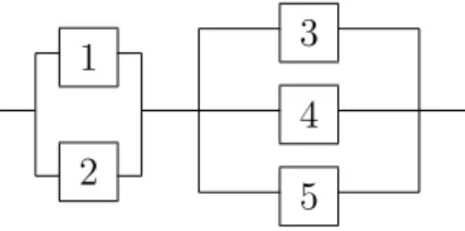
Figure 1: System for Example 1
This imprecision is obviously decreasing as function ofn, which is fully in line with intuition. Furthermore, straightforward analysis can be used to derive relations between the NPI lower (or upper) probabilities for the eventSfor a specific system based on different data sets in which all categories have been observed in the same proportion. Consider a data set A with in total na
observed failure events, of which naj involved precisely j failing components, and data set B with in total nb = wna observed failure events, of which
nb
j = wnaj involved precisely j failing components, and w >1 such that the
resulting nbj are all integers. While there is not much insight to be gained from such relations, it follows easily that, for all such w >1, the NPI lower and upper probabilities are logically nested, that is
Pa(S)≤Pb(S)≤Pˆ(S)≤Pb(S)≤Pa(S) (12)
where ˆP(S) =Pm−1
j=1
nj
nΦ(m−j), the empirical estimator for the probability
that the system functions, as based on the empirical proportions nj
n of the
observations for each number of simultaneously failing components. The NPI approach always provides lower and upper probabilities that bound the corresponding empirical estimator in this logical way [7, 18]. All inequalities in (12) tend to be strict except in some trivial cases with either values equal to 0 or 1.
Example 1.
The system in Figure 1 has the survival signature with the following val-ues: Φ(1) = 0, Φ(2) = 0.6, Φ(3) = 0.9 and Φ(4) = 1, in addition to the trivial values Φ(0) = 0 and Φ(5) = 1. Suppose that n = 10 failure events for com-ponents of such a system have been observed, with n1 = 4 events involving a
7 6 5 4 3 2 1
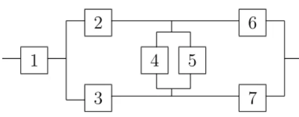
Figure 2: System for Example 2
single failing component,n2 = 3 events involving simultaneous failure of two components, and n3 = 2, n4 = 0 and n5 = 1 the number of events involv-ing the simultaneous failure of three, four and five components, respectively. Interest is in the event S that the system, with all its components currently functioning, will still function after the next failure event, which is assumed to be exchangeable with these 10 previous events with regard to the number of simultaneously failing components. The NPI lower probability for this event, given by Equation (7), is P(S) = 0.718 and the corresponding NPI upper probability, given by Equation (9), is P(S) = 0.809. The imprecision in this case is ∆(S) = Φ(4)11 = 0.091.
As a second data set for the same system consider n = 40 failure events with n1 = 25, n2 = 10, n3 = 4, n4 = 1 and n5 = 0. This leads to NPI lower probability P(S) = 0.888 and P(S) = 0.912. The imprecision in this case is ∆(S) = Φ(4)41 = 0.024.
Example 2.
The system in Figure 2 was used by Al-nefaiee and Coolen [19] to illus-trate specific aspects of nonparametric predictive inference for system failure time using the system signature. The system signature and system survival signature are directly related for systems with a single type of components, as discussed by Coolen and Coolen-Maturi [8]. The survival signature for this system is given by Φ(1) = Φ(2) = 0, Φ(3) = 0.057, Φ(4) = 0.343, Φ(5) = 0.619, Φ(6) = 0.857 and the trivial values Φ(0) = 0 and Φ(7) = 1.
Suppose first that available data consist of n = 100 observed failure events, with n1 = 70, n2 = 20, n3 = 10 and nj = 0 for j ∈ {4, . . . ,7}.
0.7591 for system functioning after the next failure event, with imprecision ∆(S) = P(S)−P(S) = Φ(6)101 = 0.0085. If there are only n = 10 observa-tions, with numbers of failing components occurring in the same ratios, so
n1 = 7, n2 = 2, n3 = 1 andnj = 0 forj ∈ {4, . . . ,7}, then the corresponding
NPI lower and upper probabilities are P(S) = 0.6892 and P(S) = 0.7671, with imprecision ∆(S) = Φ(6)11 = 0.0779. Together with ˆP(S) = 0.7581 these values illustrate the inequalities (12).
Consider further the same data with n = 100 except now with n3 = 9 and n7 = 1, so for one observed failure event actually all 7 components failed instead of just three. This leads to P(S) = 0.7472 and P(S) = 0.7557, so both slightly smaller than for the earlier case with the nearly identical 100 observations, while the imprecision remains equal to ∆(S) = 0.0085.
4. PERFORMANCE EVALUATION
The method for prediction of system functioning after a future common-cause failure event, as presented in Section 3, is quite straightforward and leads, for each individual application, to lower and upper probabilities for the event that the system will still function after such an event. Due to the use of NPI, these lower and upper probabilities have powerful properties in the frequentist statistics framework [7], and the imprecision, so the difference between the corresponding upper and lower probabilities, reflects the amount of information in the available data. It is important to investigate the be-haviour of this method further, in particular to get insight into the quality of the predictions. Due to the use of lower and upper probabilities this is not straightforward, because the additional dimension of uncertainty, reflecting the indeterminacy through imprecision, may not have a clear benefit per se. Indeed, the imprecision is a consequence of limited information from data and limited assumptions. Zaffalon et al [20] have proposed a method to measure the quality of an imprecise prediction by a single number. Their metric consists of an objective component and an aspect related to the de-cision maker’s risk aversion to variability of predictions. Such an approach has advantages, as in contrast to intervals, single numbers can be uniquely ordered, which is helpful to compare different methods. However, an alter-native method is proposed here to illustrate and investigate the performance of the presented predictive method. This novel method for performance eval-uation does not rely on subjective input and reflects imprecision, which is
important, for example, to study the effect of the number of available data on the inferences.
This new method for investigating the performance of imprecise predic-tive inferences is presented and applied to investigate how the inferential method presented in Section 3 is influenced by the number of available data. The new method uses the theory of Receiver Operating Characteristic (ROC) curves, a well established method for comparison of the performance of di-agnostic methods [21, 22]. While main developments and applications of ROC methods have mostly been reported in medical statistics, they have been increasingly applied in recent years, including to reliability problems. For example, they have been used for the comparison of different statistical models for failures in water supply networks [23] and steel coil manufactur-ing [24]. Only basic nonparametric methods for ROC analysis are used in this paper, with necessary adaptation to deal with imprecise probabilities as inputs. It is, however, worth mentioning that NPI provides an interesting alternative to the established ROC methods, again with a fully predictive nature [25], its application to scenarios as considered in this paper is left as a topic for future research.
The method presented in Section 3 has as input the numbers nj, for
j = 1, . . . , m, of events in which j components failed simultaneously, with data of in total n = Pm
j=1nj events. The output of the method consists of the corresponding NPI lower and upper probabilities, P(S) and P(S), for the event S that the system still functions after the next failure event. At the moment these lower and upper probabilities are calculated, the actual future functioning status of the system will of course be unknown, hence these lower and upper probabilities can be regarded as a diagnostic tool, with higher values more indicative of system functioning. Insight into the performance of this method can be gained through simulation studies, which are described next. It is important here to simulate in such a manner that the quality of the prediction can be investigated. This can be achieved by simulating several cases involving different mixtures of distributions, and then to see if the method picks up the difference well in its predictions. Furthermore, the simulations will illustrate the effect on the inferences of the amount of data available, where typically imprecision should tend to decrease with increasing numbers of available data.
The simulation study is performed as follows, describing one run in detail. Two probability distributions are assumed over the integers {1,2, . . . , m},
from eachn+1 values are sampled with replacement. Of thesen+1 values for each distribution, one is drawn by simple random sampling, this will serve as a future observation and be denoted bynf. The remainingn values sampled
from each distribution serve as data, with nj the number of times the value
j is included in this simulated data set. Interestingly, it is not important how these n+ 1 values are simulated as the NPI approach only requires the future observation of interest to be exchangeable with the observed data, which is ensured by the random selection of one of these n+ 1 values to serve as the future observation. The NPI lower and upper probabilities, P(S) and
P(S), are calculated on the basis of this simulated data set{n1, . . . , nm}. The
simulated future observationnf functions as the number out ofmcomponents
failing at the next failure event, and is used to simulate an actual future observation of the functioning status of the system by drawing a value for a Bernoulli distributed random quantity Sf which takes the valueSf = 1 with
probability Φ(m−nf) and Sf = 0 else. Hence, Sf simulates the status of
the system after the next failure event, with Sf = 1 indicating functioning
and Sf = 0 failure of the system.
The resulting output from one simulation run is a triple (P(S), P(S), Sf)
for each of the two distributions used for the simulation. The full simulation study consists of a predetermined numberK of such independent runs, lead-ing to 2K such triples. It is important here that two (or more) probability distributions have been used for the simulations, if only a single distribution were used all values Sf would have been exchangeable and it would not
al-low investigation of success of the method as there would not be any reason why higher values of P and P would tend to correspond to value Sf = 1
than for lower values of P and P. Informally, the performance of the pre-dictive method is good if values Sf = 1 occur mostly in triples with higher
values of P(S) and P(S) while Sf = 0 occurs mostly in triples with lower
values of P(S) andP(S). Hence, these lower and upper probabilities can be considered as diagnostic tools to indicate the future system status, enabling the method’s performance to be evaluated using ROC analysis based on the output of these simulations. In particular, the area under the ROC curve (AUC) is an established tool to measure the diagnostic quality of a classi-fication method, where AUC of about 0.5 indicates that the method does not perform better than random allocation while AUC close to 1 indicates excellent performance.
In order to investigate the method’s performance, the data resulting from the K simulation runs, so in total 2K triples (P(S), P(S), Sf) as in each
run two probability distributions were used, are divided into two groups, depending on the value of Sf. So Sf = 1 for one group of simulation runs
with the system functioning after the next failure event, let K1 denote the number of simulation runs for which the output is in this group. Similarly,
Sf = 0 for the group of simulation runs with the system failing at the next
failure event, the number of simulation runs in this group is denoted by
K0, of course K0 +K1 = 2K. Application of ROC analysis to indicate the performance of this method would now be relatively straightforward, e.g. using standard nonparametric methods for such an analysis in order not to make further modelling assumptions, apart from the fact that the indicators consist of intervals [P(S), P(S)] for each run, while normally for ROC analysis the information on which to base the diagnosis is assumed to be a single value. To deal with this, optimal bounds for the ROC analysis for all possible combinations of probabilities within the intervals [P(S), P(S)] can be derived, as described next. These bounds reflect the imprecision in the NPI method.
Some further notation is introduced for this ROC analysis. For simula-tion run j ∈ {1, . . . , K1}with Sf = 1, the NPI lower and upper probabilities
for the event that the system will function at the next observation are de-noted by P1j(S) and Pj1(S), respectively. For simulation run l ∈ {1, . . . , K0} with Sf = 0, the corresponding notation is P0l(S) and P
0
l(S). For any set
of probabilities p1 j ∈[P 1 j(S), P 1 j(S)], j = 1, . . . , K1, and p0l ∈[P 0 l(S), P 0 l(S)],
l = 1, . . . , K0, there is a single corresponding nonparametric estimate of the ROC curve, say ROC(p1, p0) with p1 = (p11, . . . , pK11) and p0 = (p01, . . . , p0K0). It is easy to see that these ROC curve estimates depend monotonically on
p1 and p0. If an element of p1 is increased then the ROC curve can only change by moving upwards, with the area under the ROC curve (denoted by AUC) increasing. Similarly, if an element of p0 is increased then the ROC curve can only change by moving downwards, with the AUC decreas-ing. This implies that the set of all ROC(p1, p0) with p1
j ∈ [P1j(S), P 1 j(S)], j = 1, . . . , K1, and p0l ∈ [P 0 l(S), P 0 l(S)], l = 1, . . . , K0, is bounded from below by ROC = ROC(P1(S), P0(S)), with P1(S) = (P11(S), . . . , P1K1(S)) and P0(S) = (P01(S), . . . , P0K
0(S)), and this set is bounded from above
by ROC = ROC(P1(S), P0(S)), with P1(S) = (P11(S), . . . , P1K1(S)) and
P0(S) = (P01(S), . . . , P0K
0(S)). Of course, these bounds are optimal because
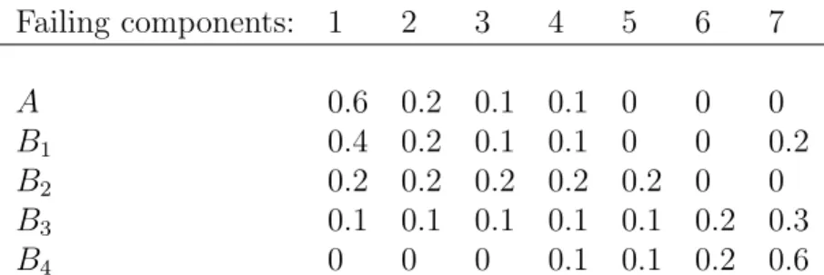
proba-Failing components: 1 2 3 4 5 6 7 A 0.6 0.2 0.1 0.1 0 0 0 B1 0.4 0.2 0.1 0.1 0 0 0.2 B2 0.2 0.2 0.2 0.2 0.2 0 0 B3 0.1 0.1 0.1 0.1 0.1 0.2 0.3 B4 0 0 0 0.1 0.1 0.2 0.6 Table 1: Probability distributions used in 4 cases for simulation
Case 1 2 3 4
n = 10 (0.3653,0.7291) (0.5225,0.7755) (0.6470,0.8459) (0.8041,0.9416)
n = 100 (0.5361,0.6121) (0.6274,0.6987) (0.7228,0.7893) (0.8528,0.9041)
n = 500 (0.5622,0.5969) (0.6491,0.6827) (0.7277,0.7587) (0.8592,0.8832) Table 2: Results (AU C, AU C) of simulation study
bilities as indicated. Optimal bounds for the AUC values for all considered ROC curves follow immediately, with the lower bound AUC the area under ROC and the upper bound AUC the area under ROC.
The method is now implemented for the system in Example 2 in Section 3. Four cases have been investigated, with two probability distributions over the integers {1, . . . ,7} used in each case. These cases are specified in Table 1. One distribution was kept constant, it is indicated as distribution A. The second distribution used differs per case, and is indicated by Bi for Case
i∈ {1,2,3,4}.
Note that the probability distributions B3 and particularly B4, used in Cases 3 and 4, are substantially different from probability distribution A. Therefore, in Cases 3 and 4 the method should be able to perform well in prediction, as higher values of P(S) and P will be more likely to result from the simulations using probability distribution B3 orB4 than those using A, and hence the corresponding predicted status of the system will also more likely be a failure. Table 2 presents the values AU C and AU C for this investigation, all based on K = 1,000 simulation runs (hence with 2,000 simulated triples in each full simulation), and with different sizes n of the simulated data sets.
with expectations. The quality of prediction increases if the two probability distributions included in one simulation case differ more substantially, and the imprecision AU C−AU C decreases for larger values of n. For n = 10, the value of AU C for Case 1 is less than 0.5, which might be interpreted as indicating that a classification performance better than random allocation is not guaranteed in this case, but it is certainly possible given that the corresponding AU C is greater than 0.5. This is actually not surprising as the two distributions used in Case 1 do not differ very much and the number of observations used in each simulation is small. These simulations were also carried out with larger values of K, but the results were close to those reported in Table 2.
This performance evaluation method has been presented here in detail as it appears not to have been reported in the literature before, and it has the clear advantage of reflecting, through the imprecision, the influence of the amount of available data on the performance of the method.
5. DISCUSSION
The nonparametric predictive inference (NPI) approach to statistics [6, 7] has strong frequentist properties and explicitly focuses on prediction, hence on the next event of interest. In this it is different from main methods of frequentist statistics, where emphasis tends to be on estimation of population characteristics. In practice, the latter setting is quite indirect if one is indeed interested in the next event. One could follow estimation inferences by pre-diction, but such a two-stage approach has many possible problems and, as the NPI approach shows, is not necessary. One could argue about the nature of reliability of a system, whether this is a property of the system (which perhaps would fit better with the classical frequentist approach to statistics) or whether it is a future event, which is the point of view we have taken here. Beyond this, NPI lower and upper probabilities are considered as quantifica-tions of the uncertainty, based on available data and quite weak modelling assumptions, for the event of interest, namely functioning of the system after the next common-cause failure event. Of course, if one would make different modelling assumptions, one would get different uncertainty quantifications, there is no claim in the NPI approach that these are intrinsic properties of the system. This explicit view of reliability related to a future event for which prediction is an adequate inference, also led to the need to judge the performance of the method differently than would have been appropriate if
one had aimed at estimating a system property (or statistically, a ‘popu-lation property’), hence the new approach for such a possible performance evaluation method in Section 4.
The basic approach presented in this paper can be generalized in sev-eral ways. These are all relevant for further development of the approach towards practical implementation for substantial real world systems and net-works, and all require some additional research. A detailed study in which the prediction method presented here is compared with a variety of alterna-tive methods, including the (imprecise) Bayesian approach to the α-factor model will be of interest. In particular, it will also be important to include a variety of measures to evaluate the performances of the methods. As this latter issue of suitable methods for performance evaluation of imprecise prob-abilistic methods has only quite recently received attention, and is currently an active area of research, such a detailed study of performance of differ-ent prediction methods is left as an important topic for future research. It is felt that the performance evaluation method presented in Section 4 has important advantages, investigating its properties in comparison to alterna-tive evaluation methods is therefore also important, ideally in a variety of classification problems.
If a failure event occurs, involving one or more components but not leading to system failure, it may be of interest to consider the reliability of the system in case of a future further failure event. This could provide important insights into whether or not replacement of (some of) the failed components is required. Assuming that inspection after a failure event reveals with certainty which of the system’s components have failed, such inspection leads to a changed structure of the system, with only its functioning components taken into account, for which the survival signature can be computed. This will involve less computation than the derivation of the original survival signature for the full system. Hence, implementation of the approach presented in this paper appears to be straightforward, yet one has to be careful with regard to the use of the available data and whether or not it is reasonable to assume that the number of components failing at the next failure event is independent of the number of components that have failed and also which components have failed. Data on common-cause failure events, as assumed in this paper, cannot automatically be used in case the system has a reduced number of functioning components, in practice it is unlikely that one would have a substantial data set related to the actual reduced system. With some additional assumptions one could use the original data set in an adapted form,
for example by changing each value by taking into account the probability that one or more of the failed components for the data would be in the set of components that have now failed in the system, but this requires some more research. This topic has close links to similar considerations for the system signature [26], yet the statistical aspects mentioned here appear not yet to have been considered in detail in the literature.
Coolen and Coolen-Maturi [8] introduced the survival signature as an alternative to the system signature [9] particularly for its generalization to systems with multiple types of components, which of course is the case for most real world systems and networks. The prediction of system failure time using NPI and the survival signature has been presented by Coolen et al [27]. As shown in this paper, the survival signature provides an attractive and quite straightforward method for inference in case of common-cause fail-ures, which are also important to study for such more general systems with multiple types of components. The approach presented in Section 3 can, quite straightforwardly be generalized to systems with multiple types of compo-nents, where care is required due to the fact that an observed failure event in the data would not necessarily imply that at least one component of each type had failed. A more important consideration, however, would be whether or not one can assume independence of numbers of failures of components of different types, at the next failure event. If one is happy to assume this, then indeed the generalization is pretty straightforward, but in practice it may be important to take dependencies between such numbers of failing components into account. If one has historical data for the system, with detailed infor-mation about the numbers of components of all types failing simultaneously, then such inference is possible, but NPI for general multivariate ordinal data has not yet been developed. There are several heuristic approaches that could be applied, but the NPI approach is particularly attractive due to its foundational properties as a frequentist statistics procedure, hence further research is required to enable appropriate generalization.
Many reliability problems involve networks, for example in energy provi-sion. Recently, Aslett et al [28] have presented Bayesian statistical inference for system reliability using the survival signature, including an introduction of survival signatures for networks, which typically have at least two types of components (the nodes and the links between them). Further research is re-quired to upscale the approach to large real-world networks, but for such net-works common-cause failures are important to be taken into account, hence the method presented in this paper will be useful for such applications.
Recently, Coolen and Coolen-Maturi [10] discussed how further aspects of uncertainty and indeterminacy about the system’s functioning can be dealt with by generalizing the system structure function to a (possibly imprecise) probability instead of a binary function. In particular, this enables scenarios with multiple tasks to be dealt with, where it is not certain what kind of task the system has to deal with next, and where one can even consider as yet unobserved or even unknown tasks. This generalization can also be combined with the method presented in this paper, which provides a further interesting research topic.
In this paper attention has been restricted to the next failure event. This can be generalized in several ways. One can consider multiple future failure events, where NPI would take the dependence between such future events explicitly into account. NPI for multiple future events for ordinal data has not yet been presented but is relatively straightforward to develop due to the assumed underlying real-valued latent variable structure [17] and the fact that NPI has been presented for multiple future real-valued observations [29]. One can also consider reliability of the system at a certain future moment in time, assuming failure events to happen according to a stochastic process. This is also left as an interesting topic for future research, where particularly any dependence between the process and the numbers of failing components at a failure event would lead to challenging research questions and, in order to implement NPI, substantial amounts of data being required. Related to such a process view over time, it is also of interest to include aspects of wear-out (or burn-in) over time.
The approach presented here can also be used as a basis for a range of asset management decisions, for example one can explore the system reliability if, after a failure event, a few but not all failed components are replaced. Such considerations would probably involve aspects of costs, due to the explicit use of observable random quantities in the NPI approach the formulation of cost functions is quite straightforward. There is no need to rely on concepts such as average costs per unit of time over an infinite time horizon, as often used in traditional Operational Research methods for inspection and maintenance planning based on renewal reward theory, which tend to be made more for mathematical convenience than for their real importance [30]. This provides also a range of interesting challenges for future research.
Acknowledgements
We thank two anonymous reviewers whose comments and suggestions led to improved presentation.
References
[1] Rasmuson D.M., Kelly D.L. (2008). Common-cause failure analysis in event assessment. Journal of Risk and Reliability 222 521–532.
[2] Mosleh A., Fleming K.N., Parry G.W., Paula H.M., Worledge D.H., Rasmuson D.M. (1988). Procedures for treating common cause failures in safety and reliability studies: procedural framework and examples. Technical report NUREG/CR-4780 EPRI NP-5613 (Vol. 1). PLG Inc., Newport Beach, CA (USA), January 1988.
[3] Mosleh A., Fleming K.N., Parry G.W., Paula H.M., Worledge D.H., Rasmuson D.M. (1989). Procedures for treating common cause failures in safety and reliability studies: analytical background and techniques. Technical report NUREG/CR-4780 EPRI NP-5613 (Vol. 2). PLG Inc., Newport Beach, CA (USA), January 1989.
[4] Kelly D., Atwood C. (2011). Finding a minimally informative Dirichlet prior distribution using least squares.Reliability Engineering and System Safety 96 398–402.
[5] Troffaes M.C.M., Walter G., Kelly D. (2014). A robust Bayesian ap-proach to modeling epistemic uncertainty in common-cause failure mod-els. Reliability Engineering and System Safety125, 13-21.
[6] Augustin T., Coolen F.P.A., de Cooman G., Troffaes M.C.M. (2014).
Introduction to Imprecise Probabilities. Wiley, Chichester.
[7] Coolen F.P.A. (2011). Nonparametric predictive inference. In: Inter-national Encyclopedia of Statistical Science, Lovric M. (Ed.). Springer, Berlin, pp. 968–970.
[8] Coolen, F.P.A., Coolen-Maturi T. (2012). On generalizing the signature to systems with multiple types of components. In: Complex Systems and Dependability, Zamojski W., Mazurkiewicz J., Sugier J., Walkowiak T., Kacprzyk J. (Eds.). Springer, Berlin, pp. 115–130.
[9] Samaniego F.J. (2007).System Signatures and their Applications in En-gineering Reliability. Springer, New York.
[10] Coolen F.P.A., Coolen-Maturi, T. (2015). Modelling uncertain aspects of system dependability with survival signatures. In: Dependability Prob-lems of Complex Information Systems, Zamojski W., Sugier J. (Eds). Springer, Berlin, pp. 19–34.
[11] Walley P. (1996). Inferences from multinomial data: learning about a bag of marbles. Journal of the Royal Statistical Society, Series B 58
3–34.
[12] Coolen F.P.A. (1997). An imprecise Dirichlet model for Bayesian analy-sis of failure data including right-censored observations. Reliability En-gineering and System Safety 56 61–68.
[13] Troffaes M.C.M., Coolen F.P.A. (2009). Applying the Imprecise Dirich-let Model in cases with partial observations and dependencies in failure data. International Journal of Approximate Reasoning 50 257–268. [14] Coolen F.P.A., Augustin T. (2009). A nonparametric predictive
alter-native to the Imprecise Dirichlet Model: the case of a known number of categories.International Journal of Approximate Reasoning50217–230. [15] Coolen F.P.A., Yan K.J. (2004). Nonparametric predictive inference with right-censored data. Journal of Statistical Planning and Inference
126 25–54.
[16] Janurova K., Bris R. (2014). A nonparametric approach to medical sur-vival data: Uncertainty in the context of risk in mortality analysis.
Reliability Engineering and System Safety 125 145–152.
[17] Coolen F.P.A., Coolen-Schrijner P., Coolen-Maturi T., Elkhafifi F.F. (2013). Nonparametric predictive inference for ordinal data. Communi-cations in Statistics - Theory and Methods 42 3478–3496.
[18] Augustin T., Coolen F.P.A. (2004). Nonparametric predictive inference and interval probability. Journal of Statistical Planning and Inference
[19] Al-nefaiee A.H., Coolen F.P.A. (2013). Nonparametric predictive infer-ence for system failure time based on bounds for the signature. Journal of Risk and Reliability 227 513–522.
[20] Zaffalon M., Corani G., Maua D. (2012). Evaluating credal classifiers by utility-discounted predictive accuracy. International Journal of Approx-imate Reasoning 53 1282–1301.
[21] Krzanowski W.J., Hand D.J. (2009).ROC Curves for Continuous Data. Chapman & Hall, Boca Raton.
[22] Pepe M.S. (2003). The Statistical Evaluation of Medical Tests for Clas-sification and Prediction. Oxford University Press, Oxford.
[23] Debon A., Carrion A., Cabrera E., Solano H. (2010). Comparing risk of failure models in water supply networks using ROC curves. Reliability Engineering and System Safety 95 43–48.
[24] Debon A., Garcia-Diaz J.C. (2012). Fault diagnosis and comparison risk for the steel coil manufacturing process using statistical models for bi-nary data. Reliability Engineering and System Safety100 102–114. [25] Coolen-Maturi T., Coolen-Schrijner P., Coolen F.P.A. (2012).
Nonpara-metric predictive inference for diagnostic accuracy.Journal of Statistical Planning and Inference 142 1141–1150.
[26] Samaniego F.J., Balakrishnan N., Navarro J. (2009). Dynamic signa-tures and their use in comparing the reliability of new and used systems.
Naval Research Logistics 56 577–591.
[27] Coolen F.P.A., Coolen-Maturi T., Al-nefaiee A.H. Nonparametric pre-dictive inference for system reliability using the survival signature. Jour-nal of Risk and Reliability, to appear.
[28] Aslett L.J.M., Coolen F.P.A., Wilson S.P. Bayesian inference for reliabil-ity of systems and networks using the survival signature. Risk Analysis, to appear.
[29] Arts G.R.J., Coolen F.P.A., van der Laan P. (2004). Nonparametric predictive inference in statistical process control.Quality Technology and Quantitative Management 1 201–216.
[30] Coolen-Schrijner P., Shaw S.C., Coolen F.P.A. (2009). Opportunity-based age replacement with a one-cycle criterion. Journal of the Op-erational Research Society 60 1428–1438.