Accounting Journal Articles
Accounting Faculty Publications and Research
2019
How Informative Are Fraud and Non-Fraud Firms'
Earnings?
Kwadwo Nyarko Asare
Bryant University, kasare@bryant.edu
Follow this and additional works at:
https://digitalcommons.bryant.edu/acc_jou
Part of the
Accounting Commons
This Article is brought to you for free and open access by the Accounting Faculty Publications and Research at DigitalCommons@Bryant University. It has been accepted for inclusion in Accounting Journal Articles by an authorized administrator of DigitalCommons@Bryant University. For more information, please contactdcommons@bryant.edu.
Recommended Citation
Asare, Kwadwo Nyarko, "How Informative Are Fraud and Non-Fraud Firms' Earnings?" (2019).
Accounting Journal Articles.
Paper 116.
309 *The author is a professor at Bryant University.
How Informative Are Fraud and Non-Fraud Firms’ Earnings?
Kwadwo Asare*
Introduction
The quality of earnings affects information asymmetry and so, the optimal functioning of the capital markets (e.g., Bhattacharya et al., 2003). Givoly et al. (2010) evaluate earnings management at private and public companies and find that managers of public companies manage earnings more than their private company counterparts, affirming the importance of high earnings quality for publicly traded companies. Higher quality of earnings improves financial statement comparability by reducing the cost of acquiring information as measured by analysts’ forecast errors and analysts’ following (De Franco et al., 2011). The importance of the quality of earnings is accentuated by the fact that even sophisticated market participants like analysts have been documented to consistently misjudge the quality of earnings. For example, analysts have been found to exhibit an optimistic bias in their earnings forecasts. That is, actual earnings minus analysts’ forecasted earnings tends to be negative (Richardson et al., 2003), and misperceive the properties of accruals (Sloan, 1996).
To the extent that financial reporting fraud affects earnings quality, it influences information asymmetry by increasing the cost of information gathering and ultimately the optimal allocation of capital. While it has been documented that earnings management influences earnings quality and information asymmetry, there is a dearth of studies in the financial accounting and auditing literature about how outright fraudulent financial reporting systematically influences the quality of earnings. Rare examples are Carcello and Nagy (2004) who document that long tenured auditors tend to be associated with client financial reporting fraud, and more recently Beneish et al. (2013) who show that firms with a high probability of having manipulated their accounts are associated with lower returns.
This study evaluates earnings and its accrual and cash flows components of fraud and matched non-fraud firms on three primary dimensions of earnings quality namely, persistence, how they are related to absolute analysts’ forecast errors, and, abnormal returns. Examples of earnings quality studies include Sloan (1996), Dechow et al. (1998), and Fairfield et al., (2003). One of the most important benefits the capital markets provide society is the efficient allocation of capital. Fraudulent reporting short-circuits this important function of the capital markets. To fully capture the efficient capital allocation potential of the financial markets, it is important for practitioners to understand the properties of firms engaged in fraud when compared to peer non-fraud firms. By identifying certain distinguishing properties of earnings of fraud firms, this study contributes toward that end.
This study finds no difference in persistence of return on assets (ROA) conditional on a firm having committed fraud. This result holds when ROA is broken into its cash flow and accrual components. However, when the accrual and cash flow components of net income (i.e., ROA) are estimated separately, fraud firms’ accruals are more persistent pre-fraud but less so fraud. However, there is no difference in the persistence of cash flow pre-fraud, during the fraud period, and post-fraud.
These results provide additional evidence that Sloan’s (1996) decomposition of earnings into their accrual and cash flow components can be exploited to glean more information about the properties of fraud firms’ earnings compared to peer non-fraud firms and is similar to McInnis and Collins (2011) who find that decomposing earnings into accrual and cash flow improves analysts’ earnings forecasts.
The results of this study have implications for practitioners, regulators, and researchers. Since cash flows are typically more persistent than accruals, “unusually” very persistent accruals can be a red flag of fraud. For example, the fraudulent accounts opened in the names of Wells Fargo’s customers (Glazer, 2016) and billed with fees, in large enough numbers, and for long enough periods, could contribute to unusually high persistence of the accrual component of Wells Fargo’s income since either some of those revenues were not backed by cash or were prone to subsequent reversal.
310
The study finds that for fraud firms, there is a positive relation between both earnings and cash flows and absolute analysts’ forecast errors pre-fraud, but this association is absent during and post fraud. Thus, a long sequence of positive relation between earnings and the cash flows component of earnings and absolute analysts’ forecast errors followed by a string of no association may signal a candidate of fraud. Thus, the elimination of this positive association may be a red flag.
Unsurprisingly, there are positive associations between unconditional earnings and its cash flow and accrual components and returns across all three periods. However, conditional on fraud, there is a marginally negative relation between earnings and returns in the pre-fraud period, there is no relation with returns during and post-fraud. Most of the negative relation between earnings and abnormal returns for fraud firms in the pre-fraud period is attributable to accruals as there is a strong negative ration between accruals and returns when earnings are decomposed into cash flow and accruals. Conditional on fraud, cash flow shows no association with returns across all three periods.
The changes in the usual positive relation between earnings and earnings components and returns when fraud is present signals declining earnings quality. An implication for practice is that an unusually high persistence of accruals coupled with a negative relation between the accrual component of earnings and abnormal returns may suggest that the market is wary about the quality of a firm’s earnings.For practitioners without access to large datasets, the challenge is determining what is “unusual”. A good starting point is to use the earnings properties of a combination of temporal firm specific data and a select group of peer firms.1
The rest of the paper is structured as follows: the literature, research questions, and hypotheses are presented in the next section; the following sections are the research design and the results; and the conclusion is the final section.
Literature and Hypotheses
Dechow and Schrand (2004) suggest that the quality of earnings be evaluated on three criteria: 1) how well they reflect current performance, 2) how well they indicate future performance, and 3) how accurately they annuitize the value of the firm (Ohlson and Zhang, 1998). I review the literature in the context of these criteria.
Cash Flows and Earnings Return Relationships
Cash flow can be lumpy because cash collections and payments may not always reflect actual earnings, making it less reflective of current and future performance. In these cases, accruals can help earnings become more reflective of current and future performance (e.g., Penman and Sougiannis, 1998; Barth et al., 2001). However, because accruals involve estimates, they can more easily be manipulated than cash flows. Thus, earnings that reflect manipulated accruals less accurately reflect current and future performance (e.g., Sloan, 1996).
The literature has evaluated the quality of earnings by breaking them into their accruals and cash flow components, in whole, or a combination of the three. Finger (1994) finds that cash flow from operations has lower forecast error than earnings for predicting one year ahead cash flows, but that both earnings and cash flow are equally useful for predicting four and eight years ahead cash flows. Sloan (1996) examines the ability of current earnings and its cash flow and accrual components to forecast one year ahead earnings. He finds that earnings backed by cash flows have a stronger predictive ability than earnings backed by accruals, but investors do not appear to differentiate between the two types of earnings. More recently, McInnis and Collins (2011) find that there is greater transparency when earnings forecasts are decomposed into cash flow and accrual components.
Dechow et al. (1998) find that earnings are more useful than cash flows in predicting future cash flows over long horizons and for companies with long operating cycles while Barth et al. (2001) find that earnings are not more useful in predicting future cash flows but breaking the accrual component into changes in accounts receivable, changes in accounts payable, and changes in inventory and depreciation yields improved forecasts of cash flows. Furthermore, transitory components of earnings drive the result that earnings are less useful than cash flows in predicting future cash flows. Thus, collectively the literature suggests that both accruals and cash flows need be analyzed rigorously and jointly to assess earnings quality.
Earnings and Firm Value
The implication of the quality of earnings for accuracy of company valuation can be assessed by examining whether abnormal returns are possible by exploiting differences in earnings quality. Earnings quality in this context is usually
311
measured by discretionary accruals, typically measured using the Jones (1991) model. Research in this area suggests that excess returns, ex post, are possible typically by selling short companies with high levels of discretionary accruals and buying those with low levels of discretionary accruals (Dechow, 1994; Xie, 2001; and Thomas and Zhang, 2002). The implicit assumption is that market values reflect intrinsic firm values, and that accruals are estimated with error and large accruals tend to be accompanied by larger estimation errors (Dechow and Dichev, 2002). However, Collins et al. (2003) indicate that institutional investors have largely arbitraged away the accrual anomaly. Thus, it is not clear how abnormal accruals would influence valuation if the estimation period includes more recent years.
Development of Hypotheses and Research Questions
Pre-Fraud and Post-Fraud Periods
The primary means through which earnings are manipulated is revenue recognition (i.e., overestimated revenues) and underestimated expenses (e.g., Nelson et al., 2003). If fraud firms’ sole motivation were to show higher earnings all the time, they could be expected to have larger positive accruals than usual on average. However, financial fraud takes myriad forms including artificially reducing current earnings in favor of higher future earnings (e.g., Nelson et al., 2003), artificially accelerating cash receipts (e.g., by selling long-lived assets or channel stuffing, where customers are enticed to buy more than they need, eating into subsequent year’s revenues and bribery to earn contracts). Thus, it is not clear that fraud firms would necessarily have larger or smaller accruals than their non-fraud firm peers.
What is more likely is that the tone at the top at fraud firms is likely to be more permissive and associated with weaker controls, facilitating fraudulent activities that enhance the firm’s perceived performance. Thus at least for some fraud firms the official start date of the fraud is unlikely to reflect when similar activities (even if non-fraudulent) designed to enhance the firm’s perceived performance started. Thus, it is difficult to hypothesize on the quality of earnings of fraud firms compared to non-fraud firms in the pre-fraud period.
Similarly, post-fraud, the quality of fraud firms’ earnings is likely to be better inasmuch as they no longer reflect fraudulent manipulation. Still, the quality of both fraud and non-fraud firms’ earnings are now likely to be driven more by economic phenomena than by fraudulent manipulations, but non-fraudulent or non-manipulated economic events can themselves reduce or enhance earnings quality. Thus, it is not clear that fraud firms would have worse earnings quality pre and post fraud. Therefore, I present research questions for the pre and post fraud periods, stated in the context of how the quality of earnings and related financial information are typically evaluated; that is, in terms of 1) persistence (e.g., Sloan, 1996; Dechow et al., 1998); 2) analysts’ forecast accuracy (e.g., Duru and Reed, 2002; and McGinnis and Collins, 2011); and 3) valuation (e.g., Collins et al., 2003; Dechow and Schrand, 2004).
RQ1: Are there differences in the persistence of fraud and non-fraud firms’ earnings and their accrual and cash flow components pre- and post-fraud?
RQ2: Are there differences in how informative fraud and non-fraud firms’ earnings and their accrual and cash flow components are to analysts’ forecasts pre- and post-fraud?
RQ3: Does the relation between fraud and non-fraud firms’ earnings and their accrual and cash flow components and returns vary pre- and post-fraud?
Fraud Period
Most earnings management is motivated by enhancing performance to improve stock prices (e.g., Nelson et al., 2003; Graham et al., 2005). Though financial fraud can take a broader form than just egregious earnings management, most of what qualifies as financial fraud committed by firms are also motivated by enhancing the financial market’s perceptions of a firm’s performance.
Thus, if a fraudulent firm was under-performing its peers in the pre-fraud period, the fraudulent acts are likely to make its performance appear better or similar to those of its peers in the fraud period. In the context of analysts’ forecasts, the fraud will make it more difficult for analysts to distinguish differences in earnings quality between the two types of firms in the fraud period. Similarly, fraud will likely enhance the association between earnings and the components of earnings and stock prices of fraud firms, making them similar to those of their non-fraud firms in the fraud period. The following hypotheses reflect this analysis:
312
H1: The persistence of earnings and the accrual and cash flow components of earnings of fraud firms are higher than or similar to those of non-fraud firms in the fraud period.
H2: The associations between analysts’ forecast errors and earnings, and between analysts’ forecast errors and the accrual and cash flow components of earnings of fraud firms is similar to those of non-fraud firms in the fraud period.
H3: The associations between returns and earnings, and between returns and the accrual and cash flow components of earnings of fraud firms is similar to those of non-fraud firms in the fraud period.
Research Design
Types of Fraud
The Institute of Fraud Prevention (IFP) database classifies its fraud data by its effect on major financial statement items. That is whether it has an effect on revenue, expense, assets, liabilities, income and stockholders’ equity, and for each, whether the effect was to overstate or understate the item. Virtually all the frauds had at least one effect on a financial statement item and since fraud is always deemed material, virtually all the firms would have to restate their financial statements. Therefore, this study does not control for restatements as doing so would be redundant.2
I measure the relative persistence of earnings and components of earnings similarly as Sloan (1996) but with an indicator variable for fraud firms.
ROAt = α + βFRAUD + βROAt-1 + βFRAUD X ROAt-1+ εt (1a)
The next model (1b) decomposes net income (ROA) into its accrual (ACC) and cash flow (CFO) components. ROAt = α + βFRAUD + βCFOt-1 + ACC t-1 + βFRAUD X CFOt-1 +
βFRAUD X ACC t-1 + εt (1b)
ACCt = α + βFRAUD + βACCt-1 + βFRAUD X ACCt-1 + εt (1c) CFOt = α + βFRAUD + βCFOt-1 + βFRAUD X CFOt-1 + εt (1d) Where
ROA = Return on Assets, Net Income / Average Total Assets, CFO = Cash Flow from Operations,
FRAUD = 1 if a firm committed fraud, 0 otherwise, ACC = Accrual income, Net Income – CFO, CFO and ACC are scaled by Average Total Assets
This study uses net income as the earnings measure for at least two reasons. One way that top executives attempt to depict their earnings in a more favorable light is by using different definitions of earnings such as “street earnings” pro-forma earnings, or earnings that exclude certain expense items such as earnings before depreciation and amortization (e.g., Bradshaw and Sloan, 2002). Earnings numbers that are further up in the income statement are more persistent than those further down in the income statement (Dechow and Schrand, 2004). It is also a plausible argument that the amount of tax expense is a consequence of management’s stewardship of the firm’s operations and should be included in management’s evaluation. Thus, the most conservative earnings number that is also most consistent with GAAP is net income. The measure of earnings used in this study is similar to that of Fairfield et al. (2003) who use earnings before tax. Finally, using net income is consistent with the measures of cash flow and accruals in this study.
The next set of models measure how informative the earnings processes of the two groups of firms are to analysts’ forecasts and returns. Collins and Kothari (1989) and Skinner and Sloan (2002) show that earnings response coefficients (ERCs) are stronger for growth companies. Therefore, I control for growth prospects with market-to-book ratio. Market-to-book (MKTBK) also controls for the fact that high growth companies may face more volatile earnings and cash flows, affecting not only their returns, but also the quality of their earnings. Dechow and Schrand (2004) note, some industries or companies may inherently have low earnings quality. For example, high growth companies and firms and industries with high levels of intangible assets, such as biotech and pharmaceuticals, and firms facing volatile industry environments are more likely
313
to have lower earnings quality. Also, variations in need to make estimates result in variations in earnings quality irrespective of actual manipulation. Similarly, since certain industries may face peculiar shocks, I control for the industry to which a firm belongs using Fama-French industry designations.
Zmijewski’s ZSCORE controls for firms facing financial distress (Zmijewski, 1984). Hayn (1995) documents that losses are not persistent because of the abandonment option that corporations are afforded by bankruptcy. Duru and Reeb (2002), similarly controls for loss-making firm years. As a result, I control for losses with LOSS, which is 1 if a firm had negative income in the prior year, 0 otherwise. Furthermore, loss firms may be facing peculiar challenges that influence returns on their shares as well as their earnings processes, making it particularly challenging to forecast their earnings. Since institutional investors can exert some form of constrain on the quality of earnings (e.g., Dechow et al., 2010), I control for this feature of the firm’s information environment with institutional investors’ ownership percentage of shares outstanding with INSTINV and for the number of earnings estimates available for the firm
(NUMEST). The quality of analysts’ earnings forecast is likely to be better the more analysts follow the firm (e.g., Duru and Reeb, 2002).
I measure how informative the two groups of companies’ earnings processes are to analysts’ forecasts by estimating the following models:
|FCSTERRORt| = α + δ1FRAUD + δ2ROA + δ3NUMEST + δ4INSTINV + δ5MKTBK + δ6ZSCORE + δ7LOSSt-1 + δ8FRAUD X ROA + δ9FRAUD X NUMEST + δ10FRAUD X INSTINV + δ11FRAUD X MKTBK + δ12FRAUD X ZSCORE + δ13FRAUD X LOSS +
εt (2a)
The next model (2b) decomposes net income (ROA) into its accrual (ACC) and cash flow (CFO) components. FCSTERRORt| = α + δ1FRAUD + δ2ACC + δ3CFO + δ4NUMEST + δ5INSTINV + δ6MKTBK +
δ7ZSCORE + δ8LOSSt-1 + δ9FRAUD X ACC + δ10FRAUD X CFO + δ11FRAUD X NUMEST + δ12FRAUD X INSTINV + δ13FRAUD X MKTBK + δ14FRAUD X ZSCORE + δ13FRAUD X LOSS + εt (2b) Where
|FCSTERROR| = Absolute value of mean analysts’ forecast error for the firm for the year, ROA = Return on Assets, Net Income / Average Total Assets
NUMEST = Number of forecast estimates for the firms for the year, INSTINV = Institutional Share Ownership Ratio
MKTBK = Market-to-book ratio ZSCORE = Zmijewski’s Z-score
LOSS = 1 if a firm had negative income in the prior year, 0 otherwise, ACC = Accrual income, Net Income – Cash Flow from Operations (CFO).
I use absolute forecast to avoid negative and positive forecast errors cancelling each other out as that would make some forecast errors, especially volatile ones, appear artificially small. Duru and Reeb (2002) use a similar approach.3. The decomposition of earnings into its accrual and cash flow components is consistent with earnings quality studies such as Sloan (1996), Dechow and Dichev (2002), and McInnis and Collins (2011).
All the models presented above include industry- and year-fixed effects and are estimated with robust, White-corrected standard errors. Contemporaneous year subscripts are omitted for simplicity. Model 2b breaks earnings into cash flow from operations and accruals.
Similarly, the following models measure the relative association between earnings and returns for the two groups of firms.4 CUM_ABRET = α + δ1FRAUD + δ2ROA + δ3MKTBK + δ4ZSCORE + δ5LOSSt-1 +
3 Furthermore, signed forecasts can reflect analyst sentiment which is not the focus of this paper. Particularly, negative forecast errors
(i.e., Actual – Forecast) correspond to optimistic forecasts and positive forecast errors to pessimistic forecasts but those are not the focus of this paper.
314
δ6FRAUD X ROA + δ7FRAUD X MKTBK + δ8FRAUD X ZSCORE +
δ9FRAUD X LOSSt-1 + εt (3a)
CUM_ABRET = α + δ1FRAUD + δ2CFO + δ3ACC + δ4MKTBK + δ5ZSCORE + δ6LOSSt-1 + δ7FRAUD X CFO + δ8FRAUD X ACC + δ9FRAUD X MKTBK +
δ10FRAUD X ZSCORE + δ11FRAUD X LOSSt-1 + εt (3b) Where
CUM_ABRET = Cumulative abnormal returns measured using the value-weighted benchmark provided by CRSP and the other variables are as described earlier. I use abnormal returns because it is a better measure of the investors’ ability to exploit mispricing (e.g., Collins et al., 2003) that results from differences in earnings quality). As before, the difference between Models 3a and 3b is that 3b decomposes net income (ROA) into its accrual (ACC) and cash flow (CFO) components. All measurement variables are winsorized at the 2.5% and 97.5% levels.
Data
The sample of fraud firms is obtained from the Institute of Fraud Prevention (IFP). The sample of fraud firms is then matched to peer non-fraud firms based on industry, size, and fiscal year.5 Financial statement data for all firms are obtained from Compustat, analysts’ forecast data from I/B/E/S, and stock market data from Center for Research in Security Prices (CRSP). Specifically, the IFP database has 834 fraud observations. Though it is possible for a firm to appear more than once in the data if it has more than one fraud item, most firms appear only once. Eliminating observations that lacked the data items of interest resulted in 728 fraud firm years. Of the 728, there were matching non-fraud firms for 628 fraud firm years. This initial fraud firm data along with the matching control sample of non-fraud firms were used to extract financial data from Compustat and CRSP and analysts’ forecast data from I/B/E/S. The final sample is composed of 11,119 firm year observations of both fraud and non-fraud firms, including 6,126 observations in the fraud period. The IFP data provides a start and end date for each fraud, making it possible to identify the fraud period. Of the 4,993 non-fraud period data 2,130 firm-year observations are from the pre-fraud period and 2,863 observations for the post-fraud period. The final breakdown of the data is in Figure 1. The matching procedure is described in more detail in the Appendix. [see Figure 1, pg 330]
Results
Descriptive Statistics
There are 6,126 firm year observations from 1988 through 2014, representing 3,194 fraud and 2,932 non-fraud firm-years, spanning forty Fama-French industries. The IFP data tracks when a particular fraud started and when it ended, and the 6,126 observations represent firm-years within the fraud years, including the start and end years. Descriptive statistics of the primary variables are in Table 1 and univariate comparison of those variables between fraud and non-fraud firms is in Table 2, while correlations amongst the variables are in Table 3. [see Tables 1, 2, and 3, pgs 321–323]
There is wide variability among the accounting variables of interest, primarily the earnings-related variables. The average ROA is two percent and the standard deviation is fourteen percent. The mean accrual across all the two types of firms is $-483 million with a standard deviation of $1.3 billion, while the mean cash flow is $794 million with a standard deviation of about two billion dollars. Similarly, the mean cumulative abnormal return is three percent with a standard deviation of forty-seven percent.
Table 2 presents a comparison of the primary variables of the study between the two groups. There are significant differences in most of the variables with the notable exception of absolute value of mean EPS forecast (p=.20), median EPS forecast (p=.80) and lagged cash flow (p=.56). The differences in lagged and contemporaneous accruals are only marginally significant (p=.06 and .05, respectively).
I use the start and end years of the fraud to partition the sample period into three pre-fraud, during fraud, and post-fraud periods. I present my analyses in terms of these periods to assess whether there were systematic differences in the two sets of firms’ accounting environment that manifests in their earnings reports and whether those differences, if any, disappear after the fraud is exposed.
315
Persistence of Earnings and Earnings Components (RQ1, and H1)
RQ1 and H1 are evaluated by estimating Models 1a-d. Those results are in Tables 4 and 5. The results of estimating Model 1a shows that Net income (ROA) exhibits significant persistence though persistence declines monotonically across the three periods. The coefficients on Lagged ROA are 0.76, 0.67 and 0.59 across pre, during, and post fraud periods respectively (all p-values <1%, first three columns of Table 4). However, there is no difference in how persistent net income is between fraud and non-fraud firms across all three periods. Fraud X Lagged ROA is insignificant across all three periods (all p-values >10%), supporting H1, which holds that they are no difference in persistence in the fraud period between the earnings of fraud and non-fraud firms. [see Tables 4 and 5, pgs 324–325]
When income is broken into cash flow and accruals, prior year’s cash flows persists into future income at the rate of 0.93, 0.90, and 0.80 for the pre, during, and post fraud periods respectively (all p-values <1%, last three columns of Table 4). Similarly, prior year’s accruals persist into the next period’s net income at the rates of 0.65, 0.50 and 0.43 respectively (all p-values <1%). These results are consistent with Sloan (1996) who finds that cash flows are more persistent than accruals. When income (ROA) is broken into accrual and cash flows, fraud does not influence persistence (last three columns of Table 4). Fraud X Lagged CFO / Avg TA and Fraud X Total Lagged Accrual / Avg TA are all insignificant (all p-values >10%, last three columns of Table 4). These results support H1 which posits that fraud firms’ earnings will be equally or more persistent than those of non-fraud firms in the fraud period.
The lack of significance of (Fraud X Lagged CFO) / Avg TA and (Fraud X Lagged Total Accruals) / Avg TA is in part driven by the high negative correlation between CFO and Accrual (-0.45, see Table 3). Thus, both variables in the same model cancel each other out to some extent. I also evaluate the persistence of accruals and cash flows separately. Those results are in Table 5. Pre, during, and post fraud period, accruals persist at the rates of 0.313, 0.29 and 0.29 respectively (all p-values <1%, Columns 1-3, Table 5). There is a difference in persistence of accruals in the pre-fraud period, with fraud firms showing greater persistence and no difference in persistence of accruals during the fraud period (supporting H1). The coefficient on Fraud X Lagged Accruals / Avg TA is positive (p=.029) in the pre-fraud period and insignificant during the fraud period (p >10%). Interestingly, persistence of accruals in the post-fraud period is negative, conditional on fraud; (Fraud X Lagged Accruals) / Avg TA is negative (p=.044). This may reflect firms who are unable to improve aspects of their performance without fraud. For example, cannibalizing future sales in one period through increased accounts receivable will result in negative persistence when the increased sales and accounts receivable cannot be repeated in subsequent years. It is also possible that the earnings management, if not outright fraud started before the official fraud date, helping achieve the higher persistence for fraud firms in the pre-fraud period. The earnings management then can become more egregious culminating in outright fraud in the fraud period as it becomes more and more difficult to maintain the artificially high persistence of earnings
Cash flows persist at the rates of 0.725, 0.730 and 0.70 (all p-values <1%, see last three columns, Table 5) pre, during and post fraud. Fraud is negatively associated with cash flows pre and during the fraud period (perhaps a motivator of the fraud). However, fraud does not influence how persistent cash flows are as the coefficients on Fraud X Lagged CFO / Avg TA are insignificant (all p-values across the three periods >0.16). Again, the absence of a difference in the fraud period is consistent with H1. The lack of differences across all three periods is likely because it is more difficult to manipulate cash flows than accruals.
Collectively these results suggest that while there are no significant differences in how the accruals and cash flows of fraud firms are associated with income there is a difference in how persistent accruals are between the two types of firms in the pre and post fraud period. Furthermore, the absence of significant differences in persistence of cash flow conditional on fraud reflects the inherent difficulty of manipulating cash relative to accruals (e.g., Dechow and Schrand, 2004).
Informativeness to Analysts’ Forecasts (RQ2 and H2)
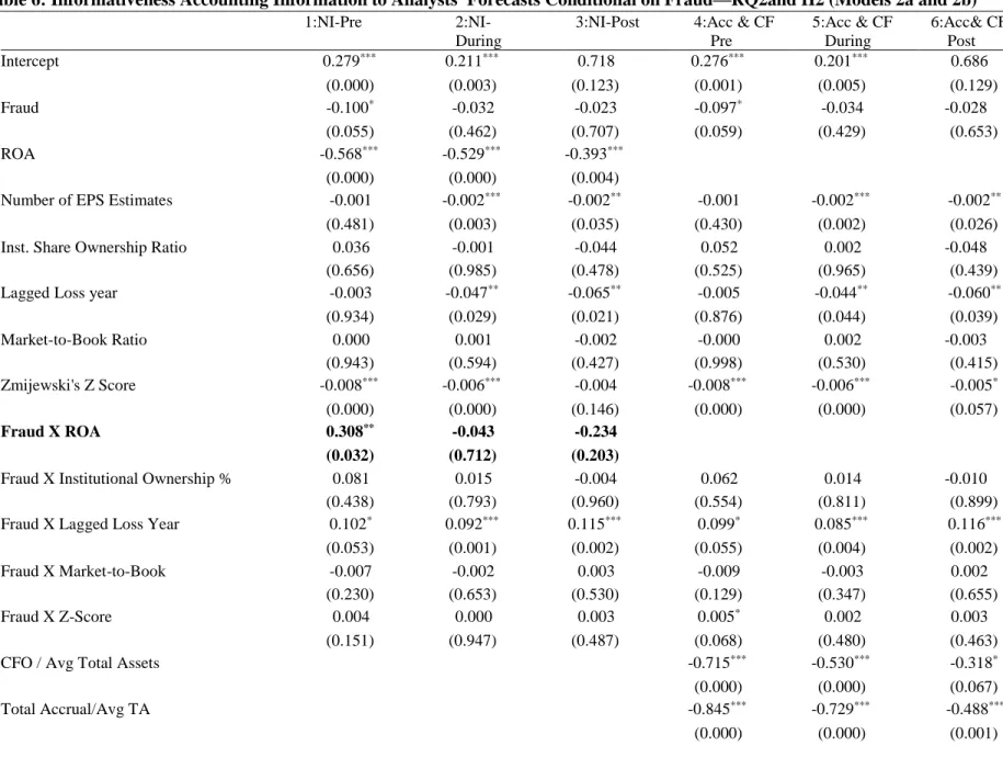
I evaluate RQ2 and H2 by estimating Model 2a and 2b to assess informativeness to analysts’ forecasts. The results of estimating Models 2a and 2b are in Table 6.
Table 6 shows that higher earning firms are associated with lower analysts’ forecast error as depicted in the negative coefficients on ROA across all three periods (all p-values <1%). However, conditional on fraud, ROA is positively associated with larger forecast errors in the pre-fraud period; the coefficient on Fraud X ROA is positive and significant (p <5%). There is no difference between fraud and non-fraud firms during the fraud and post-fraud period in how ROA is
316
associated with forecast errors (p =.71 and .20, respectively). The lack of a difference between the two groups of firms in the fraud period supports H2.
Fraud firms sustaining losses are associated with higher analysts’ forecast errors across all three periods. When earnings (ROA) are broken into cash flow and accrual, with one exception, there are no differences across all three periods. The exception is cash flow in the pre-fraud period. In the pre-fraud period, fraud firms’ cash flows are positively associated with analysts’ forecast error though accruals are not. (Fraud X CFO) / Avg TA is positive and significant in Column 4 (p <5%, Table 6). This may reflect erratic cash flows of fraud firms, perhaps motivating some of them to commit fraud in the first place. It is also possible, even likely that, fraud firms engaged in earnings management in the pre-fraud period that contributed to a distortion of their information environment, resulting in larger analysts’ forecast errors. [see Table 6, pg 326]
Regarding other accounting information, Fraud X Lagged Loss is positive and significant across all three periods (p=.052, .001, and .002 for pre-fraud, during, and post-fraud periods, respectively; see Table 6), reflecting the difficulty of forecasting earnings for loss-making firms.
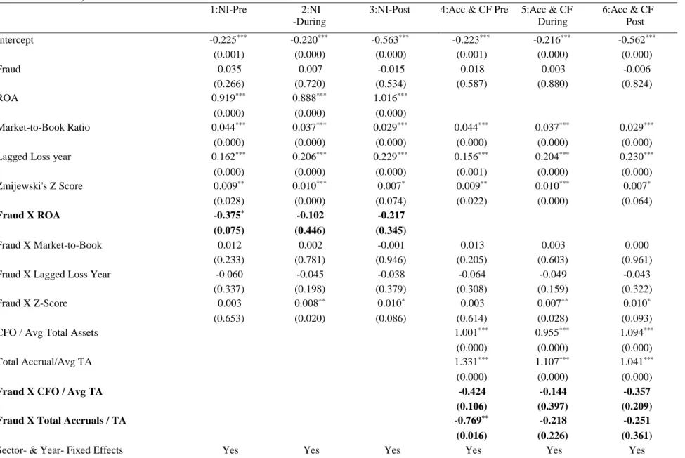
Informativeness of Accounting Information to Abnormal Returns (RQ3 and H3)
The results of estimating Models 3a and 3b are in Table 7. ROA and Market-to-Book ratio are positively associated with abnormal returns pre, during, and post fraud (all p-values <1%). Interestingly prior year losses (Lagged Loss) and Z-score are positively associated with abnormal returns across all three periods, though those of score are marginal (a higher Z-score implies greater financial distress). This phenomenon may reflect mean reversion in returns, correction from over-reaction to losses or a combination of these factors. Fraud firms with weak financial positions (measured by Fraud X Z-score) are marginally positively associated with excess returns in the fraud period but this association declines post-fraud (p-value <.03 during fraud period versus p-value <.10 post fraud). [see Table 7, pg 328]
Fraud firms experience marginally negative excess returns in the pre-fraud period but not in subsequent periods. Fraud X ROA is negative (p=.075, .446, and .345 pre, during, and post fraud periods respectively, in Table 7). The absence of a difference in the fraud period supports H3.
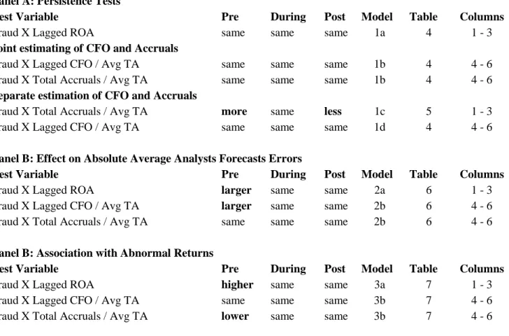
When net income (ROA) is decomposed into accruals and cash flows, both components are positively associated with excess return across all three periods (all p-values <1%; see last three columns of Table 7). However, the cash flows of fraud firms do not provide incremental excess returns, evidenced in the insignificant coefficient on (Fraud X CFO) / Avg TA (all p-values >10%; see last three columns of Table 7). The insignificant association of cash flows with excess returns conditional on fraud suggests the difficulty of disguising the quality of cash flows. On the other hand, Fraud X Accruals is negatively associated with excess returns pre-fraud (p <5%, Column 4, Table 7), but not during the fraud or post-fraud periods. Again, this suggests that the market is able to distinguish to some extent the quality of accruals in the pre-fraud period, consistent with Collins et al. (2003) who find that after the publishing of Sloan (1996) institutional investors have largely arbitraged away the accrual anomaly. However, this ability is perhaps attenuated by fraud. The absence of significant differences between fraud and non-fraud firms supports H3. Please see Figure 2 for a summary of the main results.
Discussion
These results suggest that fraud firms may have been motivated to commit fraud to help close the gap between them and their non-fraud peers in how their accounting information influences the financial markets. For example, the lack of significant difference in how accrual-based income influences analysts forecast errors coupled with the stronger association between accrual-based income and abnormal returns for non-fraud firms in the pre-fraud period suggests that the financial markets are quite good at distinguishing between higher quality firms (non-fraud) and lower quality firms (fraud) in that period.
These differences are mitigated during the fraud period. However, it is interesting that the differences largely do not return after the fraud period. It is possible that while the absence of a large number of significant differences during the fraud period could have been in part driven by fraud, it is not clear whether absence of differences in the post-fraud period is driven by better compliance with accounting and legal rules, better operating performance or both. Exploring the drivers of post fraud performance between fraud and peer non-fraud firms should be a fruitful area for future research. It is likely that in the post-fraud period, fraud firms’ compliance with accounting rules would improve, as would the strength of their controls. Coupling a stronger compliance and controls culture with better operational performance may be sufficient to erase
317
differences with non-fraud firms but it is not clear that a stronger compliance and controls environment alone would achieve that.
Conclusion
The paper evaluates the accounting information environments of fraud and non-fraud firms in terms of earnings persistence and informativeness to analysts’ earnings forecasts and abnormal returns and finds that with few exceptions, there are differences between the two groups before the fraud period, perhaps motivating the fraud in the first place. These differences tend to disappear during the fraud period, and there are no differences in returns after the fraud period.
In particular, fraud firms’ accruals tend to be more persistent pre-fraud but are indistinguishable from those of non-fraud firms during and post fraud. There are no differences in persistence of cash flow from operations between fraud and non-fraud firms pre, during, and post non-fraud. Fraud firms’ earnings are associated with larger forecast errors pre- non-fraud but not during and after the fraud period. When earnings are decomposed into cash flows and accruals, fraud firms’ cash flows are associated with larger analysts’ forecast errors pre-fraud, but the difference disappears during and post fraud.
Fraud firms’ earnings are associated with incrementally higher analysts’ earnings forecast errors pre-fraud, and most of that positive association derives from the cash flow component of earnings.
These differences in pre-fraud period accounting information environments of the two types of firms manifest in their returns. Fraud firms’ earnings are negatively associated with excess returns in the pre-fraud period, but this difference evaporates in the fraud and post-fraud periods. Perhaps reflecting the difficulty of manipulating cash, when earnings are decomposed into cash flows and accruals, cash flows are not associated with excess returns, but fraud firms’ accruals are negatively associated with excess returns in the pre-fraud period, suggesting that the financial markets discount the higher persistence of fraud firms’ accruals in the pre-fraud period.
These results have some implications for practice. Earnings by themselves are not very informative diagnostic tools for fraud but decomposing them into accrual and cash flows components can greatly enhance the researcher, investor, regulator or practitioner’s ability to diagnose potential fraud candidates. In particular, the results suggest that unusually high persistence of the accrual component of earnings can be a red flag, and more so if it is coupled with negative abnormal returns for the accrual component of earnings.
Furthermore, since accruals are more easily manipulated than cash, unusually large earnings forecast errors coupled with large forecast errors for the cash flows component of earnings for an extended period, followed by a period of consistently meeting or beating analysts’ earnings forecast can be a red flag. For practitioners without access to large data sets, a combination of temporal analyses of the firms of interest compared to the averages of a benchmark of peer firms would be a good starting point.
318
References
Barth, M.E., D.P. Cram, and K.K. Nelson. 2001. Accruals and the prediction of future cash flows.
Accounting Review, vol. 76, no. 1 (January): 27–58.
Beneish, M.D., Lee, C.M., and Nichols, D.C., 2013. Earnings manipulation and expected returns. Financial Analysts Journal.69 (2): 57–82.
Bhattacharya, N., E.L. Black, T.E. Christensen, and C.R. Larson. 2003. Assessing the relative informativeness and permanence of pro forma earnings and GAAP operating earnings. Journal of Accounting and Economics, 36(1– 3): 285–319.
Bhojraj, S., P. Hribar, and M. Piccomi. 2009. Making sense of cents: An examination of firms that marginally miss or beat analyst forecasts. The Journal of Finance 64.5 (2009): 2361–2388.
Bradshaw, M.T. and R.G. Sloan, 2002. GAAP versus the street: An empirical assessment of two alternative definitions of earnings. Journal of Accounting Research, 40(1):.41–66.
Carcello, J.V. and A.L. Nagy. 2004. Audit firm tenure and fraudulent financial reporting. Auditing: A Journal of Practice & Theory, 23(2): 55–69.
Collins, D., Gong, G., and Hribar, P., 2003. Investor sophistication and the mispricing of accruals. Review of Accounting Studies 8: 251–276.
Collins, D.W. and S.P. Kothari. 1989. An analysis of intertemporal and cross-sectional determinants of earnings response coefficients. Journal of Accounting and Economics, (nos. 2/3):143–181. Dechow, P.M. 1994. Accounting earnings and cash flows as measures of firm performance: The
role of accounting accruals. Journal of Accounting and Economics18(1): 3–42. Dechow, P.M. and I.D. Dichev. 2002. The quality of accruals and earnings: The role of accrual
estimation errors. Accounting Review, 77(Supplement): 35–59.
Dechow, P.M., S.P. Kothari, and Ross L. Watts. 1998. The Relation between earnings and cash flows. Journal of Accounting and Economics, 25(2):133–168.
Dechow, P., W. Ge, and C. Schrand. 2010. Understanding earnings quality: A review of the proxies, their determinants and their consequences. Journal of Accounting and Economics50(2): 344–401.
Dechow, P.M. and C M. Schrand. 2004. Earnings Quality. Research Foundation of the CFA Institute, 1–152. De Franco, G., S.P. Kothari, and R.S. Verdi. 2011. The benefits of financial statement
comparability. Journal of Accounting Research, 49(4): 895–931.
Desai, H., S. Rajgopal, and M. Venkatachalam. 2004. Value-glamour and accruals mispricing: One anomaly or two? The Accounting Review79(2): 355–385.
Duru, A. and D.M. Reeb. 2002. International diversification and analysts' forecast accuracy and bias. The Accounting Review, 77(2): 415–433.
Fairfield, P.M., J.S. Whisenant, and T.L. Yohn, 2003. Accrued earnings and growth: Implications for future profitability and market mispricing. The Accounting Review, 78(1):353–371.
Finger, C.A. 1994. The ability of earnings to predict future earnings and cash flows. Journal of Accounting Research, 32(2): 210–223.
Givoly, D., C.K. Hayn, and S.P. Katz. 2010. Does public ownership of equity improve earnings quality? The Accounting Review85(1): 195–225.
Glazer, E. 2016. Wells Fargo official in eye of storm. The Wall Street Journal, Tuesday, September 20, (Money and Investing): C1-C2.
319
Graham, J.R., C.R. Harvey, and S. Rajgopal. 2005. The economic implications of corporate financial reporting. Journal of Accounting and Economics40(1): 3–73.
Hayn, C. 1995. The information content of losses. Journal of Accounting and Economics20(2):125– 153.
Jones, J.F. 1991. Earnings management during import relief investigations. Journal of Accounting Research 29(2):193– 228.
McInnis, J. and D.W. Collins. 2011. The effect of cash flow forecasts on accrual quality and benchmark beating. Journal of Accounting and Economics51(3): 219–239.
Nelson, M.W., J.A. Elliott, and R.L. Tarpley. 2003. How are earnings managed? Examples from auditors. Accounting Horizons, 2003: 17–35.
Ohlson, J. and X.J. Zhang. 1998. Accrual accounting and equity valuation. Journal of Accounting Research 36(Supplement): 85–111.
Penman, S.H. and T. Sougiannis. 1998. A comparison of dividend, cash flow, and earnings approaches to equity valuation. Contemporary Accounting Research 15(3): 343–383.
Richardson, S.A. 2003. Earnings quality and short sellers. Accounting Horizons17(Supplement): 49–61. Skinner, D.J. and R.G. Sloan. 2002. Earnings surprises, growth expectations, and stock returns or
don’t let an earnings torpedo sink your portfolio. Review of Accounting Studies7(2/3): 289– 312.
Sloan, R.G. 1996. Do stock prices fully reflect information in accruals and Cash Flows about Future Earnings? Accounting Review, (3): 289–315.
Thomas, J.K. and H. Zhang. 2002. Inventory changes and future returns. Review of Accounting Studies7(2/3): 163–187.
Xie, H. 2001. The mispricing of abnormal accruals. Accounting Review76(3): 357–373.
Zmijewski, M.E. 1984. Methodological issues related to the estimation of financial distress prediction models. Journal of Accounting Research22(Supplement): 59–82.
320
Appendix Types of Fraud
The fraud of the following firms did not indicate any effect on the major financial statement items and so may not involve restatements. When the fraud occurred, and the description captured in the IFP database are outlined here:
Dow Chemical, 1996–2001, “bribed government official”; Bellsouth, 1997–2000, “No 10b-5 violation: paid bribes”; Haliburton, 1998–2006, “bribery of official within the Nigerian government”; DeGeorge Financial, 1992–1995, “failed to disclose personal expense”; Advanced Micro Devices, 1996–1996, “inaccurate and misleading statements in regards to the development of a 486 microprocessor”; Canadian Imperial Bank, 1998–2001, “manipulation of its reported financial results through a series of complex structured finance transactions”.
Matching Procedure
I identify matching non-fraudulent control firm by using the FASTCLUS procedure in SAS to find a match with the smallest Euclidean distance to a cluster of firms that are most similar to the fraud firm based on the variable of interest, size, and industry. The SAS FASTCLUS procedure uses disjoint cluster analysis in which each fraud firm belongs to one cluster only.
321
Table 1: Descriptive Statistics-Fraud Period
Mean 1st Quartile Median 3rd Quartile Std. Dev. ROA 0.02 -0.00 0.04 0.09 0.14
Lagged (NI/Avg TA) 0.01 0.00 0.03 0.07 0.11
CFO / Avg Asset 0.06 0.02 0.07 0.12 0.11
Lagged CFO/Avg TA ($Millions) 0.06 0.02 0.07 0.11 0.09
Lagged Total Accrual ($Millions) -456.25 -222.38 -24.57 -0.20 1,244.13
Total Accrual -482.33 -241.60 -31.18 -0.97 1,305.33
Lagged Loss Year 0.24 0.00 0.00 0.00 0.42
Lagged Operating Cashflow ($Millions) 794.17 3.52 55.05 393.08 2,031.19
Number of EPS Estimates 12.04 4.00 9.00 17.00 10.45
Inst. Share Ownership Ratio 0.54 0.33 0.56 0.76 0.26
Zmijewski's Z Score 3.96 1.27 2.82 5.04 4.68
Mean Forecast Error ($) -0.07 -0.08 0.00 0.06 0.33
Mean Abs.EPS Forecast Error (S) 0.19 0.02 0.07 0.19 0.35
Annual Cumulative Abnormal Return 0.03 -0.23 0.02 0.28 0.47
Market-to-Book Ratio 3.00 1.37 2.11 3.60 3.14
Inst. Share Ownership Ratio 0.54 0.33 0.56 0.76 0.26
Fraud 0.52 0.00 1.00 1.00 0.50
N 6,126
322
Table 2: Mean and Median Difference Tests-Fraud Period
Mean (Fraud Sample) Mean (Control Sample) p-value Median (Fraud Sample) Median (Control Sample) p-value ROA 0.01 0.03 0.00 0.04 0.04 0.00
Lagged (NI/Avg TA) 0.00 0.02 0.00 0.03 0.04 0.00
CFO / Avg Asset 0.05 0.08 0.00 0.06 0.08 0.00
Lagged CFO/Avg TA 0.05 0.07 0.00 0.06 0.08 0.00
Lagged Total Accrual ($Millions) -485.02 -424.90 0.06 -21.58 -28.14 0.03 Total Accrual ($Millions) -513.05 -448.86 0.05 -27.43 -34.30 0.04
Lagged Loss Year 0.26 0.20 0.00 0.00 0.00 0.00
Lagged Operating Cashflow ($Millions) 808.56 778.50 0.56 47.84 64.30 0.00
Number of EPS Estimates 12.48 11.56 0.00 10.00 8.00 0.00
Inst. Share Ownership Ratio 0.58 0.51 0.00 0.61 0.52 0.00
Zmijewski's Z Score 3.83 4.11 0.02 2.84 2.80 0.65
Mean Forecast Error ($) -0.08 -0.06 0.02 0.01 0.00 0.04
Mean Abs.EPS Forecast Error ($) 0.20 0.19 0.20 0.07 0.07 0.80
Annual Cumulative Abnormal Return 0.05 0.01 0.00 0.02 0.01 0.12
Market-to-Book Ratio 3.10 2.88 0.01 2.17 2.07 0.03
Inst. Share Ownership Ratio 0.58 0.51 0.00 0.61 0.52 0.00
Fraud 1.00 0.00 . 1.00 0.00 .
N 6,126
323
Table 3: Correlation of Primary Variables
ROA, 1 1
Lagged ROA, 2 0.55** 1
CFO / Avg TA, 3 0.53** 0.45** 1
Lagged CFO /Avg TA, 4 0.42** 0.54** 0.63** 1
Total Accrual / Avg TA, 5 0.43** 0.14** -0.45** -0.19** 1
Lagged Total / Avg TA, 6 0.12** 0.42** -0.20** -0.49** 0.33** 1 Lagged Loss Year, 7 -0.40** -0.70** -0.29** -0.33** -0.13** -0.37** 1 Number of EPS Estimates, 8 0.15** 0.20** 0.27** 0.28** -0.10** -0.08** -0.14** 1 Inst. Share Ownership Ratio, 9 0.13** 0.11** 0.17** 0.14** -0.01 -0.02 0.14** 0.33** 1 Zmijewski's Z-Score, 10 0.18** 0.09** 0.08** 0.02 0.11** 0.07** 0.03 -0.03 0.05* 1 Mean Abs. EPS Forecast Error, 11 -0.20** -0.10** -0.06** -0.07** -0.17** -0.03 0.11** -0.04 -0.01 0.18** 1 Annual Cumulative Abnormal Returns, 12 0.23** -0.03 0.12** 0.02 0.10** -0.04* 0.01 0.01 0.12** 0.27** -0.11**
Market-to-Book Ratio, 13 0.11** 0 0.07** 0.02 0.01 0 0.03 0.12** 0.03 0.52** -0.14** Fraud, 14 -0.06* -0.08** -0.10** -0.11** 0.03 0.05* 0.06** 0.13** -.05* .04* 0.07**
Mean Abs. EPS Forecast Error, 11 1 Annual Cumulative Abnormal Returns,12 -0.11** 1 Market-to-Book Ratio, 13 -0.14** 0.38** 1 Fraud, 14 0.07** 0.02 0.13** 1
1 2 3 4 5 6 7 8 9 10 11
324
Table 4: Persistence of Earnings and its Decomposition into Accruals and Cash Flow Conditional on Fraud—RQ1 and H1 (Models 1a and 1b)
1:NI-Pre 2:NI
-During
3:NI-Post 4:Acc & CF -Pre 5:Acc & CF During 6:Acc & CF Post Intercept 0.021*** 0.016*** 0.018*** 0.006 -0.008* -0.008 (0.000) (0.000) (0.000) (0.253) (0.065) (0.178) Lagged ROA) 0.760*** 0.670*** 0.586*** (0.000) (0.000) (0.000) Fraud -0.007 -0.006 -0.001 -0.000 -0.001 -0.001 (0.283) (0.149) (0.914) (0.978) (0.901) (0.871)
Fraud X Lagged ROA 0.142 0.023 -0.059
(0.167) (0.691) (0.382)
Lagged CFO/Avg TA 0.930*** 0.891*** 0.800***
(0.000) (0.000) (0.000)
Lagged Total Accruals/Avg TA 0.648*** 0.504*** 0.426***
(0.000) (0.000) (0.000)
Fraud X Lagged CFO/Avg TA 0.082 0.022 -0.033
(0.459) (0.771) (0.715)
Fraud X Lagged Total Accruals/Avg TA 0.124 0.011 -0.107
(0.272) (0.854) (0.191)
N 2130 6126 2863 2130 6126 2863
Adj R-squared 0.308 0.296 0.290 0.315 0.319 0.319
Note: p-values in parentheses*p < 0.10, **p < 0.05, ***p < 0.01. The results of estimating Model 1a are in columns 1–3 while those of
estimating Model 1b are in columns 4–6. The lack of significance of Fraud X Lagged CFO/ Avg TA and Fraud X Lagged Total Accrual / Avg TA is in part driven by the highly negative correlation between CFO and Accruals (-0.19, see Table 3). Thus, both variables in the same model cancel each other out to some extent.
325
Table 5: Relative Persistence of Accruals and Cash Flow Conditional on Fraud—RQ1 and H1(Models 1c and 1d)
1:Acc-Pre 2: Acc
-During
3:Acc -Post 4: CFO -Pre 5:CFO -During 6:CFO-Post Intercept -0.028*** -0.039*** -0.041*** 0.027*** 0.026*** 0.028*** (0.000) (0.000) (0.000) (0.000) (0.000) (0.000) Fraud 0.009* 0.006* -0.006 -0.012* -0.011*** -0.002 (0.097) (0.084) (0.218) (0.060) (0.006) (0.711)
Lagged Total Accruals/Avg TA 0.313*** 0.290*** 0.287***
(0.000) (0.000) (0.000)
Fraud X Lagged Total Accruals/Avg TA 0.166** 0.049 -0.110**
(0.029) (0.237) (0.044)
Lagged CFO/Avg TA 0.725*** 0.730*** 0.703***
(0.000) (0.000) (0.000)
Fraud X Lagged CFO/Avg TA 0.108 0.061 -0.014
(0.160) (0.204) (0.804)
N 2130 6126 2863 2130 6126 2863
Adj R-squared 0.115 0.083 0.052 0.396 0.423 0.416
Note: p-values in parentheses. *p < 0.10, **p < 0.05, ***p < 0.001. The results of estimating Model 1c are in columns 1–3 while those of estimating Model 1d are in columns 4–6.
326
Table 6: Informativeness Accounting Information to Analysts' Forecasts Conditional on Fraud—RQ2and H2 (Models 2a and 2b)
1:NI-Pre 2:NI- 3:NI-Post 4:Acc & CF 5:Acc & CF 6:Acc& CF During Pre During Post
Intercept 0.279*** 0.211*** 0.718 0.276*** 0.201*** 0.686 (0.000) (0.003) (0.123) (0.001) (0.005) (0.129) Fraud -0.100* -0.032 -0.023 -0.097* -0.034 -0.028 (0.055) (0.462) (0.707) (0.059) (0.429) (0.653) ROA -0.568*** -0.529*** -0.393*** (0.000) (0.000) (0.004)
Number of EPS Estimates -0.001 -0.002*** -0.002** -0.001 -0.002*** -0.002**
(0.481) (0.003) (0.035) (0.430) (0.002) (0.026)
Inst. Share Ownership Ratio 0.036 -0.001 -0.044 0.052 0.002 -0.048
(0.656) (0.985) (0.478) (0.525) (0.965) (0.439)
Lagged Loss year -0.003 -0.047** -0.065** -0.005 -0.044** -0.060**
(0.934) (0.029) (0.021) (0.876) (0.044) (0.039) Market-to-Book Ratio 0.000 0.001 -0.002 -0.000 0.002 -0.003 (0.943) (0.594) (0.427) (0.998) (0.530) (0.415) Zmijewski's Z Score -0.008*** -0.006*** -0.004 -0.008*** -0.006*** -0.005* (0.000) (0.000) (0.146) (0.000) (0.000) (0.057) Fraud X ROA 0.308** -0.043 -0.234 (0.032) (0.712) (0.203)
Fraud X Institutional Ownership % 0.081 0.015 -0.004 0.062 0.014 -0.010
(0.438) (0.793) (0.960) (0.554) (0.811) (0.899)
Fraud X Lagged Loss Year 0.102* 0.092*** 0.115*** 0.099* 0.085*** 0.116***
(0.053) (0.001) (0.002) (0.055) (0.004) (0.002)
Fraud X Market-to-Book -0.007 -0.002 0.003 -0.009 -0.003 0.002
(0.230) (0.653) (0.530) (0.129) (0.347) (0.655)
Fraud X Z-Score 0.004 0.000 0.003 0.005* 0.002 0.003
(0.151) (0.947) (0.487) (0.068) (0.480) (0.463)
CFO / Avg Total Assets -0.715*** -0.530*** -0.318*
(0.000) (0.000) (0.067)
Total Accrual/Avg TA -0.845*** -0.729*** -0.488***
327
Fraud X CFO / Avg TA 0.468** -0.050 -0.140
(0.013) (0.732) (0.539)
Fraud X Total Accruals / Avg TA 0.249 -0.160 -0.289
(0.284) (0.306) (0.199)
Sector- & Year-Fixed Effects Yes Yes Yes Yes Yes Yes
N 2130 6126 2863 2130 6126 2863
Adj R-squared 0.135 0.136 0.165 0.146 0.146 0.166
Note: p-values in parentheses. *p < 0.10, **p < 0.05, ***p < 0.01. The results of estimating Model 2a are in columns 1–3 while those of estimating Model 2b
are in columns 4–6.
328
Table 7: Informativeness of Accounting Information to Annual Cumulative Abnormal Returns Conditional on Fraud—RQ3 and H3 (Models 3a and 3b)
1:NI-Pre 2:NI
-During
3:NI-Post 4:Acc & CF Pre 5:Acc & CF During 6:Acc & CF Post Intercept -0.225*** -0.220*** -0.563*** -0.223*** -0.216*** -0.562*** (0.001) (0.000) (0.000) (0.001) (0.000) (0.000) Fraud 0.035 0.007 -0.015 0.018 0.003 -0.006 (0.266) (0.720) (0.534) (0.587) (0.880) (0.824) ROA 0.919*** 0.888*** 1.016*** (0.000) (0.000) (0.000) Market-to-Book Ratio 0.044*** 0.037*** 0.029*** 0.044*** 0.037*** 0.029*** (0.000) (0.000) (0.000) (0.000) (0.000) (0.000)
Lagged Loss year 0.162*** 0.206*** 0.229*** 0.156*** 0.204*** 0.230***
(0.000) (0.000) (0.000) (0.001) (0.000) (0.000) Zmijewski's Z Score 0.009** 0.010*** 0.007* 0.009** 0.010*** 0.007* (0.028) (0.000) (0.074) (0.022) (0.000) (0.064) Fraud X ROA -0.375* -0.102 -0.217 (0.075) (0.446) (0.345) Fraud X Market-to-Book 0.012 0.002 -0.001 0.013 0.003 0.000 (0.233) (0.781) (0.946) (0.205) (0.603) (0.961)
Fraud X Lagged Loss Year -0.060 -0.045 -0.038 -0.064 -0.049 -0.043
(0.337) (0.198) (0.379) (0.308) (0.159) (0.322)
Fraud X Z-Score 0.003 0.008** 0.010* 0.003 0.007** 0.010*
(0.653) (0.020) (0.086) (0.614) (0.028) (0.093)
CFO / Avg Total Assets 1.001*** 0.955*** 1.094***
(0.000) (0.000) (0.000)
Total Accrual/Avg TA 1.331*** 1.107*** 1.041***
(0.000) (0.000) (0.000)
Fraud X CFO / Avg TA -0.424 -0.144 -0.357
(0.106) (0.397) (0.209)
Fraud X Total Accruals / TA -0.769** -0.218 -0.251
(0.016) (0.226) (0.361)
329
N 2130 6126 2863 2130 6126 2863
Adj R-squared 0.233 0.203 0.157 0.231 0.200 0.152
Note; p-values in parentheses. *p < 0.10, **p < 0.05, ***p < 0.01. The results of estimating Model 3a are in columns 1–3 while those of estimating Model 3b
are in columns 4–6.
330
Figure 1: Data Procedure and Composition of Final sample
Initial IFP data 834 fraud firm years
Observations for which data is available 728 fraud firm years Observations for which there are matching non-fraud control firms 658 fraud firm years
Breakdown of final sample across the three periods after extracting financial data for both fraud and control firms
Fraud Period
Fraud firm-years Control firm-years Total
3,194 2,932 6,126
Pre-fraud Period
Fraud firm-years Control firm-years Total
1,077 1,053 2,130
Post-fraud Period
Fraud firm-years Control firm-years Total
1,477 1,386 2,863
Total
Fraud firm-years Control firm-years Total
331
Figure 2: Summary of Results—Effect of Fraud versus Control (Non-fraud) on
Earnings Quality
Panel A: Persistence Tests
Test Variable Pre During Post Model Table Columns
Fraud X Lagged ROA same same same 1a 4 1 - 3
Joint estimating of CFO and Accruals
Fraud X Lagged CFO / Avg TA same same same 1b 4 4 - 6
Fraud X Total Accruals / Avg TA same same same 1b 4 4 - 6
Separate estimation of CFO and Accruals
Fraud X Total Accruals / Avg TA more same less 1c 5 1 - 3
Fraud X Lagged CFO / Avg TA same same same 1d 4 4 - 6
Panel B: Effect on Absolute Average Analysts Forecasts Errors
Test Variable Pre During Post Model Table Columns
Fraud X Lagged ROA larger same same 2a 6 1 - 3
Fraud X Lagged CFO / Avg TA larger same same 2b 6 4 - 6
Fraud X Total Accruals / Avg TA same same same 2b 6 4 - 6
Panel B: Association with Abnormal Returns
Test Variable Pre During Post Model Table Columns
Fraud X Lagged ROA higher same same 3a 7 1 - 3
Fraud X Lagged CFO / Avg TA same same same 3b 7 4 - 6