VCU Scholars Compass
VCU Scholars Compass
Theses and Dissertations Graduate School
2020
Multi-label classification models for heterogeneous data: an
Multi-label classification models for heterogeneous data: an
ensemble-based approach.
ensemble-based approach.
Jose Maria Moyano Murillo
Virginia Commonwealth University
Follow this and additional works at: https://scholarscompass.vcu.edu/etd Part of the Computer Sciences Commons
© Jose Maria Moyano Murillo
Downloaded from Downloaded from
https://scholarscompass.vcu.edu/etd/6431
This Dissertation is brought to you for free and open access by the Graduate School at VCU Scholars Compass. It has been accepted for inclusion in Theses and Dissertations by an authorized administrator of VCU Scholars Compass. For more information, please contact [email protected].
Virginia Commonwealth University, USA
Multi-label classification models
for heterogeneous data:
an ensemble-based approach
Modelos de clasificación multi-etiqueta para datos heterogéneos: un enfoque basado en ensembles
by
Jose María Moyano Murillo
Ph.D. CandidateAdvisors:
Dr. Eva L. Gibaja
Dr. Sebastián Ventura
Dr. Krzysztof J. Cios
Department of Computer Science
and Numerical Analysis Department of Computer Science
University of Córdoba Virginia Commonwealth University
A Dissertation submitted in partial fulfillment of the requirements for the degree of Doctor of Philosophy with a concentration in Computer Science at
University of Córdoba (Computación Avanzada, Energía y Plasmasprogram)
and Virginia Commonwealth University. May 2020
Córdoba, May 2020
Ph.D. Candidate
Jose María Moyano Murillo
Advisor Advisor Advisor
Dr. Eva L. Gibaja Dr. Krzysztof J. Cios Dr. Sebastián Ventura
i
an ensemble-based approach”, reported by Jose María Moyano Murillo to qualify for the doctoral degree, has been conducted under the “Computación Avanzada, En-ergía y Plasmas” program at University of Córdoba and the program “Engineering, Doctor of Philosophy (Ph.D.) with a concentration in computer science/Computer Science Ph.D. with the University of Cordoba” at Virginia Commonwealth Univeristy, under the supervision of the doctors Eva Lucrecia Gibaja Galindo (University of Córdoba), Krzysztof J. Cios (Virginia Commonwealth University), and Sebastián Ventura Soto (University of Córdoba) fulfilling, in their opinion, the requirements
demanded by this type of works and respecting the rights of other authors to be
Córdoba, Mayo de 2020
Doctorando
Jose María Moyano Murillo
Director Director Director
Dr. Eva L. Gibaja Dr. Krzysztof J. Cios Dr. Sebastián Ventura
iii
neos: un enfoque basado en ensembles”, presentado por Jose María Moyano Murillo para optar al grado de doctor, ha sido realizado dentro del programa dual de doctor-ado en “Computación Avanzada, Energía y Plasmas” en la Universidad de Córdoba, y el programa “Engineering, Doctor of Philosophy (Ph.D.) with a concentration in computer science/Computer Science Ph.D. with the University of Cordoba” de la Virginia Commonwealth University, bajo la dirección de los doctores Eva Lucrecia Gibaja Galindo(UniversidaddeCórdoba),KrzysztofJ.Cios(Virginia Commonwealth
University), y Sebastián Ventura Soto (Universidad de Córdoba) cumpliendo, en su opinión, los requisitos exigidos a este tipo de trabajos y respetando los derechos de otros autores a ser citados, cuando se han utilizado sus resultados o publicaciones.
ensembles.
DOCTORANDO/A:
Jose María Moyano Murillo
Córdoba, 27 de Mayo de 2020
Firma del/de los director/es
Fdo.: Fdo.: Fdo.:
Conference on Artificial Intelligence o el IEEE Congress on Evolutionary Computation. Por último, presentación en varios congresos científicos de prestigio internacional, tales como la European
Es de destacar también que el trabajo de investigación desarrollado ha sido aceptado para su comportan. Este segundo modelo se ha publicado en la revista Knowledge-Based Systems. Tras el proceso de evolución, se obtiene un ensemble combinado los individuos que mejor se evolutivo con un enfoque diferente. En este caso, cada individuo codifica una parte del ensemble. la revista Information Fusion. Con posterioridad a este modelo, se desarrolló un segundo modelo algoritmos que integran el estado del arte. Dicho modelo dio lugar a una segunda publicación en
ensemble completo. El modelo produjo muy buenos resultados, siendo competitivo con los el desarrollo de un primer modelo propio, basado en un algoritmo evolutivo, que codificaba un revisión fue publicada en la revista Information Fusion. Posteriormente, se comenzó a trabajar en reglas que permitan la mejor elección posible de modelos en determinadas circunstancias. Esta multi-etiqueta, que permitiera una mejor comprensión del estado del arte, así como establecer de revisión para mostrar una taxonomía de los distintos modelos de ensembles para clasificación satisfactorio, como bien justifican los resultados obtenidos. Se comenzó trabajando en un artículo El trabajo realizado por el doctorando durante todo el periodo de investigación ha sido muy
(se hará mención a la evolución y desarrollo de la tesis, así como a trabajos y publicaciones derivados de la misma).INFORME RAZONADO DEL/DE LOS DIRECTOR/ES DE LA TESIS
Por todo ello, se autoriza la presentación de la tesis doctoral. trabajo.
calificarse de sobresaliente y que reúne con creces los requisitos exigibles a este tipo de Por todo lo comentado, consideramos que el trabajo presentado por D. José María Moyano puede codirector de esta tesis.
una estancia de seis meses en dicha Universidad, bajo la supervisión del Dr. Krzysztof Cios, Inteligencia Artificial de la Virginia Commonwealth University, habiendo realizado el candidato indicar que esta tesis doctoral se realiza en cotutela con el Dpto. de Ciencias de la Computación e
omy and Competitiveness and the European Regional Development Fund (FEDER), with projectsTIN2014-55252-PandTIN2017-83445-P, as well as by the Spanish
Min-istry of Education under FPU GrantFPU15/02958. The stay at Virginia
Common-wealth University has been also funded by the Spanish Ministry of Education, grant
referenceEST18/00807, and University of Córdoba (resolution published inBOUCO
no. 2019/00213).
Writing these last words of the thesis, I am realizing how I have changed thor-ough the years since I started working in the KDIS group, back in 2012. Further-more, which seemed to be a long period when I started the Ph.D. in 2016 comes to an end, and I am very pleased to have reached this objective. All the people in following lines have contributed to make me who I am today.
First, I would like to thank every single one of my advisors. Sebastián and Eva gave me the opportunity to start a research career many years ago, even when I did not know which it entailed. Thanks for discovering me a field that I really enjoy. Krys, thanks for helping me during the stay at VCU, in which I have learned a lot.
To the rest of people I have met in Richmond, Venant, Paolo, Javi, Chathu, and Dani. You made these months go faster and far more enjoyable. It will always be in my mind as good memories.
To all the people in the lab, who have not been few during all these years. Prob-ably, trying to name all of you I would miss someone, but you make work days funnier, with an excellent working atmosphere. You guys are definitely friends beyond the lab.
To my family, who have been always supporting me and being proud of what I achieve. Thank you very much.
And last but not least, to Lucia. You not only accompany me everyday, but you also support me in everything I do and, far more important, motivate me to keep fighting for my goals and working hard. Thanks for your smiles and for every little dumb thing. And thank you for bringing Venus into our lives. I love you.
”Todo acto de bondad es una demostración de poderío”. Miguel de Unamuno.
In recent years, the multi-label classification task has gained the attention of the scientific community given its ability to solve real-world problems where each in-stance of the dataset may be associated with several class labels simultaneously. For example, in medical problems each patient may be affected by several diseases at the same time, and in multimedia categorization problems, each item might be related with different tags or topics. Thus, given the nature of these problems, deal-ing with them as traditional classification problems where just one class label is assigned to each instance, would lead to a lose of information. However, the fact of having more than one label associated with each instance leads to new classifica-tion challenges that should be addressed, such as modeling the compound depen-dencies among labels, the imbalance of the label space, and the high dimensionality of the output space.
A large number of methods for multi-label classification has been proposed in the literature, including several ensemble-based methods. Ensemble learning is a technique which is based on combining the outputs of many diverse base models, in order to outperform each of the separate members. In multi-label classification, ensemble methods are those that combine the predictions of several multi-label classifiers, and these methods have shown to outperform simpler multi-label clas-sifiers. Therefore, given its great performance, we focused our research on the study of ensemble-based methods for multi-label classification.
The first objective of this dissertation is to perform an thorough review of the state-of-the-art ensembles of multi-label classifiers. Its aim is twofold: I) study dif-ferent ensembles of multi-label classifiers proposed in the literature, and catego-rize them according to their characteristics proposing a novel taxonomy; and II) perform an experimental study to find the method or family of methods that per-forms better depending on the characteristics of the data, as well as provide then some guidelines to select the best method according to the characteristics of a given problem.
Since most of the ensemble methods for multi-label classification are based on xiii
bels, our second and main objective is to propose novel ensemble methods for multi-label classification where the characteristics of the data are taken into ac-count. For this purpose, we first propose an evolutionary algorithm able to build an ensemble of multi-label classifiers, where each of the individuals of the popula-tion is an entire ensemble. This approach is able to model the relapopula-tionships among the labels with a relative low complexity and imbalance of the output space, also considering these characteristics to guide the learning process. Furthermore, it looks for an optimal structure of the ensemble not only considering its predictive performance, but also the number of times that each label appears in it. In this way, all labels are expected to appear a similar number of times in the ensemble, not neglecting any of them regardless of their frequency.
Then, we develop a second evolutionary algorithm able to build ensembles of multi-label classifiers, but in this case each individual of the population is a hypo-thetical member of the ensemble, and not the entire ensemble. The fact of evolv-ing members of the ensemble separately makes the algorithm less computationally complex and able to determine the quality of each member separately. However, a method to select the ensemble members needs to be defined. This process selects those classifiers that are both accurate but also diverse among them to form the ensemble, also controlling that all labels appear a similar number of times in the final ensemble.
In all experimental studies, the methods are compared using rigorous exper-imental setups and statistical tests over many evaluation metrics and reference datasets in multi-label classification. The experiments confirm that the proposed methods obtain significantly better and more consistent performance than the state-of-the-art methods in multi-label classification. Furthermore, the second proposal is proven to be more efficient than the first one, given the use of separate classifiers as individuals.
En los últimos años, el paradigma de clasificación multi-etiqueta ha ganado aten-ción en la comunidad científica, dada su habilidad para resolver problemas reales donde cada instancia del conjunto de datos puede estar asociada con varias etique-tas de clase simultáneamente. Por ejemplo, en problemas médicos cada paciente puede estar afectado por varias enfermedades a la vez, o en problemas de cate-gorización multimedia, cada ítem podría estar relacionado con varias etiquetas o temas. Dada la naturaleza de estos problemas, tratarlos como problemas de clasi-ficación tradicional donde cada instancia puede tener asociada únicamente una etiqueta de clase, conllevaría una pérdida de información. Sin embargo, el hecho de tener más de una etiqueta asociada con cada instancia conlleva la aparición de nuevos retos que deben ser abordados, como modelar las dependencias entre eti-quetas, el desbalanceo de etieti-quetas, y la alta dimensionalidad del espacio de salida. En la literatura se han propuesto un gran número de métodos para clasificación
multi-etiqueta, incluyendo varios basados enensembles. El aprendizaje basado en
ensemblescombina las salidas de varios modelos más simples y diversos entre sí, de cara a conseguir un mejor rendimiento que cada miembro por separado. En
clasifi-cación multi-etiqueta, se consideranensemblesaquellos métodos que combinan las
predicciones de varios clasificadores multi-etiqueta, y estos métodos han mostrado conseguir un mejor rendimiento que los clasificadores multi-etiqueta sencillos. Por tanto, dado su buen rendimiento, centramos nuestra investigación en el estudio de
métodos basados enensemblespara clasificación multi-etiqueta.
El primer objetivo de esta tesis el realizar una revisión a fondo del estado del arte en ensembles de clasificadores multi-etiqueta. El objetivo de este estudio es doble: I) estudiar diferentesensemblesde clasificadores multi-etiqueta propuestos en la literatura, y categorizarlos de acuerdo a sus características proponiendo una nueva taxonomía; y II) realizar un estudio experimental para encontrar el método o familia de métodos que obtiene mejores resultados dependiendo de las caracterís-ticas de los datos, así como ofrecer posteriormente algunas guías para seleccionar el mejor método de acuerdo a las características de un problema dado.
dos en la creación de miembros diversos seleccionando aleatoriamente instancias, atributos, o etiquetas; nuestro segundo y principal objetivo es proponer nuevos
modelos deensemblepara clasificación multi-etiqueta donde se tengan en cuenta
las características de los datos. Para ello, primero proponemos un algoritmo
evo-lutivo capaz de generar unensemblede clasificadores multi-etiqueta, donde cada
uno de los individuos de la población es unensemblecompleto. Este enfoque es ca-paz de modelar las relaciones entre etiquetas con una complejidad y desbalanceo de etiquetas relativamente bajos, considerando también estas características para
guiar el proceso de aprendizaje. Además, busca una estructura óptima para el
en-semble, no solo considerando su capacidad predictiva, pero también teniendo en cuenta el número de veces que aparece cada etiqueta en él. De este modo, se es-pera que todas las etiquetas aparezcan un número de veces similar en elensemble, sin despreciar ninguna de ellas independientemente de su frecuencia.
Posteriormente, desarrollamos un segundo algoritmo evolutivo capaz de con-struirensemblesde clasificadores multi-etiqueta, pero donde cada individuo de la
población es un hipotético miembro delensemble, en lugar delensemblecompleto.
El hecho de evolucionar los miembros delensemblepor separado hace que el
algo-ritmo sea menos complejo y capaz de determinar la calidad de cada miembro por separado. Sin embargo, también es necesario definir un método para seleccionar
los miembros que formarán elensemble. Este proceso selecciona aquellos
clasifi-cadores que sean tanto precisos como diversos entre ellos, también controlando que todas las etiquetas aparezcan un número similar de veces en elensemblefinal. En todos los estudios experimentales realizados, los métodos han sido compara-dos utilizando rigurosas configuraciones experimentales y test estadísticos, involu-crando varias métricas de evaluación y conjuntos de datos de referencia en clasi-ficación multi-etiqueta. Los experimentos confirman que los métodos propuestos obtienen un rendimiento significativamente mejor y más consistente que los méto-dos en el estado del arte. Además, se demuestra que el segundo algoritmo prop-uesto es más eficiente que el primero, dado el uso de individuos representando clasificadores por separado.
The Spanish legislation for Ph.D. studies, RD 99/2011, published on January 28th, 2011 (BOE-A-2011-2541), grants each Spanish University competencies to establish the necessary supervision and evaluation procedures to guarantee the quality of Ph.D. theses.
Accordingly, the University of Córdoba has a specific regulation for Ph.D. stud-ies, approved on December 21st, 2011. This regulation establishes two different modalities to elaborate the dissertation that the student has to present at the end of the doctorate studies. This Ph.D. thesis follows the modality described in the article no. 24 of the aforementioned regulation, referred as Ph.D. thesis as a compendium of publications. According to that article, the Ph.D. thesis can be presented as a com-pendium of, at least, three research articles published (or accepted for publication) in research journals of high quality, i.e. appearing in the first three quartiles of the Journal Citation Reports (JCR). If such a requirement is fulfilled, the manuscript has to include: an introduction to justify the thematic cohesion of the Ph.D. Thesis; the hypotheses and objectives to be achieved, and how they are associated to the publications; full copy of the publications; and conclusions.
Following these guidelines, this Ph.D. thesis is organized as follows. First, Chap-ter 1introduces the dissertation, including background and state-of-the-art work in topics related with the thesis. Next, the objectives and motivations are presented in Chapter 2, indicating which of the journal papers associated with the thesis fulfill each of the objectives. Later,Chapters 3to5present the main contributions of the thesis. In order to enhance the cohesion of the document, each of these chapters is divided in two parts: first, a brief introduction of the objectives, methodology, and conclusions of the corresponding study are presented; and then, the journal
paper is directly included. Chapter 6discusses the conclusions obtained thorough
the dissertation as well as presents some lines and future work. Finally, in Chap-ter 7, other publications associated with this Ph.D. thesis are included. At the end of the document, theVitaof the Ph.D. candidate is also provided.
Acronym Meaning
avgIR Average Imbalance Ratio
BP-MLL Back-Propagation for Multi-Label Learning
BR Binary Relevance
Card Cardinality
CBMLC Clustering-Based for Multi-Label Classification
CC Classifier Chains
CCEA Cooperative CoEvolutionary Algorithm
CDE Chi-Dep Ensemble
D3C Dynamic selection and Circulating Combination-based
Clustering
Dim Dimensionality
Div Diversity
DNF Did Not Finish
EA Evolutionary Algorithm
EAGLET Evolutionary AlGorithm for multi-Label Ensemble
opTi-mization
EBR Ensemble of Binary Relevances
ECC Ensemble of Classifier Chains
ELP Ensemble of Label Powersets
EME Evolutionary Multi-label Ensemble
EMLC Ensemble of Multi-Label Classifiers
EMLS Ensemble of Multi-Label Sampling
EPS Ensemble of Pruned Sets
ExAcc Example-based Accuracy
ExF Example-based FMeasure
ExP Example-based Precision
ExR Example-based Recall
ExS Example-based Specificity
GACC Genetic Algorithm for ordering Classifier Chains
G3P Grammar-Guided Genetic Programming
GA Genetic Algorithm
GEP Gene Expression Programming
GP Genetic Programming
GPL GNU General Public License
HL Hamming Loss
HOMER Hierarchy Of Multi-label classifiERs
IBLR-ML Instance-Based learning by Logistic Regression for
Multi-Label classification
LIFT Label specIfic FeaTures for multi-label learning
LP Label Powerset
MaAcc Macro-averaged Accuracy
MaF Macro-averaged FMeasure
MaP Macro-averaged Precision
MaR Macro-averaged Recall
MaS Macro-averaged Specificity
MiAcc Micro-averaged Accuracy
MiF Micro-averaged FMeasure
MiP Micro-averaged Precision
MiR Micro-averaged Recall
MiS Micro-averaged Specificity
MLC Multi-Label Classification
MLDA Multi-Label Dataset Analyzer
ML-ELM-RBF Multi-Layer Extreme Learning Machine of Radial Basis
Functions
ML-kNN Multi-Label k-Nearest Neighbors
MLL Multi-Label Learning
MLS Multi-Label Stacking
MLSOL Multi-Label Synthetic Oversampling based on the Local
distribution
PCT Predictive Clustering Tree
PS Pruned Sets
PSO Particle Swarm Optimization
RAkEL RAndom k-labELsets
rDep Ratio of Dependent labels pairs
RF-PCT Random Forest of Predictive Clustering Trees
SA Subset Accuracy
TREMLC Triple Random Ensemble for Multi-Label Classification
Symbol Meaning
X Input space
Y Output (label) space
D Multi-label dataset
xi Set of input attributes forith instance
Yi Set of relevant labels forith instance
Yi Set of irrelevant labels forith instance
ˆ
Yi Predicted set of relevant labels forith instance
ˆ
Yi Predicted set of irrelevant labels forith instance
λl lth label
fl Frequency oflth label inD
m Number of instances
d Number of input attributes
q Number of labels
H Search space of models
h Predictive model
e Ensemble
ej jth member of the ensemble
n Number of classifiers in the ensemble
ˆ
b Bipartition provided by a model
bjl Bipartition provided by jth member of the ensemble for
lth label
t Threshold for ensemble prediction
amin Minimum number of times that each label should appear
in the ensemble
eV Expected number of votes or appearances for each label
in the ensemble
p Population of the EA
s Offspring individuals in the EA
ind Individual of the population in the EA
popSize Size of the population in the EA
G Maximum number of generations of the EA
nT Number of classifiers built in the EA
β Multiplier for fitness combination
ϕ Correlation coefficient between labels
k Size of thek-labelsets (subsets ofklabels)
α Significance level for statistical tests
∆ Operator that returns the symmetric difference between
two binary sets
JπK Operator that returns 1 if predicateπis true, and 0
other-wise
Contents
Abstract xiii
Resumen (Spanish) xv
Preface xvii
Acronyms and abbreviations xix
Notation xxiii 1 Introduction 1 1.1 Ensemble learning . . . 1 1.1.1 Building phase . . . 2 1.1.2 Prediction phase . . . 3 1.2 Multi-label classification . . . 4 1.2.1 Formal definition of MLC . . . 6 1.2.2 Main challenges to address in multi-label data . . . 7 1.2.3 Multi-label classification algorithms . . . 8 1.2.4 Datasets characterization metrics . . . 18 1.2.5 Multi-label datasets . . . 21 1.2.6 Evaluation metrics . . . 21 1.2.7 Software tools for multi-labeled data . . . 27 1.3 Evolutionary algorithms . . . 28
2 Motivation and objectives 33
4 Evolutionary approach to evolve a whole EMLC: EME 59
5 Evolutionary approach to evolve ensemble members: EAGLET 79
6 Discussion and conclusions 99
6.1 Concluding remarks . . . 99 6.1.1 Experimental review and categorization of EMLCs . . . 100 6.1.2 Evolving the entire ensemble as individual . . . 101 6.1.3 Evolving separate members of the ensemble . . . 102 6.1.4 Open-source code . . . 102 6.2 Future work . . . 103
7 Other publications associated with this Ph.D. thesis 107
7.1 MLDA: A tool for analyzing multi-label datasets . . . 109 7.2 Generating EMLCs using CCEAs . . . 115 7.3 Tree-shaped EMLC using G3P . . . 125
References 135
Vita 147
List of Tables
1.1 Example of multi-label dataset. . . 6 1.2 Summary of state-of-the-art MLC methods. . . 9 1.3 Datasets and their characteristics. . . 22 1.4 Confusion matrix. . . 25 2.1 Objectives of the Ph.D. thesis and research papers that satisfy them. . 34
List of Figures
1.1 Reasons why ensemble methods outperform single learners. . . 2
1.2 Example of traditional classification. . . 5 1.3 Example of multi-label classification. . . 6 1.4 BR transformation. . . 10 1.5 LIFT transformation. . . 11 1.6 CC transformation. . . 11 1.7 LP transformation. . . 12 1.8 PS transformation. . . 13 1.9 ChiDep transformation. . . 13 1.10 Main steps of EAs. . . 31 1.11 Operation of EAs along the iterations. . . 31
Introduction
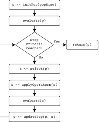
In this chapter we provide an introduction to the research topics on which this Ph.D. thesis is based. First, we provide a description of the ensemble learning framework, including main approaches to build ensembles (Section 1.1). Then, the Multi-Label Classification (MLC) paradigm is comprehensively explained (Sec-tion 1.2), including a formal defini(Sec-tion, state-of-the-art methods, characteriza(Sec-tion metrics, benchmark datasets, evaluation metrics to asses the performance of the methods, and an introduction to different multi-label libraries and tools . Finally, Evolutionary Algorithms (EAs), which are later used in our methodology, are de-scribed (Section 1.3).
1.1 Ensemble learning
When making crucial decisions, the tendency of humans is to gather information and opinions from different sources, then combining them into a final decision which is supposed to be better and more consistent than considering just one
opin-ion [1]. Based on this reasoning, ensemble learning is a machine learning
tech-nique which combines predictions of individual learners from heterogeneous or homogeneous modeling to obtain a combined learner that improves the overall generalization ability and reduces the overfitting of each [2,3].
Nowadays, ensemble methods are considered as the state-of-the-art to solve a wide range of machine learning problems, such as classification [4], regression [5], and clustering [6] problems. They have been successfully applied in fields such as finance [7], bioinformatics [8], medicine [9], and image retrieval [10].
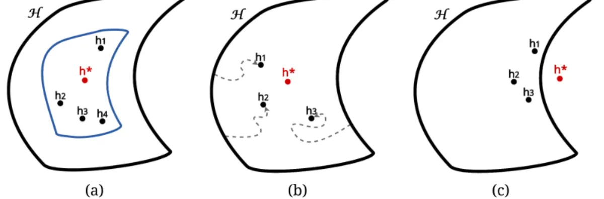
There are three main reasons why an ensemble learner use to perform better than single learners [11]. First, when picking only one single learner we run the risk of selecting one out of several learners that get same performance on training data, but which may perform different over unseen data; therefore, selecting some of these learners and combining their outputs, the optimal one, i.e., this which
per-forms better on unseen data, would be easily reached. InFigure 1.1a, the search
spaceHof models is indicated with the outer line, while the inner line denotes the set of learners that get the same performance in training, andh∗ denotes the op-timal learner. Second, many learning algorithms use local search to find a model and they may not find the optimal learner, so running several times the learning algorithm and combining the obtained models may result in a better approxima-tion to the optimal learner than any single one (Figure 1.1b). Third, since in most machine learning problems the optimal function might not be found, the optimal learner may be approximated by combining several feasible learners (Figure 1.1c).
(a) (b) (c)
Figure 1.1: Reasons why ensemble methods outperform single learners. (a) Com-bining several learners that perform similar on training data, the optimal one would be better reached. (b) Combining several learners obtained by local search could better reach the optimal learner. (c) Combining several feasible learners, the non-reachable optimal one could be better approximated.
1.1.1 Building phase
Although ensemble models tend to improve the generalization ability of base learn-ers, those learners to be combined into an ensemble should be carefully chosen. Using accurate learners seems to be an obvious approach; however, an ensemble including learners that are very similar to each other could not perform as well
as expected, and it may perform even worse than individual ones. Therefore, di-verse learners are usually preferred to be combined, although formal proof of this dependency does not exist [12,13].
The main approaches that have been proposed to build ensembles of diverse learners could be categorized in the following groups [1]:
Input manipulation Each base model is built over a slightly different subset of
the original training dataset (sampled with or without replacement). Thus, learners are diverse among them since each is focused on different input data.
Manipulated learning algorithm The way in which the learning algorithm
per-forms is modified. Usually, different hyperparameters are used for each en-semble member, such as using neural networks with different learning rates or number of layers, or support vector machines with different regularization parameters or kernels.
Partitioning The original dataset is divided in several mutually exclusive subsets, and each of them is used to train a different base learner. The original data can be split following two different approaches: a) horizontal partitioning, where each subset is composed of different instances (being non-overlapping subsets, unlike ininput manipulation); and b) vertical partitioning, where each member is built over all instances but each of them considering a different subset of the input attributes.
Output manipulation The output attribute (or attributes) is manipulated at each
of the members of the ensemble. Depending on the problem, the output at-tributes would be categorical classes, real-valued targets, etc.
Hybridization Usually, instead of just using one approach, two or even more
ap-proaches are hybridized in order to obtain far more diverse learners, aiming to improve the overall predictive performance of the ensemble learner.
1.1.2 Prediction phase
Given an ensemble modelecomposed bynbase learners, the final decision is made by combining individual predictions from each memberej, beingj∈[1, n]. Several approaches have been proposed in order to combine or integrate these predictions into the final one.
Weighting methods are the most usual techniques to combine predictions. These methods give a weight to each individual prediction, and then they are combined in any way. In particular, majority voting is the simplest and widely used weight-ing method, where the final prediction is the output with more votes among the base learners, or the average of predictions in real-valued outputs [5]. However, more complex approaches exist, such as giving a weight to each base learner based on their individual performance [14]; thus, the final prediction is biased by more accurate base learners while still considering all predictions.
On the other hand, instead of directly combining the predictions of individual learners, meta-learning methods build an ensemble in two-stages. In the first stage, several base learners are built and their predictions are gathered. Then, in a second phase, predictions of individual learners are used to build a meta-model, which may either extend the original input space with the predictions of previous stage, or just use these predictions as input attributes for the meta-model. Then, the output of the meta-model is used as the final ensemble prediction [15]. While weighting methods are better applicable in cases where the performance of base learners is similar, meta-learning methods are able to detect if certain base methods perform poorly in some subspaces.
1.2 Multi-label classification
Classification is one of the most popular and widely studied tasks in data mining. Traditional classification is a supervised learning task whose aim is to learn from data and their attributes to build a model that predicts the corresponding class for each of the instances. Whether binary (two classes) or multi-class (several classes), the main characteristic of traditional classification problems is that each of the
in-stances or examples is associated with one and only one class of the available ones.
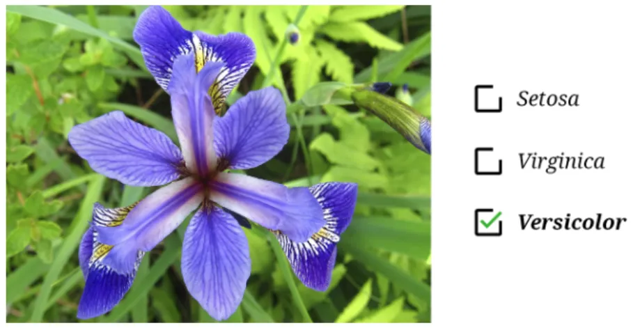
For example, as seen in Figure 1.2, each iris flower could belong to only one of
their species, eithersetosa, virginica, orversicolor, so the model predicts one of these classes given the characteristics of the flower [16].
Figure 1.2: Example of traditional classification.
However, there exist a large number of classification tasks where each exam-ple may have not only one but several classes or labels associated with it simul-taneously. For example, in multimedia annotation or text categorization prob-lems, each item could be categorized using several labels or topics [17,18]; in rec-ommender systems, the user may receive more than one recommendation at a
time [19]; in medical problems, patients may be affected by more than one
dis-ease [20]; and in biology, genes could be annotated with more than one function simultaneously [21]. MLC aims to build models to predict all the associated labels with each instance of the problem, and it has gained a lot of attention in the last decade [22].
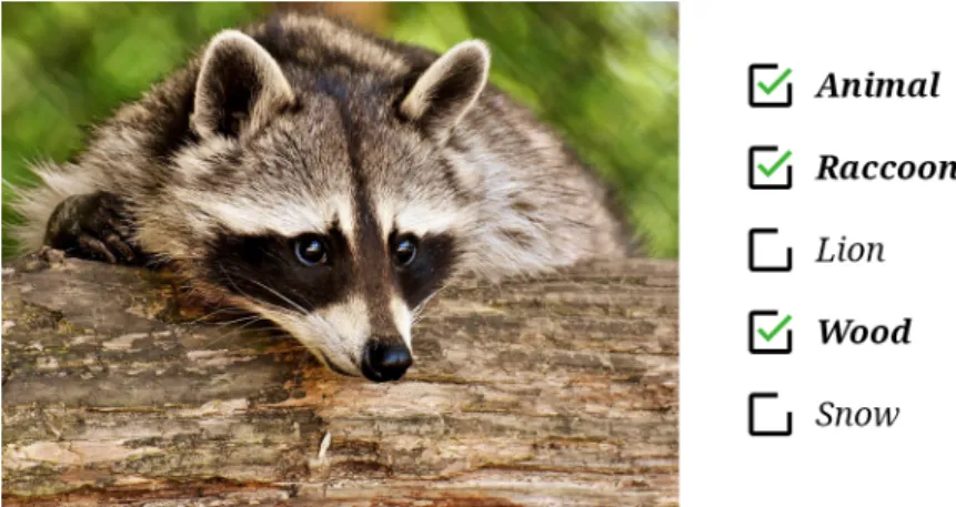
InFigure 1.3, the image can be annotated with several from previously defined labels, such asanimal,raccoon, andwood. As it can be observed, labels may be also related among them: ifraccoonlabel is present, theanimal label is very likely to be present too (although it does not need to be true in the other direction, i.e., the
appearance of theanimal label may not imply that the raccoon label is present),
but it is very unlikely to thesnowlabel to be relevant. Dealing with this image as a traditional classification problem (a.k.a. single-label classification), it would lead to a lose of information, since only one of the labels could be present.
Figure 1.3: Example of multi-label classification.
The MLC framework has been successfully applied to a large number of real-world problems, such as text categorization [23], multimedia annotation [24, 25, 26,27], bioinformatics [8,9, 28, 29], and social networks mining [30]. Therefore, the utility of the MLC paradigm in real-world problems have turned it into one of the hottest topics in data mining in the last years.
1.2.1 Formal definition of MLC
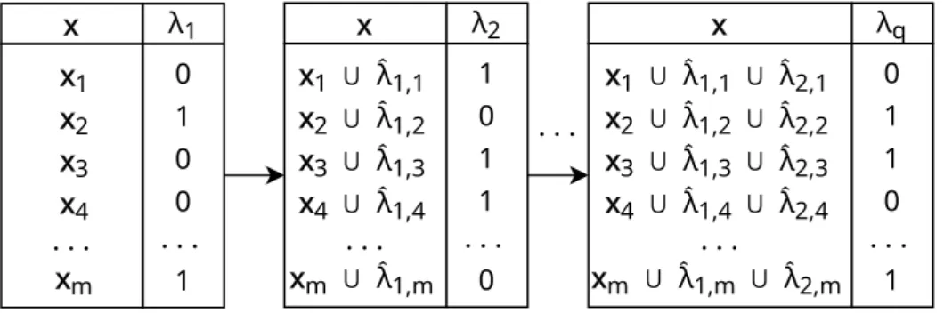
LetD be a multi-label dataset composed by a set of m instances, and defined as
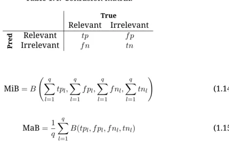
D ={(xi, Yi)|1 ≤ i ≤m}. LetX = X1× · · · ×Xdbe thed-dimensional input space, andY ={λ1, λ2, . . . , λq}the output space composed byq >1labels. Each multi-label instance is composed by an input vectorxi and a set of relevant labels associated with itYi ⊆ Y. Note that each differentY is also called labelset [22]. InTable 1.1, an example of multi-label dataset is shown. As seen, each example is labeled with one or more than one labels simultaneously.
Table 1.1: Example of multi-label dataset.
Instance Features Labels
λ1 λ2 λ3 . . . λq #1 x1 0 1 0 . . . 0 #2 x2 1 0 1 . . . 1 #3 x3 0 1 0 . . . 1 #4 x4 0 1 0 . . . 0 #5 x5 0 1 1 . . . 0 . . . . . . . . . #m xm 1 0 1 . . . 1
The goal of MLC is to construct a predictive modelh:X →2Y which provides a set of relevant labels for an unknown instance. Thus, for eachx∈ X, a bipartition ˆ b= ˆ Y ,Yˆ
of the label spaceY is provided, whereYˆ =h(x)is the set of relevant labels andYˆ the set of irrelevant ones. This bipartition could be also given as a binary vectorbˆ ={0,1}q, indicating if each label is relevant (1) or not (0).
Furthermore, lets define an Ensemble of Multi-Label Classifiers (EMLC) as a set ofnmulti-label classifiers. Each of the base classifiershj provides prediction ˆ
bj ={bj1,ˆ bj2, . . . ,ˆ bjqˆ }for all (or part of) the labels, eachbjbeing either1if the label is relevant and0otherwise. The final prediction of the ensemble is usually calcu-lated given the average value of the predictions for each labelvˆ = {v1,ˆ v2, . . . ,ˆ vqˆ}, where thevˆlfor each labelλlis calculated asvˆl= n1
Pn
j=1bˆjl. However, many other methods instead of simple voting could be used in order to combine predictions in the ensemble [31].
1.2.2 Main challenges to address in multi-label data
Given the fact that each instance of the data may have more than one label associ-ated, poses new challenges that need to be addressed, such as modeling the com-pound relationships among labels, the high dimensionality of the output space, and the imbalance of the output space.
Relationship among labels
As seen inFigure 1.3, output labels are not usually independent but they tend to be related to each other; e.g., a label may appear more frequently with some labels than with others. Thus, if the model is able to learn from these dependencies, its predictive performance would be improved. Consider that for a given instance, the learning method initially predicts justraccoon andwoodlabels as relevant ones. If the method models the relationship among labels, and it has learn that with a
very high probability when the raccoon label appears, the animal label appears
too, it would be able to amend its prediction and finally predict theanimal label too. However, not learning these dependencies would lead to a poorer predictive performance.
Considering the way in which the MLC methods address this problem, they are usually categorized as: I) first-order strategies, where labels are modeled com-pletely independent, and therefore the dependencies among labels are not learned; II) second-order strategies, where the dependencies among pairs of labels are taken into account; and III) high-order strategies, which model the dependencies among groups of more of two labels jointly [32].
Label imbalance
It is intrinsic to many problems that labels do not appear with the same frequency
in the dataset. For example, in the dataset containing the image in Figure 1.3,
maybe most of the instances have associated theanimal label, but less have the
raccoonone, and just a very small percentage of images are assigned thesnow
la-bel. Thus, if thesnowlabel barely appear in the dataset and the learning algorithm does not control this imbalance, it may be despised and the final method could not be able to predict it correctly.
The fact of having a lot of information for some labels but very little information of some others, leads to the difficulty of learning the infrequent ones. The task of learning from imbalanced datasets has been widely tackled in the literature; however, in multi-label scenarios, it should be addressed differently due to the high number of output labels.
Dimensionality of the output space
In multi-label scenarios, the dimensionality of the dataset is not only related to the number of instances and/or attributes as in many machine learning tasks, but also to the number of output labels. Problems with a low number of labels are easier to tackle, but in cases with a complex output space, the problem becomes far more difficult to be solved.
For example, it is much easier to learn the dependencies among labels if there are just six labels rather than a hundred labels. So, the dimensionality of the output space should be carefully considered in order to not to have extremely complex models.
1.2.3 Multi-label classification algorithms
In this section we introduce state-of-the-art methods in MLC, which are categorized into three main groups: problem transformation (PT), algorithm adaptation (AA), and EMLCs [22,33]. Note that not all methods are able to deal with each of the problems or characteristics of multi-labeled data (such as imbalance, relationship among labels, and high dimensionality of the output space); for example, some are not able to learn from the dependencies among labels in any way to enhance the final prediction. Furthermore, several of those that are able to deal with any char-acteristic, still do not consider it in their building phase, e.g., using the relationships among labels to lead the learning process, towards combinations of related labels
for example. InTable 1.2 a summary of the methods is provided, indicating for
each of them if they are able to deal with (D) and/or consider these characteristics in the building phase (B).
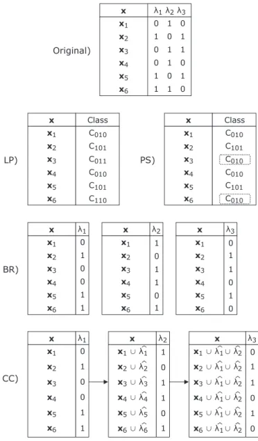
Problem transformation methods
Problem transformation methods transform a multi-label problem into one or sev-eral label problems, then solving each new problem using traditional single-label algorithms. For ease of understanding, and considering the multi-single-label dataset inTable 1.1, schemes of main transformations are presented.
One of the most popular methods is Binary Relevance (BR) [34] which
decom-poses the multi-label learning problem into q independent binary classification
problems, one for each label, as presented inFigure 1.4. The final multi-label pre-diction is obtained by combining the prepre-dictions of each single-label classifier. The fact that BR treats each label separately makes it simple, highly parallelizable, and resistant to overfitting label combinations, but it does not take into account label combinations so makes it unable to model possible dependencies among the labels. Thus, BR does not deal with any of the previously described problems in MLC.
Label specIfic FeaTures for multi-label learning (LIFT) [35] is based on the idea of modeling each label just considering their related input features, i.e., their label-specific features, thus avoiding the noise provided by features that are not
cor-Table 1.2: Summary of state-of-the-art MLC methods. It is indicated with a ‘D’ if the method is able to deal with the corresponding problem (imbalance, relation-ships among labels, and high dimensionality of the output space), and with a ‘B’ if it considers this characteristic at building phase.
Imbalance Relationships Output Dim.
PTs BR - - -CC - D -GACC - D, B -LIFT D, B - -LP - D -PS D, B D D, B ChiDep D D, B D, B AAs PCT - D, B -ML-kNN - D, B -IBLR-ML - D, B -BP-MLL - D, B -EMLCs EBR - - -ECC - D -MLS - D -HOMER D D, B D, B AdaBoost.MH - - -D3C - - -EPS D, B D D, B RAkEL D D D, B TREMLC D D D, B CDE D D, B D, B RF-PCT - D, B -CBMLC D D D EMLS D, B D -Figure 1.4: BR transformation.
related with them. For this purpose, LIFT uses clustering of the feature space to select a subset of features that best discriminate each label independently, and then builds a binary model for each of the labels. Figure 1.5 presents this trans-formation, where each binary classifier is also built over different subset of input features (xλl). In this process, LIFT considers the imbalance of the labels, being also able to deal with it; however, given the construction of independent models, it does not manage to deal neither with the relationship among labels nor the high dimensionality of the output space.
Figure 1.5: LIFT transformation.
In order to overcome the label independence assumption of BR, Classifier Chain (CC) [36] generatesq binary classifiers but linked in such a way that each binary classifier also includes the label predictions of previous classifiers in the chain as additional input features (Figure 1.6). In this way and unlike BR, CC is able to model the relationships among the labels without introducing more complexity. However, although it deals with the relationship among labels, it does not consider them, or any other characteristics of the data, at any moment of the building phase, such as to select the chain (which is randomly selected).
Since the order of the chain has a determinant effect on its performance, other approaches have been proposed to select the best chain ordering, as Genetic Al-gorithm for ordering Classifier Chains (GACC) [37]. GACC uses a genetic algorithm to select the most appropriate chain for CC. Each individual in GACC represents a label permutation, i.e., a chain for CC, and they are evaluated using a linear com-bination of three evaluation metrics. In this way, while GACC looks for an optimal chain ordering, it also considers the relationship among labels to build the model. Label Powerset (LP) [26] transforms the multi-label problem into a multi-class problem, creating one single-label dataset where each distinct labelset is consid-ered as a different class, as seen inFigure 1.7. Then, LP uses any multi-class clas-sification method to train a model with the new data, and the final prediction is obtained by transforming the predicted class to its corresponding labelset. LP con-siders all label correlations but its complexity is exponential with the number of labels. Furthermore, it is not able to predict a labelset that does not appear in the training dataset and, since many labelsets are usually associated with only few ex-amples, it may lead to a highly imbalanced dataset which would make the learning process more difficult and less accurate. Therefore, LP is able to deal with the rela-tionship among labels, but it increases the imbalance and the dimensionality of the output space, while it does not consider any of the characteristics when building the model.
Figure 1.7: LP transformation.
Pruned Sets (PS) [38] tries to reduce the complexity of LP, focusing on most im-portant combinations of labels by pruning instances with less frequent labelsets. To compensate for this loss of information, it then reintroduces the pruned instances with a more frequent subset of labels. Thus, PS considers the imbalance of LP’s
output space in its building phase to reduce its high dimensionality and complex-ity, although it might be still very complex in certain cases. Note that inFigure 1.8, labelsets appearing less than 2 times (as for instance #3) are pruned and reintro-duced with a more frequent subsets.
Figure 1.8: PS transformation.
ChiDep [39] (a.k.a. LPBR) creates groups of dependent labels based on theχ2test for labels dependencies identification [40]. For each group of dependent labels it builds a LP classifier, while for each single label which is not in any group it builds a binary classifier. In the example in Figure 1.9, since labels λ1 and λq are
cor-related they are modeled together with LP approach, while label λ2 for example
is modeled independently. ChiDep tries to reduce the disadvantages of the inde-pendence assumption of the binary methods and allows for simpler LP methods. Besides, ChiDep considers the relationship among group of labels and the dimen-sionality of the output space in building phase, therefore being able to reduce the imbalance in each model if the groups are small.
Algorithm adaptation methods
Algorithm adaptation methods utilized almost all single-label classification tech-niques to directly handle multi-label data. Therefore, it is not necessary to trans-form the dataset.
Predictive Clustering Trees (PCTs) [41] are decision trees that can be viewed as a hierarchy of clusters; the root node of the PCT tree contains all data, and it is re-cursively partitioned into smaller clusters in children nodes. These trees are able to deal with multi-label data since the distance between two instances for the clus-tering algorithm is defined as the sum of Gini Indexes [42] of all labels; therefore it not only is able to model the relationship among labels but it also consider them in the building phase.
The well-known instance-based k-Nearest Neighbors (kNN) method has been
also adapted to MLC. Multi-Label k-Nearest Neighbors (ML-kNN) [43] deals with
multi-label data by finding theknearest neighbors of a given instance, counting the
number of neighbors belonging to each label, and using themaximum a posteriori
principle to predict the labels for the given instance. As ML-kNN considers all label assignments of thek-nearest neighbors to label a new instance, it implicitly con-siders the relationship among labels to build the model. Besides, Instance-Based learning by Logistic Regression for Multi-Label classification (IBLR-ML) [44] is an-other example of adaptation of instance-based algorithms to MLC. It uses the la-bels of neighbor instances as extra input attributes in a logistic regression scheme. Therefore, it considers the relationships among labels at its building phase.
Neural networks have been also adapted to MLC. Back-Propagation for
Multi-Label Learning (BP-MLL) [29] defines a new error function taking into account
the predicted ranking of labels. The ranking of labels also imply the relationship among labels, so BP-MLL considers them in the building phase. Other learning al-gorithms have been also proposed recently for deep neural networks in multi-label classification, such as the studies in [45] and [46].
A thorough description of MLC algorithm adaptation methods can be found in [22].
Ensembles of Multi-Label Classifiers
The third group of methods consists of the EMLCs. Although some methods such as BR or CC combine the predictions of several classifiers, only those that combine the predictions of several multi-label classifiers are considered as EMLCs.
Ensemble of BR classifiers (EBR) [36] builds an ensemble ofnBR classifiers, each trained with a sample of the training dataset. The final prediction is obtained by combining the predictions (either bipartitions or confidences) of each of the mem-bers for each label independently. Generating an ensemble of BRs each with a ran-dom selection of instances provides diversity to the ensemble, therefore improving the performance of BR. However, EBR still does not take into account the relation-ship between labels.
Ensemble of Classifier Chains (ECC) [36] builds an ensemble of nCCs, each of
them with a random chaining of labels and a random sample ofminstances with
replacement of the training set. Then, the final prediction is obtained by averag-ing the confidence values for each label. Finally, a threshold function is used to create a bipartition between relevant and irrelevant labels. The diversity in ECC is generated by selecting different random subsets of the instances in each CC, as well as selecting different random chains of labels. The selection of several dif-ferent chains reduces the risk of selecting a bad chain which could lead to a bad performance, however, they are all created randomly and not based on any of the characteristics of the data.
Multi-Label Stacking (MLS) [47], also called 2BR, involves applying BR twice. MLS first trainsqindependent binary classifiers, one for each label. Then, it learns a second (or meta) level of binary models, taking as additional inputs the outputs of all the first level binary models. Thanks to the stacked predictions of previous BR classifiers, MLS is able to deal with the relationships among labels, but it does not consider the rest of characteristics, while the diversity is achieved by using different feature space in each classifier.
Hierarchy Of Multi-label classifiERs (HOMER) [48] is a method designed for do-mains with large number of labels. It transforms a multi-label classification
prob-lem into a tree-shaped hierarchy of simpler multi-label probprob-lems. At each node with more than one label,cchildren are created by distributing the labels among them with the balancedk-means method [48], making labels belonging to the same subset as similar as possible. Therefore, HOMER considers the relationship among labels to build the model, making it able to handle with smaller subsets of labels in each node, so that the dimensionality of the output space in each of them is reduced, also reducing the imbalance depending on the internal multi-label classifier used. The diversity in HOMER is generated by selecting a subset of the labels and also by filtering the instances in each classifier, keeping only those which are annotated with at least one label.
AdaBoost.MH [49] is an extension to multi-label learning of the extensively stud-ied AdaBoost algorithm [50]. AdaBoost.MH not only maintains a set of weights over the instances as AdaBoost does, but also over the labels. Thus, training instances and their corresponding labels that are hard to predict, get incrementally higher weights in following classifiers, while instances and labels that are easier to classify get lower weights. The diversity in AdaBoost.MH is generated by using different weights for both instances and labels. However, it is not able to deal with any of the main problems of MLC.
Dynamic selection and Circulating Combination-based Clustering
(D3C) [51] uses a dynamic ensemble method, where several single-label classifiers of different type are built for each label independently, and then uses clustering and dynamic selection to select a subset of accurate and diverse base methods for each of the labels. As it builds a set of binary classifiers, it does not deal with any of the main multi-label problems.
Ensemble of Pruned Sets (EPS) [52] builds an ensemble of n PSs where each
classifier is trained with a sample of the training set without replacement. The pre-dictions of each classifier are combined into a final prediction by a voting scheme
using a prediction threshold t. The use of many PSs with different data subsets
avoids overfitting effects of pruning instances, but as PS, in datasets with a high number of labels the complexity can be still very high. The diversity in EPS is cre-ated by the random selection of instances in each base classifier.
RAndomk-labELsets (RAkEL) [53] breaks the full set of labels into random small subsets ofklabels (a.k.a. k-labelsets), then training a LP for each of thek-labelsets as base classifiers. Each model provides binary predictions for each label in its cor-respondingk-labelset, and these outputs are combined for a multi-label prediction following a majority voting process for each label. RAkEL is much simpler than LP since it only considers a small subset of labels at once, and also overcomes the problem of LP of not being able to predict a labelset that does not appear in the training dataset by means of voting.
In this way, RAkEL handles with the three main problems of the MLC: it is able to detect the compound dependencies among labels, it reduces the dimensionality of the output space by selecting small subsets of labels, and also the imbalance of each of the base models is not usually high since the reduced number of labels in each of them. However, it does not consider neither the relationship among labels nor the imbalance of the label space to select thek-labelsets, but it selects thek-labelsets just randomly, and does not guarantee neither that all labels are considered nor the number of times that each label appears in the ensemble.
Triple Random Ensemble for Multi-Label Classification (TREMLC) [54] is based on the random selection of features, labels and instances in each classifier of the ensemble. Then, a LP is built over each randomly selected data. The final predic-tion of TREMLC is obtained by majority voting. Therefore, TREMLC uses three ways to generate diversity in the ensemble, while dealing with main MLC problems in the same way than RAkEL does.
Ensemble of ChiDep classifiers (CDE) [39] is based on ChiDep. CDE first ran-domly generates a large number (e.g. 10,000) of possible label sets partitions. Then, a score for each partition is computed based on theχ2 score for all label pairs in the partition. Finally, CDE selects thendistinct top scored partitions, generating a ChiDep model with each partition. For the classification of a new instance, a voting process with a thresholdtis used to calculate the final prediction. CDE is able to deal with all three problems in MLC, as well as it considers the relationship among labels and the dimensionality of the output space when building the model. The diversity in CDE is generated by selecting a different partition on each classifier.
Random Forest of Predictive Clustering Trees (RF-PCT) [55] generates an ensem-ble which uses PCTs as base classifiers. As random forest [56], each base classifier of RF-PCT uses a different set of instances sampled with replacement, and also se-lects at each node of the tree the best feature from a random subset of the attributes. This double random selection over the instances and the features provides diver-sity to the base classifiers of the ensemble. For the prediction of a new instance, it averages the confidence values of all base classifiers for each label, and uses a thresholdtto determine if the label is relevant or not.
Clustering-Based method for Multi-Label Classification (CBMLC) [57] involves two steps. In the first step, CBMLC groups the training data intoc clusters only considering the features (not the labels). In the second step, it uses a multi-label algorithm to build a classifier over the data of each cluster, producingcmulti-label classifiers. For the classification of an unknown instance, CBMLC first finds the closest cluster to the instance and then uses the corresponding classifier to clas-sify it. By generating smaller problems, CBMLC is able to deal with the imbalance and the high dimensionality of the output space. Furthermore, it would be able to deal with the relationship among labels if a multi-label base method that models these relationships is used. On the other hand, CBMLC does not consider the labels when selecting the clusters, so it does not consider any of the characteristics of the data when building the model. Finally, CBMLC obtains diverse classifiers by the selection of instances and also labels in each cluster.
Ensemble of Multi-Label Sampling (EMLS) [58] builds an ensemble where each
member is built over a random sample of the data using Multi-Label Synthetic Over-sampling based on the Local distribution (MLSOL), which aims to deal with the im-balance of the data. Therefore, EMLS is able to deal with relationship among labels and it also deals with and considers the imbalance of the data in its building phase. Given the advantages that ensemble methods have over individual ones in a wide range of machine learning tasks [1], including in multi-label classification [36, 53, 38], and also given the successful application of EMLCs to real-world
prob-lems [59,60], we focused our research around EMLCs. A more comprehensive and
1.2.4 Datasets characterization metrics
The fact that instances in multi-label datasets are associated with several labels si-multaneously, leads to the need of defining new metrics to characterize the multi-label datasets that did not exist in traditional classification. The characterization of the data should be the first step to make before performing any machine learning technique. It is essential since help us to know what kind of data we are dealing with, therefore enabling to correctly preprocess the data or contributing to the se-lection of the method that best fits to it. In this section, we provide a summary of the most important metrics to characterize multi-label datasets, being those that we extensively use in this document. However, a wider study including a greater number of metrics is presented in[J2].
Let us remember that m, d, and q are the number of instances, features, and
labels of the dataset. Unlike in single-label datasets, where the dimensionality of the data is usually related to the number of instances and/or input attributes, the dimensionality (Dim) of a multi-label datasetDis defined as the product of the num-ber of instances, features, and labels (Equation 1.1) [61]. The greater the value, the more complex the dataset.
Dim(D) =m×d×q (1.1)
The cardinality (Card), defined inEquation 1.2, measures the mean number of
labels associated to each instance [62]. High cardinality values mean that an in-stance is expected to have a greater number of labels associated; while lower values of cardinality means that each instance is associated with few labels.
Card(D) = 1 m m X i=1 |Yi| (1.2)
While cardinality measures the average number of labels associated with each instance, it does not consider the total number of labels in the problem. For exam-ple, it should be interpreted differently to have a cardinality of 2 in problems with 5 labels than in problems with 100 labels. Therefore, density (Dens) is defined as
the cardinality divided by the total number of labels (Equation 1.3) [62]. Higher values of density means that a greater ratio of the possible labels are related with each instance.
Dens(D) = Card(D)
q (1.3)
The diversity (Div), which defined in Equation 1.4, represents the ratio of la-belsets appearing in the dataset divided by the number of possible lala-belsets [62]. The possible number of labelsets in a datasetDusually is2q; however, if the
num-ber of instances m is lower than 2q, the maximum number of possible labelsets
in the dataset ism. The greater the value of diversity, the greater the number of combinations of labels with respect to the number of labels; so datasets with high diversity could be difficult to model with some approaches such as LP.
Div(D) = #Labelsets(D)
max(2q, m) (1.4)
Given the imbalance problem in multi-label data, where some labels could be very frequent and other labels be barely present in the dataset, metrics to evaluate the imbalance of a multi-label dataset are defined. The average imbalance ratio (av-gIR) measures how imbalanced are the labels in average for the whole dataset [63]. As seen inEquation 1.5, theIRis calculated for each label as the frequency of the most frequent label divided by the frequency of the current label.
avgIR(D) = 1 q q X l=1 arg max λ′∈Y (fλ′) fl (1.5)
Finally, as labels could be related to each other, metrics to evaluate the degree of relationship of the labels of the dataset are proposed. Coefficients Chi (χ2) [40] and Phi (ϕ) [64] are usually used to identify the unconditionally relation between pairs of labels, and both are related (one of them could be calculated given the value of the other one). If value of χ2 for a pair of labels is greater than 6.635, labels are considered dependent at 99% confidence [40]. On this basis, the ratio
of dependent label pairs by Chi-square test (rDep) is defined as the proportion of pairs of labels dependent at 99% confidence [65].Equation 1.6definesrDepmetric, first calculating the number of dependent labels, and then averaging by the total number of label pairs.
rDep(D) = qX−1 l=1 q X j=l+1 Jχ2(λl, λj)>6.635K ×q(q−1) 2 −1 (1.6) 1.2.5 Multi-label datasets
A great deal of benchmark datasets to asses multi-label classification methods have emerged in the last years. We have created a publicly available repository of multi-label datasets1, which have been gathered from more than 30 sources. InTable 1.3
the multi-label datasets used in this document are presented, including their char-acteristics and references, and sorted in alphabetic order.
In each of the experiments performed in the present document, the datasets were selected according to their characteristics, in order to have a set of diverse datasets. Furthermore, in each of the experiments, the requirements in terms of characteristics of the datasets would be different to other. Finally, in some experi-ments, very complex datasets could not be used due to the high complexity of meth-ods. As a consequence, only a subset of the datasets available in the repository are included inTable 1.3. Furthermore, note that datasets Mediamill∗, Nus-Wide BoW∗,
and Tmc2007-500∗were obtained by randomly selecting 5%, 1%, and 10% of the
in-stances of the original dataset respectively. 1.2.6 Evaluation metrics
In multi-label classification, given that each instance is associated with several la-bels simultaneously, the predictions can be regarded as totally correct (all the pre-dictions for all labels are correct), totally wrong (all the prepre-dictions are wrong), or partially correct, (only some of the relevant labels are predicted as relevant). As a consequence, many metrics have been proposed in the literature to
Chapter
1.
Introduction
diversity (Div), average imbalance ratio (agvIR), ratio of dependent label pairs (rDep), and dimensionality (Dim).
Dataset Domain m d q Card Dens Div avgIR rDep Dim Ref
20NG Text 19300 1006 20 1.029 0.051 0.003 1.007 0.984 3.88E+08 [17]
3sources_bbc1000 Text 352 1000 6 1.125 0.188 0.234 1.718 0.733 2.11E+06 [67]
3sources_guardian1000 Text 302 1000 6 1.126 0.188 0.219 1.773 0.667 1.81E+06 [67]
3sources_inter3000 Text 169 3000 6 1.142 0.190 0.172 1.766 0.400 3.04E+06 [67]
3sources_reuters1000 Text 294 1000 6 1.126 0.188 0.219 1.789 0.667 1.76E+06 [67]
Birds Audio 645 260 19 1.014 0.053 0.206 5.407 0.123 3.19E+06 [18]
CAL500 Music 502 68 174 26.044 0.150 1.000 20.578 0.192 5.94E+06 [68]
CHD_49 Medicine 555 49 6 2.580 0.430 0.531 5.766 0.267 1.63E+05 [69]
Emotions Music 593 72 6 1.868 0.311 0.422 1.478 0.933 2.56E+05 [48]
Enron Text 1702 1001 53 3.378 0.064 0.442 73.953 0.141 9.03E+07 [52]
EukaryotePseAAC Biology 7766 440 22 1.146 0.052 0.014 45.012 0.281 7.52E+07 [70]
Flags Image 194 19 7 3.392 0.485 0.422 2.255 0.381 2.58E+04 [37]
Genbase Biology 662 1186 27 1.252 0.046 0.048 37.315 0.157 2.12E+07 [71]
GnegativePseAAC Biology 1392 440 8 1.046 0.131 0.074 18.448 0.536 4.90E+06 [70]
HumanPseAAC Biology 3106 440 14 1.185 0.085 0.027 15.289 0.418 1.91E+07 [70]
Langlog Text 1460 1004 75 1.180 0.016 0.208 39.267 0.035 1.10E+08 [61]
Mediamill Video 43910 120 101 4.376 0.043 0.149 256.405 0.342 5.32E+08 [72]
Mediamill∗ Video 2195 120 101 4.430 0.044 0.393 294.599 0.116 2.80E+07 [72]
Medical Text 978 1449 45 1.245 0.028 0.096 89.501 0.039 6.38E+07 [20]
Nus-Wide BoW∗ Image 2696 501 81 1.863 0.023 0.302 89.130 0.087 2.80E+07 [73]
PlantGO Biology 978 3091 12 1.079 0.090 0.033 6.690 0.318 3.63E+07 [70]
PlantPseAAC Biology 978 440 12 1.079 0.090 0.033 6.690 0.318 5.16E+06 [70]
Scene Image 2407 294 6 1.074 0.179 0.234 1.254 0.933 4.25E+06 [26]
Slashdot Text 3782 1079 22 1.181 0.054 0.041 19.462 0.273 8.98E+07 [61]
Stackex_coffee Text 225 1763 123 1.987 0.016 0.773 27.241 0.017 4.88E+07 [74]
Tmc2007-500∗ Text 2860 500 22 2.230 0.101 0.136 17.225 0.364 3.15E+07 [75]
Water-quality Chemistry 1060 16 14 5.073 0.362 0.778 1.767 0.473 2.37E+05 [76]
Yeast Biology 2417 103 14 4.237 0.303 0.082 7.197 0.670 3.49E+06 [21]