Journal
The Capco Institute Journal of Financial Transformation
#31
03.2011Cass-Capco Institute
Recipient of the Apex Awards for Publication Excellence 2002-2010
Journal
Editor
Shahin Shojai, Global Head of Strategic Research, Capco
Advisory Editors
Cornel Bender, Partner, Capco
Christopher Hamilton, Partner, Capco
Nick Jackson, Partner, Capco
Editorial Board
Franklin Allen, Nippon Life Professor of Finance, The Wharton School, University of Pennsylvania
Joe Anastasio, Partner, Capco
Philippe d’Arvisenet, Group Chief Economist, BNP Paribas
Rudi Bogni, former Chief Executive Officer, UBS Private Banking
Bruno Bonati, Strategic Consultant, Bruno Bonati Consulting
David Clark, NED on the board of financial institutions and a former senior advisor to the FSA
Géry Daeninck, former CEO, Robeco
Stephen C. Daffron, Global Head, Operations, Institutional Trading & Investment Banking, Morgan Stanley
Douglas W. Diamond, Merton H. Miller Distinguished Service Professor of Finance, Graduate School of Business, University of Chicago
Elroy Dimson, BGI Professor of Investment Management, London Business School
Nicholas Economides, Professor of Economics, Leonard N. Stern School of Business, New York University
Michael Enthoven, Former Chief Executive Officer, NIBC Bank N.V.
José Luis Escrivá, Group Chief Economist, Grupo BBVA
George Feiger, Executive Vice President and Head of Wealth Management, Zions Bancorporation
Gregorio de Felice, Group Chief Economist, Banca Intesa
Hans Geiger, Professor of Banking, Swiss Banking Institute, University of Zurich
Peter Gomber, Full Professor, Chair of e-Finance, Goethe University Frankfurt
Wilfried Hauck, Chief Executive Officer, Allianz Dresdner Asset Management International GmbH
Michael D. Hayford, Corporate Executive Vice President, Chief Financial Officer, FIS
Pierre Hillion, de Picciotto Chaired Professor of Alternative Investments and Shell Professor of Finance, INSEAD
Thomas Kloet, Chief Executive Officer, TMX Group Inc.
Mitchel Lenson, former Group Head of IT and Operations, Deutsche Bank Group
Donald A. Marchand, Professor of Strategy and Information Management, IMD and Chairman and President of enterpriseIQ®
Colin Mayer, Peter Moores Dean, Saïd Business School, Oxford University
John Owen, Chief Operating Officer, Matrix Group
Steve Perry, Executive Vice President, Visa Europe
Derek Sach, Managing Director, Specialized Lending Services, The Royal Bank of Scotland
ManMohan S. Sodhi, Professor in Operations & Supply Chain Management, Cass Business School, City University London
Charles S. Tapiero, Topfer Chair Distinguished Professor of Financial Engineering and Technology Management, New York University Polytechnic Institute
John Taysom, Founder & Joint CEO, The Reuters Greenhouse Fund
Graham Vickery, Head of Information Economy Unit, OECD
Part 1
9 Economists’ Hubris – The Case Of Award
Winning Finance Literature
Shahin Shojai, George Feiger
19 Tracking Problems, Hedge Fund Replication, and Alternative Beta
Thierry Roncalli, Guillaume Weisang
31 Empirical Implementation of a 2-Factor Structural Model for Loss-Given-Default
Michael Jacobs, Jr.
45 Regulatory Reform: A New Paradigm for Wealth Management
Haney Saadah, Eduardo Diaz
53 The Map and the Territory: The Shifting Landscape of Banking Risk
Sergio Scandizzo
63 Towards Implementation of Capital Adequacy (Pillar 2) Guidelines
Kosrow Dehnad, Mani Shabrang
67 The Failure of Financial Econometrics: Estimation of the Hedge Ratio as an Illustration
Imad Moosa
73 Systemic Risk Seen from the Perspective of Physics
Udo Milkau
83 International Supply Chains as Real Transmission Channels of Financial Shocks
Hubert Escaith, Fabien Gonguet
Part 2
101 Chinese Exchange Rates and Reserves from a Basic Monetary Approach Perspective
Bluford H. Putnam, Stephen Jay Silver, D. Sykes Wilford
115 Asset Allocation: Mass Production or Mass Customization?
Brian J. Jacobsen
123 Practical Attribution Analysis in Asset Liability Management of a Bank
Sunil Mohandas, Arjun Dasgupta
133 Hedge Funds Performance Ratios Adjusted to Market Liquidity Risk
Pierre Clauss
141 Regulating Credit Ratings Agencies: Where to Now?
Amadou N. R. Sy
151 Insurer Anti-Fraud Programs: Contracts and Detection versus Norms and Prevention
Sharon Tennyson
157 Revisiting the Labor Hoarding Employment Demand Model: An Economic Order Quantity Approach
Harlan D. Platt, Marjorie B. Platt
165 The Mixed Accounting Model Under IAS 39: Current Impact on Bank Balance Sheets and Future Developments
Jannis Bischof, Michael Ebert
173 Indexation as Primary Target for Pension Funds: Implications for Portfolio Management
Angela Gallo
Cass-Capco Institute
Paper Series on Risk
31
PART 1
Empirical
Implementation of a
2-Factor Structural
Model for
Loss-Given-Default
Abstract
In this study we develop a theoretical model for ultimate loss-given default in the Merton (1974) structural credit risk model framework, deriving compound option formulae to model differential seniority of instruments, and incorporating an optimal foreclosure threshold. We consider an extension that allows for an independent recovery rate process, rep-resenting undiversifiable recovery risk, having a stochastic drift. The comparative statics of this model are analyzed and compared and in the empirical exercise, we calibrate the models to observed LGDs on bonds and loans having both trading prices at default and at resolution of default, utilizing an extensive sample of losses on defaulted firms (Moody’s Ultimate Recovery Database™), 800 defaults in the period 1987-2008 that are largely representative of the U.S. large corporate loss experience, for which we have the complete capital structures and can track the recoveries on all instru-ments from the time of default to the time of resolution. We find that parameter estimates vary significantly across re-covery segments, that the estimated volatilities of rere-covery rates and of their drifts are increasing in seniority (bank loans
versus bonds). We also find that the component of total re-covery volatility attributable to the LGD-side (as opposed to the PD-side) systematic factor is greater for higher ranked instruments and that more senior instruments have lower default risk, higher recovery rate return and volatility, as well as greater correlation between PD and LGD. Analyzing the implications of our model for the quantification of downturn LGD, we find the ratio of the later to ELGD (the “LGD mark-up”) to be declining in expected LGD, but uniformly higher for lower ranked instruments or for higher PD-LGD corre-lation. Finally, we validate the model in an out-of-sample bootstrap exercise, comparing it to a high-dimensional re-gression model and to a non-parametric benchmark based upon the same data, where we find our model to compare favorably. We conclude that our model is worthy of consid-eration to risk managers, as well as supervisors concerned with advanced IRB under the Basel II capital accord.
Michael Jacobs, Jr.
—
Senior Financial Economist, Credit Risk Analysis Division, Department of
Economic and International Affairs, Office of the Comptroller of the Currency
11 The views expressed herein are those of the author and do not neces-sarily represent a position taken by of the Office of the Comptroller of the Currency or the U.S. Department of the Treasury.
32
Loss given default (LGD)2, the loss severity on defaulted obligations, is a critical component of risk management, pricing and portfolio models of credit. This is among the three primary determinants of credit risk, the other two being the probability of default (PD) and exposure of de-fault (EAD). However, LGD has not been as extensively studied, and is considered a much more daunting modeling challenge in comparison to other components, such as PD. Starting with the seminal work by Altman (1968), and after many years of actuarial tabulation by rating agencies, predictive modeling of default rates is currently in a mature stage. The fo-cus on PD is understandable, as traditionally credit models have fofo-cused on systematic components of credit risk which attract risk premia, and unlike PD determinants of LGD have been ascribed to idiosyncratic bor-rower specific factors. However, now there is an ongoing debate about whether the risk premium on defaulted debt should reflect systematic risk, in particular whether the intuition that LGDs should rise in worse states of the world is correct, and how this could be refuted empirically given limited and noisy data [Carey and Gordy (2007)]. The recent height-ened focus on LGD is evidenced the flurry of research into this relatively neglected area [Acharya et al. (2007), Carey and Gordy (2007), Altman et al. (2001, 2003, 2004), Altman (2006), Gupton et al. (2000, 2005), Araten et al. (2003), Frye (2000 a,b,c, 2003), Jarrow (2001)]. This has been mo-tivated by the large number of defaults and near simultaneous decline in recovery values observed at the trough of the last two credit cycle circa 2000-2002 and 2008-2009, regulatory developments such as Basel II [BIS (2003, 2005, 2006), OCC et al. (2007)], and the growth in credit mar-kets. However, obstacles to better understanding and predicting LGD, including dearth of data and the lack of a coherent theoretical underpin-ning, have continued to challenge researchers. In this paper, we hope to contribute to this effort by synthesizing advances in financial theory to build a model of LGD that is consistent with a priori expectations and stylized facts, internally consistent and amenable to rigorous validation. In addition to answering the many questions that academics have, we further aim to provide a practical tool for risk managers, traders, and regulators in the field of credit.
LGD may be defined variously depending upon the institutional setting or modeling context, or the type of instrument (traded bonds versus bank loans) versus the credit risk model (pricing debt instruments subject to the risk of default versus expected losses or credit risk capital). In the case of bonds, one may look at the price of traded debt at either the initial credit event3, the market values of instruments received at the resolution of dis-tress4 [Keisman et al. (2000), Altman and Kishore (1996)], or the actual cash-flows incurred during a workout.5 When looking at loans that may not be traded, the eventual loss per dollar of outstanding balance at de-fault is relevant [Asarnow and Edwards (1995), Araten et al. (2003)]. There are two ways to measure the latter – the accounting LGD refers to nominal loss per dollar outstanding at default,6 while the economic LGD refers to the discounted cash flows to the time of default taking into consideration
when cash was received. The former is used in setting reserves or a loan loss allowance, while the latter is an input into a credit capital attribution and allocation model. In this study we develop various theoretical mod-els for ultimate loss-given default in the Merton (1974) structural credit risk model framework. We consider an extension that allows for differ-ential seniority within the capital structure, an independent recovery rate process, representing undiversifiable recovery risk, with stochastic drift. The comparative statics of this model are analyzed in a framework that incorporates an optimal foreclosure threshold [Carey and Gordy (2007)]. In the empirical exercise, we calibrate alternative models for ultimate LGD on bonds and loans having both trading prices at default and at resolu-tion of default, utilize an extensive sample of rated defaulted firms in the period 1987-2008 (Moody’s Ultimate Recovery Database™ - URD™), 800 defaults (bankruptcies and out-of-court settlements of distress) that are largely representative of the U.S. large corporate loss experience, for which we have the complete capital structures and can track the recoveries on all instruments to the time of default to the time of resolution. We find that parameter estimates vary significantly across recovery segments. We find that the estimated volatilities of the recovery rate processes, as well as of their random drifts are increasing in seniority, in particular for bank loans as compared to bonds. We interpret this as reflecting greater risk in the ultimate recovery for higher ranked instruments having lower expected loss severities (or ELGDs). Analyzing the implications of our model for the quantification of downturn LGD, we find the later to be declining in expected LGD, higher for worse ranked instruments, increasing in the correlation between the processes driving firm default and recovery on collateral, and increasing in the volatility of the systematic factor specific to the recovery rate process or the volatility of the drift in such. Finally, we validate the leading model derived herein in an out-of-sample bootstrap exercise, comparing it to a high-dimensional regression model, and to a non-parametric benchmark based upon the same data, where we find our model to compare favorably. We conclude that our model is worthy of consideration to risk managers, as well as supervisors concerned with advanced IRB under the Basel II capital accord.
2 This is equivalent to one minus the recovery rate, or dollar recovery as a proportion of par, or EAD assuming all debt becomes due at default. We will speak in terms of LGD as opposed to recoveries with a view toward credit risk management applications. 3 By default we mean either bankruptcy (Chapter 11) or other financial distress (payment
default). In a banking context, this is defined as being synonymous with respect to non-accrual on a discretionary or non-discretionary basis. This is akin to the notion of default in Basel, but only proximate.
4 Note that this may be either the value of pre-petition instruments received valued at emer-gence from bankruptcy, or the market values of new securities received in settlement of a bankruptcy proceeding, or as the result of a distressed restructuring.
5 Note that the former may be viewed as a proxy to this, the pure economic notion. 6 In the context of bank loans, this is the cumulative net charge-off as a percent of book
33
The Capco Institute Journal of Financial Transformation
Empirical Implementation of a 2-Factor Structural Model for Loss-Given-Default
Review of the literature
In this section we will examine the way in which different types of theo-retical credit risk models have treated LGD – assumptions, implications for estimation and application. Credit risk modeling was revolutionized by the approach of Merton (1974), who built a theoretical model in the option pricing paradigm of Black and Scholes (1973), which has come known to be the structural approach. Equity is modeled as a call option on the value of the firm, with the face value of zero coupon debt serving as the strike price, which is equivalent to shareholders buying a put option on the firm from creditors with this strike price. Given this capital struc-ture, log-normal dynamics of the firm value and the absence of arbitrage, closed form solutions for the default probability and the spread on debt subject to default risk can be derived. The LGD can be shown to depend upon the parameters of the firm value process as is the PD, and more-over is directly related to the latter, in that the expected residual value to claimants is increasing (decreasing) in firm value (asset volatility or the level of indebtedness). Consequently, LGD is not independently modeled in this framework; this was addressed in much more recent versions of the structural framework [Frye (2000), Dev and Pykhtin (2002), Pykhtin (2003)]. Extensions of Merton (1974) relaxed many of the simplifying as-sumptions of the initial structural approach. Complexity to the capital structure was added by Black and Cox (1976) and Geske (1977), with subordinated and interest paying debt, respectively. The distinction be-tween long- and short-term liabilities in Vasicek (1984) was the precursor to the KMVä model. However, these models had limited practical appli-cability, the standard example being evidence of Jones et al. (1984) that these models were unable to price investment grade debt any better than a naïve model with no default risk. Further, empirical evidence in Franks and Touros (1989) showed that the adherence to absolute priority rules (APR) assumed by these models are often violated in practice, which im-plies that the mechanical negative relationship between expected asset value and LGD may not hold. Longstaff and Schwartz (1995) incorporate into this framework a stochastic term structure with a PD-interest rate correlation. Other extensions include Kim at al. (1993) and Hull and White (2002), who examine the effect of coupons and the influence of options markets, respectively.
Partly in response to this, a series of extensions ensued, the so-called ‘second generation’ of structural form credit risk models [Altman (2003)]. The distinguishing characteristic of this class of models is the relaxation of the assumption that default can only occur at the maturity of debt – now default occurs at any point between debt issuance and maturity when the firm value process hits a threshold level. The implication is that LGD is exogenous relative to the asset value process, defined by a fixed (or ex-ogenous stochastic) fraction of outstanding debt value. This approach can be traced to the barrier option framework as applied to risky debt of Black and Cox (1976). All structural models suffer from several common defi-ciencies. First, reliance upon an unobservable asset value process makes
calibration to market prices problematic, inviting model risk. Second, the limitation of assuming a continuous diffusion for the state process implies that the time of default is perfectly predictable [Duffie and Lando (2001)]. Finally, the inability to model spread or downgrade risk distorts the mea-surement of credit risk. This gave rise to the reduced form approach to credit risk modeling [Duffie and Singleton (1999)], which instead of condi-tioning on the dynamics of the firm, posit exogenous stochastic processes for PD and LGD. These models include (to name a few) Litterman and Iben (1991), Madan and Unal (1995), Jarrow and Turnbull (1995), Lando (1998), and Duffie (1998). The primitives determining the price of credit risk are the term structure of interest rates (or short rate), and a default intensity and an LGD process. The latter may be correlated with PD, but it is exogenously specified, with the link of either of these to the asset value (or latent state process) not formally specified. However, the available em-pirical evidence [Duffie and Singleton (1999)] has revealed these models deficient in generating realistic term structures of credit spreads for invest-ment and speculative grade bonds simultaneously. A hybrid reduced - structural form approach of Zhou (2001), which models firm value as a jump diffusion process, has had more empirical success, especially in gen-erating a realistic negative relationship between LGD and PD [Altman et al. (2006)]. The fundamental difference of reduced with structural form models is the unpredictability of defaults: PD is non-zero over any finite time inter-val, and the default intensity is typically a jump process (e.g., Poisson), so that default cannot be foretold given information available the instant prior. However, these models can differ in how LGD is treated. The recovery of treasury assumption of Jarrow and Turnbull (1995) assumes that an exog-enous fraction of an otherwise equivalent default-free bond is recovered at default. Duffie and Singleton (1999) introduce the recovery of market value assumption, which replaces the default-free bond by a defaultable bond of identical characteristics to the bond that defaulted, so that LGD is a stochastically varying fraction of market value of such bond the instant before default. This model yields closed form expressions for defaultable bond prices and can accommodate the correlation between PD and LGD; in particular, these stochastic parameters can be made to depend on com-mon systematic or firm specific factors. Finally, the recovery of face value assumption [Duffie (1998), Jarrow et al. (1997)] assumes that LGD is a fixed (or seniority specific) fraction of par, which allows the use of rating agency estimates of LGD and transition matrices to price risky bonds.
It is worth mentioning the treatment of LGD in credit models that attempt to quantify unexpected losses analogously to the Value-at-Risk (VaR) mar-ket risk models, so-called credit VaR models – Creditmetrics™ [Gupton et al. (1997)], KMV CreditPortfolioManager™ [KMV Corporation (1984)], CreditRisk+™ [Credit Suisse Financial Products (1997)], and CreditPort-folioView™ [Wilson (1998)]. These models are widely employed by finan-cial institutions to determine expected credit losses as well as economic capital (or unexpected losses) on credit portfolios. The main output of these models is a probability distribution function for future credit losses
34
over some given horizon, typically generated by simulation of analyti-cal approximations, as it is modeled as highly non-normal (asymmetrianalyti-cal and fat-tailed). Characteristics of the credit portfolio serving as inputs are LGDs, PDs, EADs, default correlations, and rating transition probabilities. Such models can incorporate credit migrations (mark-to-market mode – MTM), or consider the binary default versus survival scenario (default mode – DM), the principle difference being that in addition an estimated transition matrix needs to be supplied in the former case. Similar to the reduced form models of single name default, LGD is exogenous, but po-tentially stochastic. While the marketed vendor models may treat LGD as stochastic (e.g., a draw from a beta distribution that is parameterized by expected moments of LGD), there are some more elaborate proprietary models that can allow LGD to be correlated with PD.
We conclude our discussion of theoretical credit risk models and the treatment of LGD by considering recent approaches, which are capable of capturing more realistic dynamics, sometimes called ‘hybrid models.’ These include Frye (2000a, 2000b), Jarrow (2001), Bakshi et al. (2001), Jokivuolle et al. (2003), Pykhtin (2003), and Carey and Gordy (2007). Such models are motivated by the conditional approach to credit risk model-ing, credited to Finger (1999) and Gordy (2000), in which a single sys-tematic factor derives defaults. In this more general setting, they share in common the feature that dependence upon a set of systematic factors can induce an endogenous correlation between PD & LGD. In the model of Frye (2000a, 2000b), the mechanism that induces this dependence is the influence of systematic factors upon the value of loan collateral, lead-ing to lower recoveries (and higher loss severity) in periods where default rates rise (since asset values of obligors also depend upon the same factors). In a reduced form setting, Jarrow (2001) introduced a model of codependent LGD and PD implicit in debt and equity prices.7
Theoretical model
The model that we propose is an extension of Black and Cox (1976). The baseline mode features perpetual corporate debt, a continuous and a positive foreclosure boundary. The former assumption removes the time dependence of the value of debt, thereby simplifying the solution and comparative statics. The latter assumption allows us to study the endog-enous determination of the foreclosure boundary by the bank, as in Carey and Gordy (2007). We extend the latter model by allowing the coupon on the loan to follow a stochastic process, accounting for the effect of illiquidity. Note that in this framework, we assume no restriction on as-set sales, so that we do not consider strategic bankruptcy, as in Leland (1994) and Leland and Toft (1996).
Let us assume a firm financed by equity and debt, normalized such that the total value of perpetual debt is 1, divided such that there is a single loan with face value λ and a single class of bonds with a face value of 1- λ. The loan is senior to that bond, and potentially has covenants which
permit foreclosure. The loan is entitled to a continuous coupon at a rate c, which in the baseline model we take as a constant, but may evolve randomly. Equity receives a continuous dividend, having a constant and a variable component, which we denote as δ + ρVt, where Vt is the value
of the firm’s assets at time t. We impose the restriction that 0<ρ<r<c, where r is the constant risk-free rate. The asset value of the firm, net of coupons and dividends, follows a Geometric Brownian Motion with constant volatility s: dVt/Vt = (r – ρ – C/Vt)dt + sdZt (3.1), where in (3.1)
we denote the fixed cash outflows per unit time as: C = cλ + γ (1 – λ) + δ
(3.2), where in (3.2) γ and δ are the continuous coupon rate on the bond and dividend yield on equity, respectively. Default occurs at time t and is resolved after a fixed interval τ, at which point dividend payments cease, but the loan coupon continues to accrue through the settlement period. At the point of emergence, loan holders receive (λ exp(cτ), Vt+τ)-, or the
minimum of the legal claim or the value of the firm at emergence. We can value the loan at resolution, under either physical or risk neutral measure, using the standard Merton (1974) formula. Denote the total legal claim at default by: D = λ exp(cτ) + (1- λ) (3.5). This follows from the assumption that the coupon c on the loan with face value λ continues to accrue at the contractual rate throughout the resolution period τ, whereas the bond with face value 1- λ does not.
Thus far we have taken the solved for LGD under the assumption that the senior bank creditors foreclose on the bank when the value of assets is Vt, where t is the time of default. However, this is not realistic, as firm
value fluctuates throughout the bankruptcy or workout period, and we can think that there will be some foreclosure boundary (denoted by κ) below which foreclosure is effectuated. Furthermore, in most cases there exists a covenant boundary, above which foreclosure cannot occur, but below which it may occur as the borrower is in violation of a contractual provision. For the time being, let us ignore the latter complication, and focus on the optimal choice of κ by the bank. In the general case of time dependency in the loan valuation equation F(Vt | λ, s, r, τ), following
Black and Cox (1976), we have to solve a following second order partial differential equation. Following Carey and Gordy (2007), we modify this such that the value of the loan at the threshold is not a constant, but simply equal to the recovery value of the loan at the default time. Second, we remove the time dependency in the value of the perpetual debt. It is shown in Carey and Gordy (2007) that under these assumptions, so long as there are positive and fixed cash flows to claimants other than the bank, γ(1-λ) > 0 or δ > 0, then there exists a finite and positive solution
κ*, the optimal foreclosure boundary (and the solution reduces to a 2nd order ordinary differential equation, which can be solved using standard numerical techniques.)
7 Jarrow (2001) also has the advantage of isolating the liquidity premium embedded in defaultable bond spreads.
35 We model undiversifiable recovery risk by introducing a separate process
for recovery on debt, Rt. This can be interpreted as the state of collateral
underlying the loan or bond. Rt is a geometric Brownian process that
de-pends upon the Brownian motion that drives the return on the firm’s as-sets Zt, an independent Brownian motion Wt and a random instantaneous
mean at: dRt/Rt = atdt + βdZt + υdWt (3.6); dat = κa(a¯ – at)dt + ηdBt (3.7).
Where the volatility parameter β represents the sensitivity of recovery to the source of uncertainty driving asset returns (or the systematic factor), implying that the instantaneous correlation between asset returns and re-covery is given by 1/dt Corrt (dAt/At x dRt/Rt) = . On the other hand,
the volatility parameter υ represents the sensitivity of recovery to a source of uncertainty that is particular to the return on collateral, also considered a ‘systematic factor,’ but independent of the asset return process. The third source of recovery uncertainty is given by (3.7), where we model the instantaneous drift on the recovery rate by an Orhnstein-Uhlenbeck mean-reverting process, with κa the speed of mean-reversion, a¯ the
long-run mean, η the constant diffusion term, and Bt is a standard Weiner
pro-cess having instantaneous correlation with the source of randomness in the recovery process, given heuristically by ς = 1/dt Corrt (dBt/dWt). The
motivation behind this specification is the overwhelming evidence that the mean LGD is stochastic.
Economic LGD on the loan is given by following expectation under physi-cal measure:
(3.8)
Where the modified option theoretic function B(·) is given by:
(3.9) having arguments to the Gaussian distribution function
:
(3.10)
A well-known result [Bjerksund (1991)] is that the maturity-dependent volatilityis given by:
(3.11)
The recovery to the bondholders is the expectation of the minimum of the positive part of the difference in the recovery and face value of the loan [Rt+τ – λexp(cτ)]+ and the face value of the bond B, which is structurally
identical to a compound option valuation problem [Geske (1977)]:
(3.12)
where Rt+τ = Rt exp [at – ((β2 + v2)/2) τλ + βZt+ τλ + vWt+, τλ] is the value
of recovery on the collateral at the time of resolution. We can easily write down the closed-form solution for the LGD on the bond according to the well-known formula for a compound option: here the ‘outer option’ is a put, and the ‘inner option’ is a call, and the expiry dates are equal. Let R* be the critical level of recovery such that the holder of the loan is just breaking even:
( )
*exp 1 P , | , , , , , , ,
t
c = LGD R
(
c)
(3.13)where τλ is the time-to-resolution for the loan, which we assume to be
prior to that for the bond, τλ < τB. Then the solution is given by:
(3.14) (3.15) 2 * 1 log 1 ˆ 2 ˆ Rt t a R ±= + ± 2 1 log 1 ˆ 2 ˆ t B t B R b B ±= + ± (3.16) (3.17)
Where Φ2 (X, Y; ρXY) is the bivariate normal distribution function for
Brownian increments the correlation parameter is given by ρXY = (TX/
TY)1/2 for respective ‘expiry times’ TX and TY for X and Y, respectively.
Note that this assumption, which is realistic in that we observe in the data that on average earlier default on the bond even if it emerges from bank-ruptcy or resolve a default at a single time (which in addition is random), is matter of necessity in the log-normal setting in that the bivariate normal distribution is not defined for ρXY = (τ/τ) = 1 in the case that TX = TY =
τ. We can extend this framework to arbitrary tranches of debt, such as for a subordinated issue, in which case we follow the same procedure in order to arrive at an expression that involves trivariate cumulative normal
The Capco Institute Journal of Financial Transformation
36
distributions. In general, a debt issue that is subordinated to the dth de-gree results in a pricing formula that is a linear combination of d+1 vari-ate Gaussian distributions. These formulae become cumbersome very quickly, so for the sake of brevity we refer the interested reader to Haug (2006) for further details.
Comparative statics
In this section we discuss and analyze the sensitivity of ultimate LGD in to various key parameters. In Figures 1 and 2 we examine the sensitivity of the ultimate LGD in the 2-factor model mentioned above, incorporat-ing the optimal foreclosure boundary. In Figure 1, we show the ultimate LGD as a function of the volatility in the recovery rate process attribut-able to the LGD side systematic factor η, fixing firm value at default at Vt = 0.5. We observe that ultimate LGD increases at an increasing rate in
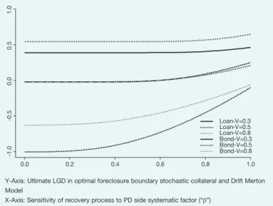
this parameter, that for higher correlation between firm asset value and recovery value return the LGD is higher and increases at a faster rate, and that for bonds these curves lie above and increase at a faster rate. In Figure 2 we show the ultimate LGD as a function of the volatility β in the recovery rate process attributable to the PD side systematic factor, fixing LGD side volatility υ = 0.5, for different firm values at default at Vt = (0.3,
0.5, 0.8). We observe that ultimate LGD increases at an increasing rate in this parameter, that for lower firm asset values the LGD is higher but increases at a slower rate, and that for bonds these curves lie above and increase at a lower rate.
Empirical analysis – calibration of models
In this section we describe our strategy for estimating parameters of the models for ultimate LGD by full-information maximum likelihood (FIML.) This involves a consideration of the LGD implied in the market at time of default tDi for the ith instrument in recovery segment s, denoted LGD
i,s,tiD.
This is the expected, discounted ultimate loss-given-default LGDi,s,tiE at
time of emergence tEi as given by any of our models m, LGDPs,m (θs,m)
over the resolution period tE i,s – tDi,s
(4.1)
Where θs,m is the parameter vector for segment s under model m,
ex-pectation is taken with respect to physical measure P, discounting is at risk adjusted rate appropriate to the instrument rDi,s and it is assumed that the time-to-resolution tE
i,s – tDi,s is known. In order to account for the
fact that we cannot observe expected recovery prices ex-ante, as only by coincidence would they coincide with expectations, we invoke market rationality to postulate that for a segment homogenous with respect to recovery risk the difference between expected and average realized re-coveries should be small. We formulate this by defining the normalized forecast error as:
(4.2)
This is the forecast error as a proportion of the LGD implied by the market at default (a ‘unit-free’ measure of recovery uncertainty) and the square root of the time-to-resolution. This is a mechanism to control for the likely increase in uncertainty with time-to-resolution, which effectively puts more weight on longer resolutions, increasing the estimate of the loss-severity. The idea behind this is that more information is revealed as the emergence point is approached, hence a decrease in risk. Alternatively, we can analyze εi,s≡ [LGDPs,m (θs,m) – LGDi,s,tiE] ÷ LGDi,s,tiD, the
fore-cast error that is non-time adjusted, and argue that its standard error
0.5 0.6 0.7 0.8 0.9 1.0 0. 00 .2 0. 40 .6 0. 81 .0 Loan-cor(R,V)=0.15 Loan-cor(R,V)=0.05 Loan-cor(R,V)=0.45 Bond-cor(R,V)=0.15 Bond-cor(R,V)=0.05 Bond-cor(R,V)=0.45 0.0 0.2 0.4 0.6 0.8 1.0 -1 .0 -0 .5 0. 00 .5 1. 0 Loan-V=0.3 Loan-V=0.5 Loan-V=0.8 Bond-V=0.3 Bond-V=0.5 Bond-V=0.8
Y-Axis: Ultimate LGD in optimal foreclosure boundary stochastic collateral and Drift Merton Model
X-Axis: Sensitivity of recovery process to LGD side systematic (“η”)
Figure 1 – Ultimate loss-give-default versus sensitivity of recovery process to LGD side systematic factor
0.5 0.6 0.7 0.8 0.9 1.0 0. 00 .2 0. 40 .6 0. 81 .0 Loan-cor(R,V)=0.15 Loan-cor(R,V)=0.05 Loan-cor(R,V)=0.45 Bond-cor(R,V)=0.15 Bond-cor(R,V)=0.05 Bond-cor(R,V)=0.45 0.0 0.2 0.4 0.6 0.8 1.0 -1 .0 -0 .5 0. 00 .5 1. 0 Loan-V=0.3 Loan-V=0.5 Loan-V=0.8 Bond-V=0.3 Bond-V=0.5 Bond-V=0.8
Y-Axis: Ultimate LGD in optimal foreclosure boundary stochastic collateral and Drift Merton Model
X-Axis: Sensitivity of recovery process to PD side systematic factor (“β”)
Figure 2 – Ultimate loss-given-default versus sensitivity of recovery process to PD side systematic factor
37 is proportional to (tE
i,s – tDi,s)1/2, which is consistent with an economy in
which information is revealed uniformly and independently through time [Miu and Ozdemir (2005)]. Assuming that the errors ε˜i,s in (4.2) are
stan-dard normal,8 we may use full-information maximum likelihood (FIML), by maximizing the log-likelihood (LL) function:
(4.3)
This turns out to be equivalent to minimizing the squared normalized forecast errors:
(4.4)
We may derive a measure of uncertainty of our estimate by the ML
8 If the errors are i.i.d and from symmetric distributions, then we can still obtain consistent estimates through ML, which has the interpretations as the quasi-ML estimator.
The Capco Institute Journal of Financial Transformation
Empirical Implementation of a 2-Factor Structural Model for Loss-Given-Default
Bankruptcy Out-of-court Total
Count Average
Standard error
of the mean Count Average
Standard error
of the mean Count Average
Standard error of the mean Bonds and term loans Return on defaulted debt1
1072 28.32% 3.47% 59 45.11% 19.57% 1131 29.19% 3.44% LGD at default2 55.97% 0.96% 38.98% 3.29% 55.08% 0.93% Discounted LGD3 51.43% 1.15% 33.89% 3.05% 50.52% 1.10% Time-to-resolution4 1.7263 0.0433 0.0665 0.0333 1.6398 0.0425 Principal at default5 207,581 9,043 416,751 65,675 218,493 9,323
Bonds Return on defaulted debt1
837 25.44% 3.75% 47 44.22% 21.90% 884 26.44% 3.74% LGD at default2 57.03% 1.97% 37.02% 5.40% 55.96% 1.88% Discounted LGD3 52.44% 1.30% 30.96% 3.00% 51.30% 1.25% Time-to-resolution4 1.8274 0.0486 0.0828 0.0415 1.7346 0.0424 Principal at default5 214,893 11,148 432,061 72,727 226,439 11,347
Revolvers Return on defaulted Debt1
250 26.93% 7.74% 17 10.32% 4.61% 267 25.88% 7.26% LGD at default2 54.37% 1.96% 33.35% 8.10% 53.03% 1.93% Discounted LGD3 52.03% 2.31% 33.33% 7.63% 50.84% 2.23% Time-to-resolution4 1.4089 0.0798 0.0027 0.0000 1.3194 0.0776 Principal at default5 205,028 19,378 246,163 78,208 207,647 18,786
Loans Return on defaulted Debt1
485 32.57% 5.71% 29 26.161% 18.872% 514 32.21% 5.49% LGD at default2 53.31% 9.90% 38.86% 7.22% 52.50% 3.21% Discounted LGD3 50.00% 1.68% 38.31% 5.79% 49.34% 2.25% Time-to-resolution4 1.3884 0.0605 0.0027 0.0000 1.3102 0.0816 Principal at default5 193,647 11,336 291,939 78,628 199,192 16,088
Total Return on defaulted debt1
1322 28.05% 3.17% 76 37.33% 15.29% 1398 28.56% 3.11% LGD at default2 55.66% 0.86% 37.72% 3.12% 54.69% 0.84% Discounted LGD3 51.55% 1.03% 33.76% 2.89% 50.58% 0.99% Time-to-resolution4 1.6663 0.0384 0.0522 0.0260 1.5786 0.0376 Principal at default5 207,099 8,194 378,593 54,302 216,422 8,351
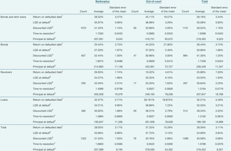
1 – Annualized return or yield on defaulted debt from the date of default (bankruptcy filing or distressed renegotiation date) to the date of resolution (settlement of renegotiation or emergence from Chapter 11).
2 – Par minus the price of defaulted debt at the time of default (average 30-45 days after default) as a percent of par.
3 – The ultimate dollar loss-given-default on the defaulted debt instrument = 1 – (total recovery at emergence from bankruptcy or time of final settlement)/(outstanding at default). Alternatively, this can be expressed as (outstanding at default – total ultimate loss)/(outstanding at default)
4 – The total instrument outstanding at default.
5 – The time in years from the instrument default date to the time of ultimate recovery.
Table 1 – Characteristics of loss-given-default and return on defaulted debt observations by default and instrument type (Moody’s Ultimate Recovery Database 1987-2009)
38
standard errors from the Hessian matrix evaluated at the optimum:
(4.5)
Data and estimation results
We summarize basic characteristics of our dataset in Table 1 and the maximum likelihood estimates are shown in Table 2. These are based upon our analysis of defaulted bonds and loans in the Moody’s Ultimate Recovery (MURD™) database release as of August, 2009. This contains the market values of defaulted instruments at or near the time of default9, as well as the values of such pre-petition instruments (or of instruments received in settlement) at the time of default resolution. This database is largely representative of the U.S. large-corporate loss experience, from
the mid 1980s to the present, including most of the major corporate bankruptcies occurring in this period. Table 1 shows summary statistics of various quantities of interest according to instrument type (bank loan, bond, term loan, or revolver) and default type (bankruptcy under Chapter 11 or out-of-court renegotiation). First, we annualized the return or yield on defaulted debt from the date of default (bankruptcy filing or distressed renegotiation date) to the date of resolution (settlement of renegotiation or emergence from Chapter 11), henceforth abbreviated as ‘RDD.’ Sec-ond, the trading price at default implied LGD (‘TLGD’), or par minus the trading price of defaulted debt at the time of default (average 30-45 days after default) as a percent of par value. Third, our measure of ultimate loss
Recovery segment Parameter s (1) μ (2) β (3) ν (4) s
R(5) pRβ(6) pRν(7) (βs)0.5 κa(8) a (9) ηa(10) ς (11) Seniority class Revolving credit / term loan Est. 4.32% 18.63% 18.16% 36.83% 41.06% 19.55% 80.45% 12.82% 3.96% 37.08% 48.85% 20.88% Std. Err. 0.5474% 0.9177% 0.7310% 1.3719% 0.4190% 0.0755% 4.2546% 3.2125% 0.9215% Senior secured bonds Est. 5.47% 16.99% 16.54% 30.41% 34.62% 22.83% 77.17% 11.64% 4.40% 33.66% 44.43% 18.99% Std. Err. 0.5314% 0.8613% 0.6008% 1.3104% 0.7448% 0.0602% 3.5085% 2.6903% 0.8297% Senior unsecured bonds Est. 6.82% 14.16% 13.82% 24.38% 28.02% 24.30% 75.70% 9.71% 5.50% 28.07% 37.04% 15.83% Std. Err. 0.5993% 1.0813% 1.3913% 1.9947% 0.6165% 0.0281% 2.887% 2.2441% 0.6504% Senior subordinated bonds Est. 8.19% 11.33% 12.02% 17.35% 21.11% 32.43% 67.57% 7.76% 4.42% 22.45% 29.68% 12.69% Std. Err. 0.6216% 1.0087% 1.0482% 1.0389% 0.9775% 0.0181% 2.0056% 2.0132% 1.0016% Subordinated bonds Est. 9.05% 9.60% 10.24% 12.37% 16.06% 40.66% 59.34% 5.97% 3.34% 18.80% 18.69% 9.43% Std. Err. 0.6192% 1.0721% 1.0128% 1.0771% 0.9142% 0.0106% 2.049% 2.0014% 1.0142%
Value log-likelihood function -371.09
Degrees of freedom 1391
P-value of likelihood ratio statistic 4.69E-03
In-sample
/time
diagnostic
statistics
Area under ROC curve 93.14%
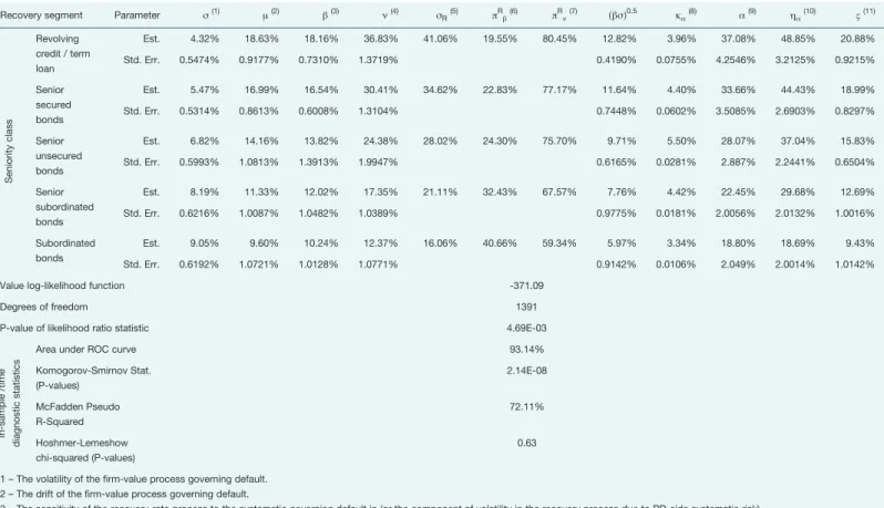
Komogorov-Smirnov Stat. (P-values) 2.14E-08 McFadden Pseudo R-Squared 72.11% Hoshmer-Lemeshow chi-squared (P-values) 0.63 1 – The volatility of the firm-value process governing default.
2 – The drift of the firm-value process governing default.
3 – The sensitivity of the recovery-rate process to the systematic governing default in (or the component of volatility in the recovery process due to PD-side systematic risk). 4 – The sensitivity of the recovery-rate process to the systematic governing collateral value (or the component of volatility in the recovery process due to LGD-side systematic risk). 5 – The total volatility of the recovery rate process: sqrt(β2+ν2)
6 – Component of total recovery variance attributable to PD-side (asset value) uncertainty: β2/(β2+ν2) 7 – Component of total recovery variance attributable to LGD-side (collateral value) uncertainty: ν2/(β2+ν2)
8 – The speed of the mean-reversion in the random drift in the recovery rate process. 9 – The long-run mean of the random drift in the recovery arte process.
10 – The volatility of the random drift in the recovery rate process.
11 – The correlation of the random processes in drift of and the level of the recovery rate process.
Table 2 – Full information maximum likelihood estimation of option theoretic two-factor structural model of ultimate loss-given-default with optimal foreclosure boundary, systematic recovery risk and random drift in the recovery process (Moody’s Ultimate Recovery Database 1987-2009)
9 This is an average of trading prices from 30 to 45 days following the default event. A set of dealers is polled every day and the minimum/maximum quote is thrown out. This is done by experts at Moody’s.
39 severity, the dollar loss-given-default on the debt instrument at
emer-gence from bankruptcy or time of final settlement (ULGD), computed as par minus either values of pre-petition or settlement instruments at reso-lution. We also summarize two additional variables in Table 1, the total instrument outstanding at default, and the time in years from the instru-ment default date to the time of ultimate recovery. The preponderance of this sample is made up of bankruptcies as opposed to out-of-court settlements, 1322 out of a total of 1398 instruments. We note that out-of-court settlements have lower LGDs by either the trading or ultimate measures, 37.7% and 33.8%, as compared to Chapter 11’s, 55.7% and 51.6%, respectively; and the heavy weight of bankruptcies are reflected in how close the latter are to the overall averages, 54.7% and 50.6% for TLGD and ULGD, respectively. Interestingly, not only do distressed renegotiations have lower loss severities, but such debt performs better over the default period than bankruptcies, RDD of 37.3% as compared to 28.1%, as compared to an overall RDD of 28.6%. We also note that the TLGD is higher than the ULGD by around 5% across default and instru-ment types, 55.7% (37.7%) as compared to 51.6% (33.8%) for bankrupt-cies (renegotiations). Finally, we find that loans have better recoveries by both measures as well higher returns on defaulted debt, respective average TLGD, ULGD and RDD are 52.5%, 49.35% and 32.2%. In Table 2 we present the full-information maximum likelihood estimation (FIML) results of the leading model for ultimate LGD derived in this paper, the two-factor structural model of ultimate loss-given-default, with sys-tematic recovery risk and random drift (2FSM-SR&RD) on the recovery.10 The model is estimated along with the optimal foreclosure boundary con-straint. We first discuss the MLE point estimates of the parameters gov-erning the firm value process and default risk, or the ‘PD-side.’ Regarding the parameter s, which is the volatility of the firm-value process govern-ing default, we observe that estimates are decreasgovern-ing in seniority class, ranging from 9.1% to 4.3% from subordinated bonds to senior loans, re-spectively. As standard errors range in 1% to 2%, increasing in seniority rank, these differences across seniority classes and models are generally statistically significant. Regarding the MLE point estimates of the param-eter μ, which is the drift of the firm-value process governing default, we observe estimates are increasing in seniority class, ranging from 9.6% to 18.6% from subordinated bonds to loans, respectively. These too are statistically significant across seniorities. The fact that we are observing different estimates of a single firm value process across seniorities is evi-dence that models which attribute identical default risk across different instrument types are mispecified – in fact, we are measuring lower default risk (i.e., lower asset value volatility and greater drift in firm-value) in loans and senior secured bonds as compared to unsecured and subordinated bonds. A key finding concerns the magnitudes and composition of the components of recovery volatility across maturities inferred from the model calibration. The MLE point estimates of the parameter β, the sen-sitivity of the recovery-rate process to the systematic factor governing
default (or due to PD-side systematic risk), increases in seniority class, from 10.2% for subordinated bonds to 18.2% for senior bank loans. On the other hand, estimates of the parameter υ, the sensitivity of the recov-ery-rate process to the systematic factor governing collateral value (or due to LGD-side systematic risk), are greater than β across seniorities, and similarly increases from 12.4% for subordinated bonds to 36.8% for bank loans. This monotonic increase in both β and υ as we move up in the hierarchy of the capital structure from lower to higher ranked instru-ments has the interpretation of a greater sensitivity in the recovery rate process attributable to both systematic risks, implying that total recovery volatility sR = (β2 + υ2)1/2 increases from higher to lower ELGD
instru-ments, from 16.1% for subordinated bonds to 41.1% for senior loans. However, we see that the proportion of the total recovery volatility at-tributable to systematic risk in collateral (firm) value, or the LGD (PD) side, is increasing (decreasing) in seniority from 59.3% to 80.5% (40.7% to 19.6%) from subordinated bonds to senior bank loans. Consequently, more senior instruments not only exhibit greater recovery volatility than less senior instruments, but a larger component of this volatility is driven by the collateral rather than the asset value process.
The next set of results concern the random drift in the recovery rate pro-cess. The MLE point estimates of the parameter κa, the speed of the
mean-reversion, is hump-shape in seniority class, ranging from 3.3% subordinated bonds, to 5.5% for senior unsecured bonds, to 4.0% for loans, respectively. Estimates of the parameter a, the long-run mean of the random drift in the recovery rate process, increases in seniority class from 18.8% for subordinated bonds to 37.1% for senior bank loans. This monotonic increase in a from lower to higher ranked instruments has the interpretation of greater expected return of the recovery rate process in-ferred from lower ELGD (or greater expected recovery) instruments as we move up in the hierarchy of the capital structure. We see that the volatility of the random drift in the recovery rate process ηa, increases in seniority
class, ranging from 18.7% for subordinated bonds to 48.9% for senior loans. The monotonic increase in ηa as we move from lower to higher
ranked instruments has the interpretation of greater volatility in expected return of the recovery rate process inferred from lower ELGD (or greater expected recovery) instruments as we move up in the hierarchy of the capital structure. Finally, estimates of the parameter ζ, the correlation of the random processes in drift of and the level of the recovery rate process, increase in seniority class from 9.4% for subordinated bonds to 20.9% for senior bank loans. Finally with respect to parameter esti-mates, regarding the MLE point estimates of the correlation between the default and recovery rate processes , we observe that estimates are increasing in seniority class, ranging from 6.0% for subordinated bonds to 12.8% for senior loans.
The Capco Institute Journal of Financial Transformation
Empirical Implementation of a 2-Factor Structural Model for Loss-Given-Default
10 Estimates for the baseline Merton structural model (BMSM) and for the Merton structural model with stochastic drift (MSM-SD) are available upon request.
40
We conclude this section by discussing the quality of the estimates and model performance measures. Across seniority classes, parameter timates are all statistically significant, and the magnitudes of such es-timates are in general distinguishable across segments at conventional significance levels. The likelihood ratio statistic indicates that we can reject the null hypothesis that all parameter estimates are equal to zero across all ELGD segments, a p-value of 4.7e-3. We also show various di-agnostics that assess in-sample fit, which show that the model performs well-in sample. The area under receiver operating characteristic curve (AUROC) of 93.1% is high by commonly accepted standards, indicat-ing a good ability of the model to discriminate between high and low LGD defaulted instruments. Another test of discriminatory ability of the models is the Kolmogorov-Smirnov (KS) statistic, the very small p-value 2.1e-8 indicating adequate separation in the distributions of the low and high LGD instruments in the model.11 We also show 2 tests of predictive accuracy, which is the ability of the model to accurately quantify a level of LGD. The McFadden psuedo r-squared (MPR2) is high by commonly accepted standards, 72.1%, indicating a high rank-order correlation be-tween model and realized LGDs of defaulted instruments. Another test of predictive accuracy of the models is the Hoshmer-Lemeshow (HL) statistic, high p-values of 0.63 indicating high accuracy of the model to forecast cardinal LGD.
Downturn LGD
In this section we explore the implications of our model with respect to downturn LGD. This is a critical component of the quantification process in Basel II advanced IRB framework for regulatory capital. The Final Rule (FR) in the U.S. [OCC et al. (2007)] requires banks that either wish, or are required, to qualify for treatment under the advanced approach to estimate a downturn LGD. We paraphrase the FR, this is an LGD esti-mated during an historical reference period during which default rates are elevated within an institution’s loan portfolio. In Figures 3 we plot the ratios of the downturn LGD to the expected LGD. This is derived by conditioning on the 99.9th quantile of the PD side systematic factor in the model for ultimate LGD. We show this for loans and bonds, as well as for different settings of key parameters ( , υ, or ηa) in the plot, with other
parameters set to the MLE estimates. We observe that the LGD mark-up for downturn is montonically declining in ELGD, which is indicative of lower tail risk in recovery for lower ELGD instruments. It is also greater than unity in all cases, and approaches 1 as ELGD approaches 1. This multiple is higher for bonds than for loans, as well as for either higher PD-LGD correlation or collateral specific volatility υ, although these differences narrow for higher ELGD.
Model validation
In this final section we validate our model, in particular, we implement an out-of-sample and out-of-time analysis, on a rolling annual cohort basis for the final 12 years of our sample. Furthermore, we augment
this by resampling on both the training and prediction samples, a non-parametric bootstrap [Efron (1979), Efron and Tibshirani (1986), Davison and Hinkley (1997)]. The procedure is as follows: the first training (or es-timation) sample is established as the cohorts defaulting in the 10 years 1987-1996, and the first prediction (or validation) sample is established as the 1997 cohort. Then we resample 100,000 times with replacement from the training sample the 1987-1996 cohorts and for the prediction sample 1997 cohort, and then based upon the fitted model in the former we evaluate the model based upon the latter. We then augment the train-ing sample with the 1997 cohort, and establish the 1998 cohort as the prediction sample, and repeat this. This is continued until we have left the 2008 cohort as the holdout. Finally, to form our final holdout sample, we pool all of our out-of-sample resampled prediction cohorts, the 12 years running from 1997 to 2008. We then analyze the distributional properties (such as median, dispersion, and shape) of the two key diagnostic sta-tistics: the Spearman rank-order correlation for discriminatory (or clas-sification) accuracy, and the Hoshmer-Lemeshow chi-squared P-values for predictive accuracy, or calibration.
Before discussing the results, we briefly describe the two alternative frameworks for predicting ultimate LGD that are to be compared to the 2-factor structural model with systematic recovery and random drift (2FSM-SR&RD) developed in this paper. First, we implement a full-in-formation maximum likelihood simultaneous equation regression model (FIMLE-SERM) for ultimate LGD, which is an econometric model built
0.0 0.2 0.4 0.6 0.8 1.0 1 2 3 4 5 Loans/corr(R,V)=0.1 Bonds/corr(R,V)=0.1 Loans/cor(R,V)=0.05 Bonds/cor(R,V)=0.05 Loans/stdev(R|V)==0.3 Bonds/stdev(R|V)==0.2 Loans/stdev(R|V)==0.3 Bonds/stdev(R|V)==0.2 Y-Axis: DLGD/ELGD X-Axis: ELGD
Figure 3 – Ratio of ultimate downturn to expected LGD versus ELGD at 99.9th percentile of PD-side systematic factor Z
11 In these tests we take the median LGD to be the cut-off that distinguishes between a high and low realized LGD.
41
The Capco Institute Journal of Financial Transformation
Empirical Implementation of a 2-Factor Structural Model for Loss-Given-Default
upon observations in MURD at both the instrument and obligor level. FIMLE is used to model the endogeneity of the relationship between LGD at the firm and instrument levels in an internally consistent manner. This technique enables us to build a model that can help us understand some of the structural determinants of LGD, and potentially improve our fore-casts of LGD. This model contains 199 observations from the MURD™ with variables: long term debt to market value of equity, book value of as-sets quantile, intangibles to book value of asas-sets, interest coverage ratio, free cash flow to book value of assets, net income to net sales, number of major creditor classes, percentage of secured debt, Altman Z-Score, debt vintage (time since issued), Moody’s 12 month trailing speculative grade default rate, industry dummy, filing district dummy, and a pre-packaged bankruptcy dummy. Detailed discussion of the results can be found in Jacobs and Karagozoglu (2010). The second alternative model we consider addresses the problem of non-parametrically estimating a regression relationship, in which there are several independent variables and in which the dependent variable is bounded, as an application to the distribution of LGD. Standard non-parametric estimators of unknown probability distribution functions, whether conditional or not, utilize the Gaussian kernel [Silverman (1982), Hardle and Linton (1994), and Pagan
and Ullah (1999)]. It is well known that there exists a boundary bias with a Gaussian kernel, which assigns non-zero density outside the support on the dependent variable, when smoothing near the boundary. Chen (1999) has proposed a beta kernel density estimator (BKDE) defined on the unit interval [0,1], having the appealing properties of flexible functional form, a bounded support, simplicity of estimation, non-negativity, and an optimal rate of convergence n-4/5 in finite samples. Furthermore, even if the true
density is unbounded at the boundaries, the BKDE remains consistent [Bouezmarni and Rolin (2001)], which is important in the context of LGD, as there are point masses (observation clustered at 0% and 100%) in empirical applications. Detailed derivation of this model can be found in Jacobs and Karagozoglu (2010). We extend the BKDE [Renault and Scalliet (2004)] to a generalized beta kernel conditional density estimator (GBKDE), in which the density is a function of several independent vari-ables, which affect the smoothing through the dependency of the beta distribution parameters upon these variables.
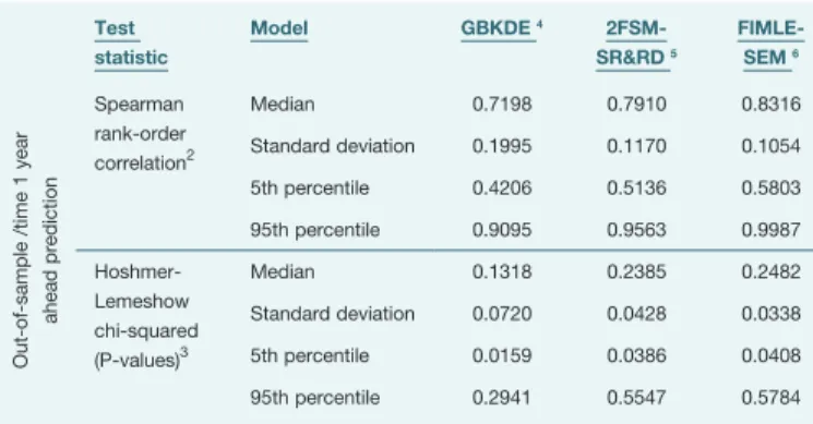
Results of the model validation are shown in Table 3. We see that while all models perform decently out–of-sample in terms of rank ordering capa-bility, FIMLE-SEM performs the best (median = 83.2%), the GBKDE the worst (median = 72.0%), and our 2FSM-SR&RD in the middle (median = 79.1%). It is also evident from the Table and figures that the better per-forming models are also less dispersed and exhibit less multi-modality. However, the structural model is closer in performance to the regression model by the distribution of the Pearson correlation, and indeed there is a lot of overlap in these. Unfortunately, the out-of-sample predictive accuracy is not as encouraging for any of the models, as in a sizable proportion of the runs we can reject adequacy of fit (i.e., p-values indi-cating rejection of the null of model it at conventional levels). The rank ordering of model performance for Hoshmer-Lemeshow p-values of test statistics is the same as for the Pearson statistics: FIMLE-SEM performs the best (median = 24.8%), the GBKDE the worst (median = 13.2%), and our 2FSM-SR&RD in the middle (median = 23.9%); and the structural model developed herein is comparable in out-of-sample predictive ac-curacy to the high-dimensional regression model. We conclude that while all models are challenged in predicting cardinal levels of ultimate LGD out-of-sample, it is remarkable that a relatively parsimonious structural model of ultimate LGD can perform so closely to a highly parameterized econometric model.
Conclusions and directions for future research
In this study we have developed a theoretical model for ultimate loss-giv-en-default, having many intuitive and realistic features, in the structural credit risk modeling framework. Our extension admits differential senior-ity within the capital structure, an independent process representing a source of undiversifiable recovery risk with a stochastic drift, and an op-timal foreclosure threshold. We also analyzed the comparative statics of this model. In the empirical analysis we calibrated the model for ultimate
Test statistic Model GBKDE 4 2FSM-SR&RD 5 FIMLE-SEM 6 Out-of-sample /time 1 year ahead prediction Spearman rank-order correlation2 Median 0.7198 0.7910 0.8316 Standard deviation 0.1995 0.1170 0.1054 5th percentile 0.4206 0.5136 0.5803 95th percentile 0.9095 0.9563 0.9987 Hoshmer-Lemeshow chi-squared (P-values)3 Median 0.1318 0.2385 0.2482 Standard deviation 0.0720 0.0428 0.0338 5th percentile 0.0159 0.0386 0.0408 95th percentile 0.2941 0.5547 0.5784 1 – In each run, observations are sampled randomly with replacement from the training and
prediction samples, the model is estimated in the training sample and observations are classified in the prediction period, and this is repeated 100,000 times.
2 – The correlation between the ranks of the predicted and realizations, a measure of the discriminatory accuracy of the model.
3 – A normalized average deviation between empirical frequencies and average modeled probabilities across deciles of risk, ranked according to modeled probabilities, a measure of model fit or predictive accuracy of the model.
4 – Generalized beta kernel conditional density estimator model.
5 – Two factor structural Merton systematic recovery and random drift model. 6 – Full-information maximum likelihood simultaneous equation regression model. 199
observations with variables: long term debt to market value of equity, book value of assets quantile, intangibles to book value of assets, interest coverage ratio, free cash flow to book value of assets, net income to net sales, number of major creditor classes, percent secured debt, Altman Z-Score, debt vintage (time since issued), Moody’s 12 month trailing speculative grade default rate, industry dummy, filing district dummy and prepackaged bankruptcy dummy.
Table 3 – Bootstrapped1 out-of-sample and out-of-time classification and
predictive accuracy model comparison analysis of alternative models for ultimate loss-given-default (Moody’s Ultimate Recovery Database 1987-2009)
42
LGD on bonds and loans, having both trading prices at default and at res-olution of default, utilizing an extensive sample of agency rated defaulted firms in the Moody’s URD™. These 800 defaults are largely representative of the U.S. large corporate loss experience, for which we have the com-plete capital structures, and can track the recoveries on all instruments to the time of default to the time of resolution. We demonstrated that parameter estimates vary significantly across recovery segments, finding that the estimated volatilities of the recovery rate processes and their random drifts are increasing in seniority; in particular, for 1st lien bank loans as compared to senior secured or unsecured bonds. Furthermore, we found that the proportion of recovery volatility attributable to the LGD-side (as opposed to the PD-LGD-side) systematic factors to be higher for more senior instruments. We argued that this reflects the inherently greater risk in the ultimate recovery for higher ranked instruments having lower ex-pected loss severities. In an exercise highly relevant to requirements for the quantification of a downturn LGD for advanced IRB under Basel II, we analyzed the implications of our model for this purpose, finding the later to be declining for higher expected LGD, higher for lower ranked instru-ments, and increasing in the correlation between the process driving firm default and recovery on collateral. Finally, we validated our model in an out-of-sample bootstrapping exercise, comparing it to two alternatives, a high-dimensional regression model and a non-parametric benchmark, both based upon the same MURD data. We found our model to compare favorably in this exercise. We conclude that our model is worthy of con-sideration to risk managers, as well as supervisors concerned with ad-vanced IRB under the Basel II capital accord. It can be a valuable bench-mark for internally developed models for ultimate LGD, as this model can be calibrated to LGD observed at default (either market prices or model forecasts, if defaulted instruments are non-marketable) and to ultimate LGD measured from workout recoveries. Finally, risk managers can use our model as an input into internal credit capital models.
References
• Acharya, V. V., S. T. Bharath, and A. Srinivasan, 2007, “Does industry-wide distress affect defaulted firms? Evidence from creditor recoveries,” Journal of Political Economy, 85:3, 787-821
• Altman, E. I., 1968, “Financial ratios, discriminant analysis and the prediction of corporate bankruptcy,” Journal of Finance, 23, 589-609
• Altman, E. I., 2006, “Default recovery rates and LGD in credit risk modeling and practice: an updated review of the literature and empirical evidence,” Working paper, NYU Salomon Center, November
• Altman, E. I., R. Haldeman, and P. Narayanan, 1977, “Zetaä analysis: a new model to predict corporate bankruptcies,” Journal of Banking and Finance, 1:1, 29-54
• Altman, E. I., and A. Eberhart, 1994, “Do seniority provision protect bondholders’ investments?” Journal of Portfolio Management, Summer, 67-75
• Altman, E. I., and V. M. Kishore, 1996, “Almost everything you wanted to know about recoveries on defaulted bonds. Financial Analysts Journal, Nov/Dec, 56-62
• Altman, E. I., A. Resti, and A. Sironi, 2001, “Analyzing and explaining default recovery rates,” ISDA Research Report, London, December
• Altman, E. I., A. Resti, and A. Sironi, 2003, “Default recovery rates in credit risk modeling: a review of the literature and empirical evidence,” Working paper, New York University Salomon Center, February
• Altman, E. I., B. Brady, A. Resti, and A. Sironi, 2005, “The link between default and recovery rates: theory, empirical evidence and implications,” Journa1 of Business 78, 2203-2228
• Araten, M., M. Jacobs, Jr., and P. Varshney, 2004, “Measuring loss given default on commercial loans for the JP Morgan Chase wholesale bank: an 18 year internal study,” RMA Journal, 86, 96-103
• Asarnow, E., and D. Edwards, 1995, “Measuring loss on defaulted bank loans: a 24-year study, Journal of Commercial Lending,” 77:7, 11-23
• Bakshi, G., D. Madan, and F. Zhang, 2001, “Understanding the role of recovery in default risk models: empirical comparisons and implied recovery rates,” Federal Reserve Board, Finance and Economics Discussion Series #37
• Basel Committee on Banking Supervision, 2003, The new Basel accord, Consultative Document, Bank for International Settlements (BIS), April
• Basel Committee on Banking Supervision, 2005, Guidance on paragraph 468 of the framework document, BIS, July
• Basel Committee on Banking Supervision, 2006, International convergence on capital measurement and capital standards: a revised framework. BIS, June
• Bjerksund, P., 1991, “Contingent claims evaluation when the convenience yield is stochastic: analytical results,” working paper, Norwegian School of Economics and Business Administration
• Black, F., and J. C. Cox, 1976, “Valuing corporate securities: some effects of bond indenture provisions,” Journal of Finance, 31, 637-659
• Bouezmarni, T., and J. M. Rolin, 2001, “Consistency of beta kernel density function estimator,” Canadian Journal of Statistics, 31, 89-98
• Chen, S. X., 1999, “Beta kernel estimators for density functions,” Computational Statistics & Data Analysis, 31, 131-145
• Carey, M., and M. Gordy, 2007, “The bank as grim reaper: debt decomposition and recoveries on defaulted debt,” Working paper, Federal Reserve Board
• Credit Suisse Financial Products, 1997, “Creditrisk+ – a credit risk management framework,” Technical Document
• Davison, A. C., and D. V. Hinkley, 1997, “Bootstrap methods and their application,” Cambridge University Press, Cambridge
• Dev, A., and M. Pykhtin, 2002, “Analytical approach to credit risk modeling,” Risk, March, S26–S32
• Duffie, D., 1998, “Defaultable term structure models with fractional recovery of par,” Working paper, Graduate School of Business, Stanford University
• Duffie, D., and K. J. Singleton, 1999, “Modeling the term structures of defaultable bonds,” Review of Financial Studies, 12, 687-720
• Duffie, D., and D. Lando, 2001, “Term structure of credit spreads with incomplete accounting information,” Econometrica, 69, 633-664
• Efron, B., 1979, “Bootstrap methods: another look at the jackknife,” American Statistician, 7, 1-23
• Duffie, D., and R. Tibshirani, 1986, “Bootstrap methods for standard errors, confidence intervals, and other measures of statistical accuracy,” Statistical Science 1, 54-75
• Finger, C., 1999, “Conditional approaches for CreditMetrics™ portfolio distributions,” CreditMetrics™ Monitor, April
• Franks, J., and W. Torous, 1989, “An empirical investigation of U.S. firms in reorganization,” Journal of Finance, 44, 747-769