Skip-GANomaly : skip connected and adversarially trained encoder-decoder anomaly detection.

Skip-GANomaly: Skip Connected and Adversarially

Trained Encoder-Decoder Anomaly Detection

Samet Akçay, Amir Atapour-Abarghouei, Toby P. Breckon

Abstract—Despite inherent ill-definition, anomaly detection is a research endeavour of great interest within machine learning and visual scene understanding alike. Most commonly, anomaly detection is considered as the detection of outliers within a given data distribution based on some measure of normality. The most significant challenge in real-world anomaly detection problems is that available data is highly imbalanced towards normality (i.e. non-anomalous) and contains at most a sub-set of all possible anomalous samples - hence limiting the use of well-established supervised learning methods. By contrast, we introduce an unsupervised anomaly detection model, trained only on the normal (non-anomalous, plentiful) samples in order to learn the normality distribution of the domain, and hence detect abnormality based on deviation from this model. Our proposed approach employs an encoder-decoder convolutional neural net-work with skip connections to thoroughly capture the multi-scale distribution of the normal data distribution in image space. Furthermore, utilizing an adversarial training scheme for this chosen architecture provides superior reconstruction both within image space and a lower-dimensional embedding vector space encoding. Minimizing the reconstruction error metric within both the image and hidden vector spaces during training aids the model to learn the distribution of normality as required. Higher reconstruction metrics during subsequent test and deployment are thus indicative of a deviation from this normal distribution, hence indicative of an anomaly. Experimentation over estab-lished anomaly detection benchmarks and challenging real-world datasets, within the context of X-ray security screening, shows the unique promise of such a proposed approach.

Index Terms—Anomaly Detection; Generative Adversar-ial Networks; Skip Connections; X-ray Security Screening, GANomaly

I. INTRODUCTION

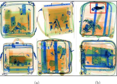
Anomaly detection is an increasingly important area within visual image understanding. Following recent trends in the field, there has been a significant increase in the availability of large datasets. However, in most cases such data re-sources are highly imbalanced towards examples of normality (non-anomalous), whilst lacking in examples of abnormality (anomalous) and offering only partial coverage of all possibil-ities which could encompass this latter class. This variation, and the somewhat unknown nature, of the anomalous class mean such datasets lack the capacity and diversity to train tra-ditional supervised detection approaches. In many application scenarios, such as the X-ray screening example illustrated in Figure 1, the availability of anomalous cases may be limited and may evolve over time due to external factors. Within such scenarios, unsupervised anomaly detection has become instrumental in modeling such data distributions, whereby the

(a) (b)

Fig. 1: Sub-sample of the X-ray screening application dataset used to train the proposed approach: (a) training data contains normal samples only, while the test data (b) comprises both normal and abnormal samples.

model is trained only on normal (non-anomalous) samples to capture the distribution of normality, and then evaluated on both unseen normal and abnormal (anomalous) examples to find their deviation from the distribution.

A significant body of prior work exists within anomaly detection for visual scene understanding [1]–[5] with a wide range of application domains [6]–[10]. A common hypoth-esis in such anomaly detection approaches is that abnormal samples differ from normality in not only image space but also with lower-dimensional latent space encoding. Hence, mapping images to lower-dimensional latent space becomes essential. The critical issue here is that capturing the distri-bution of the normal samples is rather challenging. Recent developments in Generative Adversarial Networks (GAN) [11], shown to be highly capable of obtaining input data distribution, have led to a renewed interest in the anomaly detection problem. Several contemporary studies demonstrate that the use of GAN has great promise to address this anomaly detection problem since they are inherently adept at mapping high-dimensional to lower-dimensional latent encoding and vice-versawith minimal information loss [9], [12], [13].

Schlegl et al. [9] trains a pre-trained GAN backwardly to map from image space to lower-dimensional latent space, hypothesizing that differences in latent space would yield

anomalies. Zenatiet al.[12] jointly train a two-network model to capture normal distribution by mapping from image space to latent space, and vice-versa. Akçay et al. [13] train an encoder-decoder-encoder network with the adversarial scheme to capture the normal distribution within the image and latent space. Sabokrou et al. [14] also train an adversarial network to capture the normal distribution, hypothesizing that the model would fail to generate abnormal samples, where the difference between the original and generated images would yield the abnormality. This prior work in the field [9], [12]– [14], empirically illustrates both the importance and promise of anomaly detection within dual image and latent space.

Here we propose a new method for anomaly detection via adversarial training over a skip-connected encoder-decoder (convolutional neural) network architecture. Whilst adversarial training has shown the promise of GAN in this domain [13], skip-connections within such UNet-style (encoder-decoder) [15] generator networks are known to enable the multi-scale capture of image space detail with sufficient capacity to gen-erate high-quality normal images drawn from the distribution the model has learned. Similar to [9], [12], [13], the proposed approach also seeks to learn the normal distribution in both the image and latent spaces via a GAN generator-discriminator paradigm. The discriminator network not only forces the generator to learn an improved model of the distribution but also works as a feature extractor such that it learns the recon-struction of the normal distribution within a lower-dimensional latent space. Evaluation of the model on various established benchmarks [16], [17] statistically illustrates superior anomaly detection task performance over prior work [9], [12], [13]. Subsequently, the main contributions of this paper are as follows:

• unsupervised anomaly detection — a unique unsu-pervised adversarial training regime, over a skip-connected encoder-decoder convolutional network archi-tecture, which yields superior reconstruction within the image and latent vector spaces.

• efficacy — an efficient anomaly detection algorithm achieving quantitatively and qualitatively superior perfor-mance against prior state-of-the-art approaches.

• reproducibility — a simple yet effective algorithmic ap-proach that can be readily reproduced.

II. RELATEDWORK

Anomaly detection is a major area of interest within the field of machine learning with various real-world applications spanning from biomedical [9] to video surveillance [10]. Recently, the existing literature within the field has grown considerably, leading to a proliferation of taxonomy papers [1]–[5]. Due to the current trends, the review in the paper primarily focuses on reconstruction-based anomaly detection approaches.

One of the most influential accounts of anomaly detection using adversarial training comes from Schlegl et al. [9]. The authors hypothesize that the latent vector of the GAN represents the distribution of the data. However, mapping to

the vector space of the GAN is not straightforward. To achieve this, the authors first train a generator and discriminator using only normal images. In the next stage, they utilize the pre-trained generator and discriminator by freezing the weights and remap to the latent vector by optimizing the GAN based on thez vector. During inference, the model pinpoints an anomaly by outputting a high anomaly score, resulting in significant improvements over previous work. The main limitation of this work is its computational complexity since the model employs a two-stage approach, and remapping the latent vector is extremely expensive. In a follow-up study, Zenati et al. [12] investigate the use of BiGAN [18] in an anomaly detection task, examining joint training to map from image space to latent space simultaneously, and vice-versa. Training the model via [9] yields superior results on the MNIST [19] dataset. In a similar study, in which image and latent vector spaces are optimized for anomaly detection, Akçayet al.[13] propose an adversarial network such that the generator comprises encoder-decoder-encoder sub-networks. The objective of the model is not only to minimize the distance between the real and fake normal images, but also minimize the distance within their latent vector representations jointly. The proposed approach achieves state-of-the-art performance both statistically and computationally.

Taken together, these studies support the notion that the use of reconstruction-based approaches shows promise within the field [9], [10], [12]–[14]. Motivated by the previous methods in which latent vectors are optimized [9], [12], [13], we propose an anomaly detection approach that utilizes an adversarially trained encoder-decoder with skip connections. The proposed approach learns representations within both image and latent vector space jointly and achieves numerically superior perfor-mance.

III. PROPOSEDAPPROACH

Before proceeding to explain our proposed approach, it is important to introduce the fundamental concepts.

A. Background

1) Generative Adversarial Networks (GAN): GAN are un-supervised deep neural architectures that learn to capture any input data distribution by predicting features from an initially hidden representation. Initially proposed in [11], the theory behind GAN is based on a competition between two networks within a zero-sum game framework, as initially used in game theory. The task of the first network, called Generator (G) is to capture the distribution of the input dataset for a given class label, by predicting features (or images) from a hidden repre-sentation, which is commonly a random noise vector. Hence, the generator network has a decoder network architecture such that it up-samples the input arbitrary latent representation to generate low-dimensional features. The task of the second network, called Discriminator (D), on the other hand, is to predict the correct class (i.e.,real vs. fake) based on the given features (or images). The discriminator network usually adopts an encoder network architecture such that for a given feature

map, it predicts its class label. With optimization based on a zero-sum game framework, each network strengthens its prediction capability until they reach an equilibrium.

Due to their inherent potential for capturing data distribu-tions, there is a growing body of literature that recognizes the importance of GAN [20]. Training two networks jointly to reach an equilibrium, however, is not a straightforward procedure, causing training instability issues. Recently, there has been a surge of interest in addressing the instability issues via several empirical methodologies [21], [22]. An innovative and seminal work of Radford and Chintala [23] pioneered a new approach to stabilize GAN training by using fully-convolutional layers and batch normalization [24] throughout the network. Another well-known attempt to stabilize GAN training is the use of Wasserstein loss in the training objective, which significantly improves training stability [25], [26].

2) Adversarial Auto-Encoders (AAE): Conceptually similar to GAN, AAE consist of a generator and a discriminator network. The generator follows a bow-tie architectural network style comprising both an encoder and a decoder. The task of the generator is to reconstruct the input data by down-sampling it into a latent representation first, and then by up-sampling the latent vector into the reconstructed data (image). The task of the discriminator network, which receives a latent vector as its input, is to predict whether this input is the latent vector from the auto-encoder or the prior distribution initialized arbitrarily. Training AAE provides superior reconstruction as well as the capability of controlling the latent space [20], [27], [28].

3) Inference within GAN: A strong correlation has been demonstrated between the manipulation of the input noise vector and the output of the generator network [23], [29]. Similar latent space variables have demonstrably produced visually similar high-resolution images [30]. One approach to finding the optimal latent vectors is to create similar images is to inversely map images back to their hidden space via their gradients [31]. Alternatively, with an additional encoder network that down-samples images into lower-dimensional latent space, vanilla GAN are reported to be capable of learning inverse mapping [18]. Another way to learn inference via inverse mapping is to jointly train two networks such that the former maps images to latent space, while the latter maps this latent space representation back into image space [32]. Based on these previous findings, the primary aim of this paper is to explore inference within GAN by exploiting the latent vector representation in order to find a unique representation for a normal (non anomalous) data distribution such that it can be statistically differentiated from unseen, unknown and varying abnormal (anomalous) data samples.

B. Proposed Approach

1) Problem Definition: This work proposes an unsuper-vised approach for anomaly detection.

We adversarially train our proposed convolutional network architecture in an unsupervised manner such that the concep-tual model is trained on normal samples only, and yet tested

Skip Con.

Loss Flow Input

Output Discr.Net

Conv FeatMap ConvTrans FeatMap Bottleneck Features

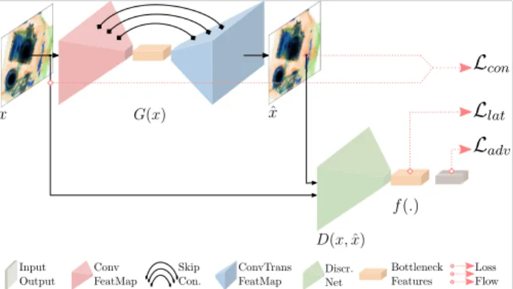
Fig. 2: Overview of the proposed adversarial training procedure.

on both normal and abnormal ones. Mathematically, we define and formulate our problem as the following:

An input dataset D is split into train Dtrn and test sets

Dtst such that Dtrn = {(x1, y1),(x2, y2), . . . ,(xm, ym)}

containsmnormal samples, whereyi= 0denotes the normal

class. The test set Dtst = {(x1, y1),(x2, y2), ...,(xm, ym)}

comprisesnnormal and abnormal samples, where yi∈[0,1]

for normal and abnormal classes, respectively. In practical settings, mn.

Based on the dataset defined above, we train our model f on Dtrn and evaluate its performance on Dtst. The training

objective (J) of the model f is to capture the distribution of Dtrn within not only image space but also hidden latent

vector space. Capturing the distribution within both dimen-sions by minimizing J enables the network to learn higher and lower level features that are unique to normal images. We hypothesize that defining an anomaly scoreA(.)based on the training objectiveJ would yield minimal anomaly scores for training samples —normal samples, but greater scores for abnormal images. Hence a higher anomaly score A(x) for a given sample x would indicate whether x is normal or abnormal with respect to the distribution of normal data learned byf fromDtrn during training.

2) Pipeline: Figure 2 shows a high-level overview of the proposed approach, which comprises a generator (G) and a discriminator (D) network, respectively. The networkGadopts a bow-tie architecture using an encoder (GE) and a decoder

(GD) network. The encoder network captures the distribution

of the input data by mapping the image (x) into lower-dimensional latent representation (z) such that GE : x→z,

where x∈Rw×h×c and z ∈ Rd. As illustrated in Figure 3,

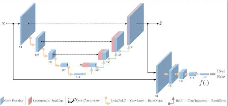
the networkGE reads input xthrough five blocks containing

Convolutional and BatchNorm layers as well as LeakyReLU activation function and outputs the latent representation z, which is also known as the bottleneck features that carries a unique representation of the input.

Being symmetrical to GE, the decoder network GD

up-samples the latent vectorzback to the input image dimension and reconstructs the output, denoted as xˆ. Motivated by [15], the decoder GD adopts skip-connection approach such

64 128 256 512 512 64 128 256 512 _Real Fake

Conv FeatMap Concatenated FeatMap Copy-Concatenate LeakyReLU + ConvLayer + BatchNorm ReLU + ConvTranspose + BatchNorm

64 128

256 512 100

Fig. 3: Details of the proposed network architecture.

concatenated to its corresponding up-sampling decoder layer (Figure 3). This use of skip connections provides substantial advantages via direct information transfer between the layers, preserving both local and global (multi-scale) information, and hence yielding better reconstruction.

The second network within the pipeline, shown in Figure 3 (b), called discriminator (D), predicts the class label of the given input. In this context, its task is to classify real images (x) from the fake ones (ˆx), generated by the network G. The network architecture of the discriminatorDfollows the same structure as the discriminator of the DCGAN approach presented in [23]. Besides being a classifier, the network D is also used as a feature extractor such that latent represen-tations of the input image x and the reconstructed image xˆ are computed. Extracting the features from the discriminator to perform inference within the latent space is one of the novel contributions of the proposed approach compared to the previous approaches [9], [12], [13].

Based on this multi-network architecture, explained above and shown in Figure3, the next section describes the proposed training objective and inference scheme.

C. Training Objective

As explained in Section III-B1, the idea proposed in this work is to train the model only on normal samples, and test on both normal and abnormal ones. The motivation is that we expect the model to be able to correctly reconstruct the normal samples either in image or latent vector space. The hypothesis is that the network is conversely expected to fail to reconstruct the abnormal samples as it is never trained on such abnormal examples. Hence, for abnormal samples, one would expect a higher loss for the reconstruction of the output image xˆ or the latent representation zˆ. To validate this, we propose to

combine three loss values (Adversarial, Contextual, Latent), each of which has its own contribution to make within the overall training objective.

1) Adversarial Loss: In order to maximize the reconstruc-tion capability for the normal images x during training, we utilize the adversarial loss proposed in [11]. This loss, shown in Equation 1, ensures that the network G reconstructs a normal image x to xˆ as realistically as possible, while the discriminator network D classifies the real and the (fake) generated samples. The task here is to minimize this objective for G, and maximize for D to achieve min

G maxD Ladv, where

Ladv is denoted as Ladv=_xE ∼px [logD(x)] + _E x∼px [log(1−D(ˆx)]. (1) 2) Contextual Loss: The adversarial loss defined in Section III-C1 forces the model to generate realistic samples, but does not guarantee to learn contextual information regarding the input. To explicitly learn this contextual information to sufficiently capture the input data distribution for the normal samples, we apply an L1 loss between the input x and the reconstructed output xˆ. This loss component ensures that the model is capable of generating contextually similar images to normal samples. The contextual loss of the training objective is shown below:

Lcon= E

x∼px

||x−xˆ||1. (2) 3) Latent Loss: With the adversarial and contextual losses defined above, the model is able to generate realistic and contextually similar images. In addition to these objectives, we aim to reconstruct latent representations for the input x and the generated normal samples xˆ as similar as possible. This

is to ensure that the network is capable of producing contex-tually sound latent representations for common examples. As depicted in Figure 3(b), we use the final convolutional layer of the discriminator D, and extract the features of xandxˆto reconstruct their latent representations such thatz=f(x)and ˆ

z=f(ˆx). The latent representation loss therefore becomes:

Llat= E

x∼px

||f(x)−f(ˆx)||2. (3) Finally, total training objective becomes a weighted sum of the losses above.

L=wadvLadv+wconLcon+wlatLlat, (4)

where wadv, wcon and wlat are the weighting parameters

adjusting the dominance of the individual loss components within the overall objective function.

D. Inference

To find the anomalies during the testing and subsequent deployment, we adopt the anomaly score, proposed in [9] and also employed in [12]. For a given test image x˙, its anomaly score becomes:

A( ˙x) =λR( ˙x) + (1−λ)L( ˙x), (5) where R( ˙x) is the reconstruction score measuring the con-textual similarity between the input and the generated images based on Equation 2. L( ˙x) denotes the latent representation score measuring the difference between the input and gener-ated images based on Equation3.λis the weighting parameter controlling the relative importance of the score functions.

Based on Equation5, we then compute the anomaly scores for each individual test sample x˙ in the test set Dtst, and

denote as anomaly score vector A such that A = {Ai :

A( ˙xi),x˙i ∈ Dtst}. Finally, following the same procedure

proposed in [13], we also apply feature scaling toAto scale the anomaly scores within the probabilistic range of [0,1]. Hence, the updated anomaly score for an individual test sample

˙

xbecomes:

ˆ

A( ˙x) = A( ˙x)−min(A)

max(A)−min(A). (6) Equation 6 finally yields an anomaly score vector Aˆ for the final evaluation of the test setDtst, which is explained in

Sections??andV.

IV. EXPERIMENTALSETUP

This section introduces the datasets, training and implemen-tational details as well as the evaluation criteria used within the experimentation.

A. Datasets

To demonstrate the proof of concept of the proposed ap-proach, we validate the model on four different datasets, each of which is explained in the following subsections.

We perform our evaluation using the benchmark CIFAR-10 dataset [16] and also the UBA and FFOB datasets [13]. Using CIFAR-10, we formulate aleave one class outanomaly detection problem. In the context of X-ray baggage screening applications [33], the UBA and FFOB datasets from [13] are used to formulate an anomaly detection problem based on the concept of weapon threat items being an anomaly within the security screening process.

1) CIFAR-10: Experiments for the CIFAR-10 dataset fol-low theone versus the restapproach. Following this procedure yields ten different anomaly cases for CIFAR-10, each of which has45,000 normal training samples, and9,000:6,000 normal-abnormal test samples.

2) University Baggage Dataset — UBA: This in-house dataset comprises 230,275 dual energy X-ray security image patches extracted via a 64×64 overlapping sliding window approach. The dataset contains 3 abnormal sub-classes —knife (63,496), gun (45,855) and gun component (13,452). Normal class comprises 107,472 benign X-ray patches, split via an 80:20 train-test ratio.

3) Full Firearm vs Operational Benign — FFOB: As presented in [13], we also evaluate the performance of the model on the UK government evaluation dataset [17], com-prising both expertly concealed firearm (threat) items and operational benign (non-threat) imagery from commercial X-ray security screening operations (baggage/parcels). Denoted as FFOB, this dataset comprises 4,680 firearm full-weapons as full abnormal and 67,672 operational benign as full normal images, respectively.

B. Training Details

The training objectiveL from Equation 4 is optimized via Adam [34] optimizer with an initial learning rate lr= 2e−3 with a lambda decay, and momentumsβ1= 0.5,β2= 0.999. The weighting parameters of L is chosen as wadv = 1,

wrec = 40 and wlat = 1, empirically shown to yield the

optimal performance (See Figure9). The weighting parameter λ of the score function in Eq. 5 is empirically chosen as 0.9. The model is initially set to be trained for 15 epochs; however, in most cases it learns sufficient information within fewer training cycles. Therefore, we save the parameters of the network when the performance of the model starts to decrease since this reduction is a strong indication of over-fitting. The model is implemented using PyTorch [35] (v0.5.1, Python 3.7.1, CUDA 9.3 and CUDNN 7.1). Experiments are performed using an NVIDIA Titan X GPU.

C. Evaluation

The performance of the model is evaluated by the area under the curve (AUC) of the receiver operating characteristics (ROC) [36], a function plotted by the true positive rates (TPR)

CIFAR-10

Model bird car cat deer dog frog horse plane ship truck

AnoGAN [9] 0.411 0.492 0.399 0.335 0.393 0.321 0.399 0.516 0.567 0.511 EGBAD [12] 0.383 0.514 0.448 0.374 0.481 0.353 0.526 0.577 0.413 0.555 GANomaly [13] 0.510 0.631 0.587 0.593 0.628 0.683 0.605 0.633 0.616 0.617

Proposed 0.448 0.953 0.607 0.602 0.615 0.931 0.788 0.797 0.659 0.907

TABLE I: AUC results for CIFAR-10 dataset.

Fig. 4: AUC results for CIFAR-10 dataset. Error bars in the plot represent variations due to the use of 3 random seeds.

and false positive rates (FPR) with varying threshold values (as per prior work in the field [9], [12], [13]).

V. RESULTS

For the CIFAR-10 dataset, TableIand Figure4demonstrate that with the exception of abnormal classesbird anddog, the proposed model yields superior results to the prior work.

Table II presents the experimental results for UBA and FFOB datasets. It is apparent from this table that the pro-posed method significantly outperforms the prior work in each anomaly cases of the datasets. Of significance, the best AUC of the prior work is0.599for the most challenging abnormality case – knife, while the method proposed here achieves AUC of 0.904.

UBA FFOB

Method gun gun-parts knife overall full-weapon

AnoGAN [9] 0.598 0.511 0.599 0.569 0.703

EGBAD [12] 0.614 0.591 0.587 0.597 0.712

GANomaly [13] 0.747 0.662 0.520 0.643 0.882

Proposed 0.972 0.945 0.904 0.940 0.903

TABLE II: AUC results for UBA and FFOB datasets. Figure7 depicts exemplar test images for the datasets used in the experimentation. A significant result emerging from the examples presented within Figure 7 is that the proposed model is capable of generating both normal and abnormal reconstructed outputs at test time, meaning that it captures

0.0 0.2 0.4 0.6 0.8 1.0

Anomaly Scores

Normal Scores Abnormal Scores

Fig. 5: (a) Histogram of the normal and abnormal scores for the test data.

Normal Abnormal

Fig. 6: (b) t-SNE plot of the 1000 subsampled normal and abnormal features extracted from the last convolutional layer (f(.)) of the discriminator (Figure3).

the distribution of both domains. This is probably due to the use of skip connections enabling reconstruction even for the abnormal test samples.

The qualitative results of Figure7, supported by the quan-titative results of Table II, reveal that abnormality detection is successfully made in latent object space of the model that emerges from our adversarial training over the proposed skip-connected architecture.

Figures5 and6show the histogram plot (a) of the normal and abnormal scores for the test data, and the t-SNE plot (b) of the normal and abnormal features extracted from the last convolutional layer (f(.)) of the discriminator (see Figure 3). Closer inspection of the figures reveals that the model

yields promising separation within both the output anomaly (reconstruction) score and the preceding convolutional feature spaces.

Overall, these results indicate that the proposed approach yields superior anomaly detection performance to the previous state-of-the-art approaches.

VI. CONCLUSION

This paper introduces a novel unsupervised anomaly detec-tion architecture within an adversarial training scheme. The proposed approach examines the role of skip connections within the generator and feature extraction from the discrim-inator for the manipulation of hidden features. Based on an evaluation across multiple datasets from different domains and complexity, the findings indicate that skip connections provide more stable training, and the inference learning from the discriminator achieves numerically superior results compared to the previous state-of-the-art methods. The empirical findings in this study provide an insight into the generalization capa-bility of the proposed method to any anomaly detection task. Further research could also be conducted to determine the ef-fectiveness of the proposed approach on both higher resolution images and various other anomaly detection tasks containing temporal information.

REFERENCES

[1] M. Markou and S. Singh, “Novelty detection: a review—part 1: statistical approaches,”Signal Processing, vol. 83, no. 12, pp. 2481– 2497, dec 2003. [Online]. Available: https://www.sciencedirect.com/ science/article/pii/S0165168403002020I,II

[2] ——, “Novelty detection: a review—part 2:: neural network based approaches,” Signal Processing, vol. 83, no. 12, pp. 2499 – 2521, 2003. [Online]. Available:http://www.sciencedirect.com/science/article/ pii/S0165168403002032 I,II

[3] V. Hodge and J. Austin, “A Survey of Outlier Detection Methodologies,”Artificial Intelligence Review, vol. 22, no. 2, pp. 85– 126, oct 2004. [Online]. Available:http://link.springer.com/10.1023/B: AIRE.0000045502.10941.a9 I,II

[4] V. Chandola, A. Banerjee, and V. Kumar, “Anomaly detection,”ACM Computing Surveys, vol. 41, no. 3, pp. 1–58, jul 2009.I,II

[5] M. A. Pimentel, D. A. Clifton, L. Clifton, and L. Tarassenko, “A review of novelty detection,”Signal Processing, vol. 99, pp. 215–249, 2014.I, II

[6] A. Abdallah, M. A. Maarof, and A. Zainal, “Fraud detection system: A survey,”Journal of Network and Computer Applications, vol. 68, pp. 90–113, jun 2016. [Online]. Available:https://www.sciencedirect.com/ science/article/pii/S1084804516300571I

[7] M. Ahmed, A. Naser Mahmood, and J. Hu, “A survey of network anomaly detection techniques,” Journal of Network and Computer Applications, vol. 60, pp. 19–31, jan 2016. [Online]. Available:https: //www.sciencedirect.com/science/article/pii/S1084804515002891I [8] M. Ahmed, A. N. Mahmood, and M. R. Islam, “A survey of anomaly

detection techniques in financial domain,”Future Generation Computer Systems, vol. 55, pp. 278–288, feb 2016. [Online]. Available:https: //www.sciencedirect.com/science/article/pii/S0167739X15000023I [9] T. Schlegl, P. Seeböck, S. M. Waldstein, U. Schmidt-Erfurth, and

G. Langs, “Unsupervised anomaly detection with generative adversarial networks to guide marker discovery,”Lecture Notes in Computer Science (including subseries Lecture Notes in Artificial Intelligence and Lecture Notes in Bioinformatics), vol. 10265 LNCS, pp. 146–147, 2017. I,II, III-B2,III-D,??,IV-C,??

[10] B. R. Kiran, D. M. Thomas, and R. Parakkal, “An overview of deep learning based methods for unsupervised and semi-supervised anomaly detection in videos,”Journal of Imaging, vol. 4, no. 2, p. 36, 2018. I, II

[11] I. Goodfellow, J. Pouget-Abadie, M. Mirza, B. Xu, D. Warde-Farley, S. Ozair, A. Courville, and Y. Bengio, “Generative adversarial nets,” in Advances in neural information processing systems, 2014, pp. 2672– 2680.I,III-A1,III-C1

[12] H. Zenati, C. S. Foo, B. Lecouat, G. Manek, and V. R. Chan-drasekhar, “Efficient gan-based anomaly detection,” arXiv preprint arXiv:1802.06222, 2018.I,II,III-B2,III-D,??,IV-C,??

[13] S. Akcay, A. Atapour-Abarghouei, and T. P. Breckon, “Ganomaly: Semi-supervised anomaly detection via adversarial training,”arXiv preprint arXiv:1805.06725, 2018.I,II,III-B2,III-D,IV-A,IV-A3,??,IV-C,??

[14] M. Sabokrou, M. Khalooei, M. Fathy, and E. Adeli, “Adversarially learned one-class classifier for novelty detection,” inProceedings of the IEEE Conference on Computer Vision and Pattern Recognition, 2018, pp. 3379–3388. I,II

[15] O. Ronneberger, P. Fischer, and T. Brox, “U-net: Convolutional networks for biomedical image segmentation,” in International Conference on Medical image computing and computer-assisted intervention. Springer, 2015, pp. 234–241. I,III-B2

[16] A. Krizhevsky, V. Nair, and G. Hinton, “The cifar-10 dataset,”online: http://www. cs. toronto. edu/kriz/cifar. html, 2014. I,IV-A

[17] “OSCT Borders X-ray Image Library, UK Home Office Centre for Applied Science and Technology (CAST),” Publication Number: 146/16, 2016. I,IV-A3

[18] J. Donahue, P. Krähenbühl, and T. Darrell, “Adversarial Feature Learning,” in International Conference on Learning Representations (ICLR), Toulon, France, apr 2017. [Online]. Available:http://arxiv.org/ abs/1605.09782II,III-A3

[19] Y. LeCun and C. Cortes, “MNIST handwritten digit database,” 2010. [Online]. Available:http://yann.lecun.com/exdb/mnist/II

[20] A. Creswell, T. White, V. Dumoulin, K. Arulkumaran, B. Sengupta, and A. A. Bharath, “Generative adversarial networks: An overview,”IEEE Signal Processing Magazine, vol. 35, no. 1, pp. 53–65, 2018. III-A1, III-A2

[21] T. Salimans, I. Goodfellow, W. Zaremba, V. Cheung, A. Radford, and X. Chen, “Improved techniques for training gans,” inAdvances in Neural Information Processing Systems, 2016, pp. 2234–2242. III-A1 [22] M. Arjovsky and L. Bottou, “Towards Principled Methods for Training

Generative Adversarial Networks,” in2017 ICLR, April 2017. [Online]. Available:http://arxiv.org/abs/1701.04862 III-A1

[23] A. Radford, L. Metz, and S. Chintala, “Unsupervised Representation Learning with Deep Convolutional Generative Adversarial Networks,” inICLR, 2016.III-A1,III-A3,III-B2

[24] S. Ioffe and C. Szegedy, “Batch normalization: Accelerating deep network training by reducing internal covariate shift,” inProceedings of the 32nd International Conference on Machine Learning, Lille, France, 07–09 Jul 2015, pp. 448–456. [Online]. Available: http: //proceedings.mlr.press/v37/ioffe15.html III-A1

[25] M. Arjovsky, S. Chintala, and L. Bottou, “Wasserstein generative adversarial networks,” in Proceedings of the 34th International Conference on Machine Learning, Sydney, Australia, 06–11 Aug 2017, pp. 214–223. [Online]. Available: http://proceedings.mlr.press/ v70/arjovsky17a.html III-A1

[26] I. Gulrajani, F. Ahmed, M. Arjovsky, V. Dumoulin, and A. C. Courville, “Improved training of wasserstein gans,” inAdvances in Neural Infor-mation Processing Systems, 2017, pp. 5767–5777. III-A1

[27] M. Mirza and S. Osindero, “Conditional generative adversarial nets,” arXiv preprint arXiv:1411.1784, 2014. III-A2

[28] A. Makhzani, J. Shlens, N. Jaitly, I. Goodfellow, and B. Frey, “Adver-sarial autoencoders,” inICLR, 2016.III-A2

[29] X. Chen, X. Chen, Y. Duan, R. Houthooft, J. Schulman, I. Sutskever, and P. Abbeel, “InfoGAN: Interpretable Representation Learning by Information Maximizing Generative Adversarial Nets,” inAdvances in Neural Information Processing Systems, 2016, pp. 2172–2180.III-A3 [30] A. Creswell and A. A. Bharath, “Inverting the generator of a generative

adversarial network (ii),”arXiv preprint arXiv:1802.05701, 2018.III-A3 [31] Z. C. Lipton and S. Tripathi, “Precise recovery of latent vectors from

generative adversarial networks,” inICLR Workshop, 2017.III-A3 [32] V. Dumoulin, I. Belghazi, B. Poole, O. Mastropietro, A. Lamb, M.

Ar-jovsky, and A. Courville, “Adversarially learned inference,” in ICLR, 2017. III-A3

[33] S. Akcay, M. E. Kundegorski, C. G. Willcocks, and T. P. Breckon, “Using deep convolutional neural network architectures for object clas-sification and detection within x-ray baggage security imagery,” IEEE Transactions on Information Forensics and Security, vol. 13, no. 9, pp. 2203–2215, Sept 2018. IV-A

[34] D. Kinga and J. B. Adam, “Adam: A method for stochastic optimiza-tion,” inInternational Conference on Learning Representations (ICLR), vol. 5, 2015. IV-B

Fig. 7: Exemplar test images for CIFAR-10, UBA and FFOB datasets when the abnormalities are car, gun-gun component-knife and gun, respectively. The first row shows the real samples, while the second row is the reconstructed images. Despite the model’s capability of generating even abnormal samples, the proposed model is able to detect abnormality within latent object space. Views contained within this paper are not necessarily those of the UK Home Office.

bird car cat deer dog frog horse plane ship truck 0.0 0.2 0.4 0.6 0.8 1.0 AUC z: 100 z: 256 z: 512 z: 1024 Fig. 8: Hyper-parameter tuning for the model. The model achieves the most optimum performance whennz= 100.

[35] A. Paszke, S. Gross, S. Chintala, G. Chanan, E. Yang, Z. DeVito, Z. Lin, A. Desmaison, L. Antiga, and A. Lerer, “Automatic differentiation in PyTorch,” 2017.IV-B

[36] C. X. Ling, J. Huang, H. Zhanget al., “Auc: a statistically consistent

1 10 20 30 40 50 60 70 80 90

Weight range forwadv,wrecandwlat

0.75 0.80 0.85 0.90 AUC wadv wrec wlat

Fig. 9: Hyper-parameter tuning for the model. The model achieves the most optimum performance whenwadv= 1,wrec= 40 = 1and

wenc= 1.

and more discriminating measure than accuracy,” inIJCAI, vol. 3, 2003, pp. 519–524. IV-C