Mavrogonatou, L., and Vyshemirsky, V. (2016) Sequential Importance Sampling for
Online Bayesian Changepoint Detection. In: 22nd International Conference on
Computational Statistics (COMPSTAT 2016), Oviedo, Spain, 23-26 Aug 2016, pp.
73-84. ISBN 9789073592360.
There may be differences between this version and the published version. You are
advised to consult the publisher’s version if you wish to cite from it.
http://eprints.gla.ac.uk/135827/
Deposited on: 7 March 2017
Enlighten – Research publications by members of the University of Glasgow
http://eprints.gla.ac.uk
online Bayesian changepoint
detection
Lida Mavrogonatou, University of Glasgow,[email protected]
Vladislav Vyshemirsky,University of Glasgow,[email protected]
Abstract. Online detection of abrupt changes in the parameters of a generative model for a
time series is useful when modelling data in areas of application such as finance, robotics, and biometrics. We present an algorithm based on Sequential Importance Sampling which allows this problem to be solved in an online setting without relying on conjugate priors. Our results are exact and unbiased as we avoid using posterior approximations, and only rely on Monte Carlo integration when computing predictive probabilities. We apply the proposed algorithm to three example data sets. In two of the examples we compare our results to previously published analyses which used conjugate priors. In the third example we demonstrate an application where conjugate priors are not available. Avoiding conjugate priors allows a wider range of models to be considered with Bayesian changepoint detection, and additionally allows the use of arbitrary informative priors to quantify the uncertainty more flexibly.
Keywords. Changepoint Detection, Bayesian Inference, Sequential Importance Sampling,
Se-quential Monte Carlo, Online Problems
1
Introduction
Identifying abrupt changes in the parameters of a generative model for a time series {xt}Tt=1 is a problem widely known as changepoint detection. A wide spectrum of changepoint detection methods has been developed with a Bayesian perspective [1, 3, 6, 8, 17, 18, 19, 20]. Some of these methods are retrospective, and require complete observation of a time series. In this paper we focus on problems where the data are obtained incrementally over time, so called online problems. In an online context, inferences about changepoints need to be updated each time an observation is made. An effective online Bayesian changepoint detection method was developed using conjugate priors to the exponential family of models by [1].
models. Similarly, approximations using Gaussian processes were employed by [17] to expand the utility of the online Bayesian changepoint detection algorithm. However, these two modifications are approximate, and exact inference is often desirable in critical fields. [6] developed an approach very similar to [1] which was published the same year. Although [6] extended the algorithm with direct simulation from the posterior of the number and position of the changepoints using Sequential Monte Carlo, they are still using conjugate priors.
In this paper, we extend the method developed by [1] and [6] to a wider range of models by removing the requirement for conjugate priors, and perform inference using Sequential Impor-tance Sampling [14]. Unlike the approach of [6], we consider a sequence of filtering distributions along posteriors of generative model parameters. This choice of filtering distributions allows us to completely avoid the conjugacy requirement, which, as aforementioned, limits model choice. Our method, in contrast to approaches of [20] and [17], performs exact inference, while sampling errors can be easily monitored and controlled. The complexity of the proposed algorithm grows linearly with new data, similarly to the methods proposed by [1] and [6].
The outline of the paper is as follows: in Section 2 we introduce the changepoint model for the proposed approach. Section 3 defines a Sequential Importance Sampling scheme for the online Bayesian changepoint detection algorithm. Experimental results from applying the proposed algorithm to a variety of changepoint detection problems are given in Section 4. The paper concludes with a discussion. The source code for the proposed algorithm and all our experiments are provided in the supplementary material.
2
Changepoint Model
We begin by adopting the changepoint model proposed by [1]. Assuming that a series of obser-vations x1, x2, . . . xT may be divided into non-overlapping product partitions [2], data within
each partitionpare considered i.i.d. and follow a distributionP(xt|θp). A priorπ(θp) is assigned
to the model parameters. The parameters θp are considered i.i.d. between partitions. We will
use the following notation for a sequence of observations from time pointato time pointb:
xa:b ={xt:t=a, . . . , b}.
Our goal is to estimate the posterior probability of current run lengths that correspond to the time since the last changepoint, given the data so far observed. The length of the current run at time pointt is denotedrt. We will use the notationxt,rt for a set of data corresponding to a run length rt:
xt,rt =
{
xt−rt+1:t, ifrt>0,
∅, ifrt= 0.
As run length is unknown, the predictive density for the next coming datum can be calculated as the following: P(xt+1|x1:t) = t ∑ rt=0 P(xt+1|xt,rt)P(rt|x1:t), (1) where P(xt+1|xt,rt) = ∫ P(xt+1|θp)P(θp|xt,rt)dθp,
and the posterior run length probability is defined as P(rt|x1:t) =
P(rt, x1:t)
P(x1:t)
. (2)
The joint distributionP(rt, x1:t) is defined recursively
P(rt, x1:t) = t−1
∑
rt−1=0
P(rt|rt−1)P(xt|xt−1,rt−1)P(rt−1, x1:t−1), (3) whereP(xt|xt−1,rt−1) is the predictive probability based on the current run, and the changepoint priorP(rt|rt−1) is defined by a hazard function H(rt):
P(rt|rt−1) = H(rt−1+ 1) ifrt= 0, 1−H(rt−1+ 1) ifrt=rt−1+ 1, 0 otherwise. (4)
The marginal probability P(x1:t) in (2) is calculated as
P(x1:t) = t
∑
rt=0
P(rt, x1:t). (5)
Two possible options may be considered for the current run length at the beginning of observationsr0. If it is appropriate to say that the first observationx1is the very first observation
of the first partition of the data, we assume P(r0 = 0) = 1. In a more complex scenario, when
we need to consider that the process may have been running for some time beforex1, the prior
forr0 can be defined using a survival function:
P(r0 =τ) =
1 ZF(τ), whereZ is an appropriate normalisation constant, and
F(τ) = ∞
∑
t=τ+1
P(run length is t).
[1] as well as [6] rely on conjugate priors to calculate the predictive probabilityP(xt|xt−1,rt−1) in (3). We propose estimating these probabilities with Monte-Carlo integration based on weighted samples from a generative model posterior:
P(xt|xt−1,rt−1) = ∫ P(xt|θp)P(θp|xt−1,rt−1)dθp (6) ≈ M ∑ i=1 ωiP(xt|Sr(i)t−1), (7) whereSr(i)t−1 are sampled from P(θp|xt−1,rt−1) with weightsωi, such that
∑M
i=1ωi = 1.
This estimator is known to be unbiased with variance decreasing asymptotically to zero at the rate 1/M whenωi are approximately equal [7]. At time t, this approach requirest samples
With every new datum xt becoming available, the Online Bayesian Changepoint Detection
algorithm updates a vector of probabilities P(rt|x1:t), rt= 0, . . . t according to (2). The
recur-sive nature of (3) allows us to evolve samples Sr from one stage of the algorithm to the next
using importance sampling, establishing a Sequential Importance Sampling scheme [14] along a sequence of generative model parameter posteriors as explained in Section 3.
3
Changepoint Detection Algorithm
In Algorithm 3.1 we modify the Online Bayesian Changepoint Detection algorithm proposed by [1] and [6] using the Monte-Carlo estimation of the predictive probabilities (6).
Algorithm 3.1.
Online Bayesian Changepoint Detection Algorithm based on Sequential Importance Sampling.
Step 1 Initialise sample S0 containing M samples from the prior of the generative model
pa-rameters with equal weights
S(i)0 ∼π(θp), ω(i)0 = 1/M, i= 1, . . . , M,
and assign
P(r0 = 0) = 1, or P(r0 =τ) =
1 ZF(τ).
Step 2 Observe new datum xt.
Step 3 For every possible value ofrt−1 from 0 to t−1, evaluate predictive probabilities
P(xt|xt−1,rt−1) =
M
∑
i=1
ω(i)rt−1P(xt|Sr(i)t−1).
Step 4 Calculate growth probabilities for values of rt from 1 to t
P(rt=rt−1+ 1, x1:t) =P(rt−1, x1:t−1)P(xt|xt−1,rt−1)(1−H(rt−1)).
Step 5 Calculate changepoint probability
P(rt= 0, x1:t) = t−1
∑
rt−1=0
P(rt−1, x1:t−1)P(xt|xt−1,rt−1)H(rt−1).
Step 6 Calculate marginal probability
P(x1:t) = t
∑
rt=0
P(rt, x1:t).
Step 7 Determine run length distribution
Step 8 Update samples Si and corresponding weights ωi, for i from t down to 1, using
impor-tance sampling
(Si, ωi) =IS(Si−1, ωi−1, x(t−i+1):t).
The importance sampling procedure IS is described in Algorithm 3.2.
Step 9 Sample S0 from the prior of generative model parameters
S(i)0 ∼π(θp), ω(i)0 = 1/M, i= 1, . . . , M.
Step 10 Go to Step 2.
Algorithm 3.2.
Procedure IS(Sold, ωold, xt,r) takes a sample Sold weighted with ωold, and a non empty subset
of data xt,r as arguments and produces a new sample S from the generative model parameter
posterior for data xt,r weighted with new weights ω.
Step 1 Sample with replacement a population of M particles S∗ from sample Sold according to
weights ωold.
Step 2 Set a new sample S toS∗ perturbed with a Gaussian perturbation kernel
S(i)∼ N(S∗ (i), α·V ar(Sold)),
where α >0 is a variance scaling parameter.
Step 3 Calculate new weights
ω(i)= P(xt,r|S (i))π(S(i)) ∑M j=1ω (j) oldN ( S(i);S(j)
old, α·V ar(Sold)
).
Step 4 Calculate the Effective Sample Size of the new population according to [12]
ESS= ∑ 1
M i=1
(
ω(i))2.
Step 5 If the Effective Sample Size is smaller thanM/2, resampleS with replacement according
to weights ω, and assign new particles equal weights ω(i)= 1/M.
Step 6 Return the obtained sample and corresponding weights(S, ω).
Calculating the predictive probabilities in Step 3 of the algorithm requires a sample Srt−1 from the posterior of the generative model parametersP(θp|xt,rt−1). We propose obtaining such a sample with importance sampling procedure. A success of such approach relies on selec-tion of the proposal distribuselec-tion in importance sampling that is relatively close to the target distribution. The structure of Algorithm 3.1 utilises the posterior conditioned on the data
{xt−r, . . . , xt−1} as the proposal distribution when sampling from the posterior conditioned on
data {xt−r, . . . , xt−1, xt}. The latter data set includes only one new datum, xt. This
relation-ship establishes a typical Sequential Importance Sampling scheme along a sequence of generative model parameter posteriors for datasets{x1},{x1, x2},{x1, x2, x3} and so on.
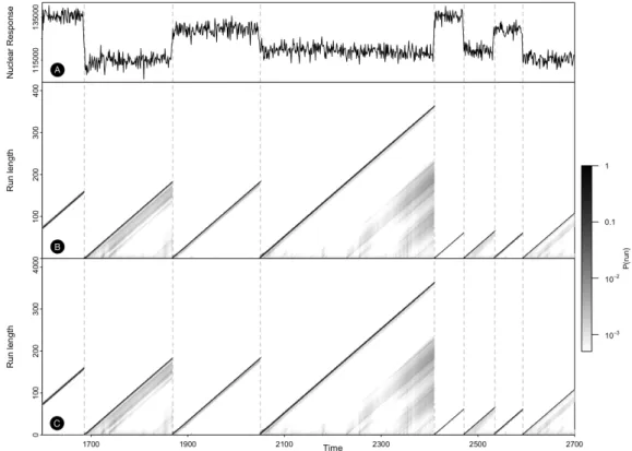
Figure 1. Changepoint detection results for the Well Log data. (A) A subset of data analysed with Online Bayesian Changepoint Detection algorithm. (B) The results obtained with our proposed method based on Sequential Importance Sampling. (C) The results obtained with [1] and [6] algorithms using conjugate priors. Both (B) and (C) depict the posterior run length over data observed so far,P(rt|x1:t). Darker points suggest run lengths with higher probability.
To minimise the effect of population degeneration issues, we use a Gaussian mixture approx-imation to the previous posterior as the proposal distribution. This mixture model prevents direct reusing of old samples from one generation to the next one. The variance scaling param-eter α in Algorithm 3.2 controls the scale of the kernel for a smoothing approximation of the proposal distribution with a Gaussian mixture model. It is usually chosen in the range of 0.1 – 1 and can be tuned individually to every application to obtain more effective proposal. We also measure the Effective Sample Size [12] of the obtained sample, and force resampling with replacement of the population when this metric drops below an arbitrarily selected threshold of M/2. This resampling allows us to drop low weight particles in the tails of the posterior, and focus more on high posterior density regions.
In practice we observed that the largest divergence between the proposal and the target distributions is frequently observed when sampling for the very first datum in the sequence using a prior sample as the proposal. In our case studies the resulting Effective Sample Size in such cases drops to about 20% of the Effective Sample Sizes observed later along the sequence of posteriors. We found it was better to use larger sample sizeM when the target posterior is conditioned on only one datum. In more complex cases a partial rejection control strategy [13] may be implemented to address the issues of large mismatch between the proposal and the target
distributions.
4
Experimental Results
We apply the proposed algorithm to three data sets. In the first two examples, we replicate results of [1] and analyse the data sets with our method for comparison. In the third example, our method is applied to a new data set to demonstrate how it performs with models without conjugate priors.
Well Log Data
A sequence of measurements of nuclear magnetic response was taken during the drilling of a well. The data are used to interpret geophysical structure of the rock surrounding the well. The variations in mean reflect the stratification of the earth’s crust. These data were earlier considered by [15] and [5].
A normal model with fixed variance σ2 = 40002 is used as an underlying generative model for the data. The model is parametrised by single parameterµthat corresponds to the mean of the normal distribution. To compare our results to those of [1] we use the same normal prior for µ, with hyperparameters µ0 = 1.15×10⁵, and σ02 = 1×10⁸. A memoryless changepoint prior
was chosen using the geometric distribution and corresponding hazard function H(rt) = 1/λ,
whereλ= 250.
A subset of the data is depicted in Figure 1. Panel A shows the original data values. Panel B shows the results obtained using the Sequential Importance Sampling approach proposed in this paper. Panel C shows the results obtained with the original Online Bayesian Changepoint Detection algorithm using conjugate priors. Notice that the drops to zero run length correspond well with the abrupt changes of the mean of the data. The differences between the results in Panel B and Panel C are very small and correspond to Monte-Carlo approximations in Sequential Importance Sampling and evaluation of the predictive distributions in (6), the mean square error between these results is 1.14×10⁻⁶. Samples of 1024 particles were used in this example for larger data sets, while samples of 4096 particles were used for samples from the prior and samples for the run lengths of 1. The smallest Effective Sample Size [12] is 351, which demonstrates that there were no population degeneracy problems in the sampler. Slightly lower effective sample sizes are observed immediately after a sudden change in the mean of the data, as these cases correspond to significant updates of the parameter posteriors.
Coal Mining Disasters
To demonstrate how our method works with count data and large data sets, we applied it to a data set containing the dates of coal mining explosions that killed ten or more men between March 15, 1851 and March 22, 1962 [11]. Following [1], the data were modelled with a Poisson process by weeks, with Gamma(1,1) prior on the rate. A geometric prior on the frequency of changepoints was selected with corresponding hazard functionH(rt) = 1/1000.
The results are plotted in Figure 2. The top panel shows the cumulative number of accidents. The middle panel shows the results obtained with the proposed algorithm using Sequential Importance Sampling. The bottom panel shows the results with the original Online Bayesian Changepoint Detection algorithm using conjugate priors. The results are again very similar,
Figure 2. Changepoint detection results for the Coal Mining Disasters data. (A) The cumulative number of significant coal mining accidents between 1851 and 1962. (B) The results obtained with our proposed method based on Sequential Importance Sampling. (C) The results obtained with [1] and [6] algorithms using conjugate priors. Both (B) and (C) depict the posterior run length over data observed so far, P(rt|x1:t). Darker points suggest run lengths with higher
probability.
with only minor differences caused by Monte-Carlo estimation of predictive probabilities, the mean square error between the two results is 3.02×10⁻⁸. A significant changepoint in the rate of coal mining disasters is usually attributed to the Coal Mines Regulations Act 1887 [16] that commenced as law on January 1st, 1888. This date corresponds to week 1930 in our data set and is marked in the plots with a dashed line.
As the data set contains 6000 time points, 6000 run length updates need to be performed in an online setting, and importance sampling procedure had to be performed N(N −1)/2 = 17,997,000 times. To keep the algorithm execution time reasonable, we were using small sample sizes of only 256 particles. The smallest effective sample size in these populations was 47, this demonstrates that we avoided population degeneracy problems [12].
Gold Prices
To demonstrate how our proposed method works with models without conjugate priors, we applied it to a new data set containing the closing prices of gold measured in USD/oz from 16th July 2014 to 16th July 2015. The data are available in the supplementary material to this
paper. The data were modelled with a stochastic differential equation, dG=µGdt+σGdW,
where G is the price of gold, µ and σ2 are the drift and stochastic volatility parameters
re-spectively, and W is a Wiener process. This equation is often used in financial modelling to describe asset prices under the assumption that prices only depend on the present and not on the past states of the market. This model belongs to a class of stochastic processes known as Itˆo processes [10]. A significant result for such processes, known as the Itˆo lemma [9], allows us to derive an expression for the functions of G(t). Using this lemma, logarithms of G(t) are given as dlogG= ( µ−σ 2 2 ) dt+σdW.
Integrating this equation over the interval [t, t+ 1] gives logG(t+ 1)−logG(t) = ( µ−σ 2 2 ) +σZt,
whereZt∼ N(0,1). Using the properties of the normal distribution we can write
logG(t+ 1)−logG(t)∼ N(µ−σ 2 2 , σ 2), logG(t+ 1) G(t) |µ, σ 2 ∼ N(µ−σ2 2 , σ 2).
Hence, we can model daily returns using a lognormal distribution with location µ−σ2/2 and scaleσ.
The parameters µ and σ2 were considered unknown random variables, and were assigned weakly informative prior distributions based on previous knowledge of gold prices. Using data for gold prices from 1968 to 2013, it was concluded that the rate of daily returns changes slightly from day to day at a maximum of ±0.7%. The mean rate of returns is expected to have higher density closer to zero, and lower density for larger deviations. As a result, we assigned a normal prior to µ with mean µ0 = 0 and variance σ02 = 0.0052 = 2.5×10⁻⁵. Based on the observed
volatility of the historic prices, we selected an exponential prior for the volatility parameter σ2 with mean 2.5×10⁻⁵. A memoryless changepoint prior was chosen using the geometric distribution and corresponding hazard functionH(t) = 1/λ, where λ= 100.
Figure 3 shows the result of changepoint analysis performed using the proposed algorithm. The most likely outcome is that the observations begin in a state with negative drift and a relatively low volatility of the prices, then some time between 8 October 2014 and 5 November 2014 the market switches to approximately zero drift with high volatility, finally, in the second half of May 2015 the market goes back to a negative drift and low volatility regime.
Significant changes in the distribution of parameter posteriors with more data becoming available required using larger populations in Sequential Importance Sampling to tackle popula-tion degeneracy problems. After a few trials with smaller populapopula-tions and observing low effective sample sizes, we ended up using a population of 32768 particles for the posteriors corresponding to run length from 0 to 30, and populations of 2048 particles for posteriors corresponding to longer run lengths. The minimal effective sample size achieved with this configuration is 426, which shows no evidence of population degeneracy problems.
Figure 3. Changepoint analysis of the gold prices during 2014–2015. The closing market price of gold in USD/oz is plotted in the top panel. The lower panel depicts posterior run length probabilities at different dates.
5
Discussion
The main structure of the proposed algorithm is similar to the one published by [1] and [6]. Sampling from the posterior of model parameters with Sequential Importance Sampling, instead of using conjugate prior updates, enables our method to perform changepoint detection with models that do not have conjugate priors. Avoiding conjugate priors also allows informative priors based on existing knowledge or observations of similar data to be used for changepoint detection in a truly Bayesian way.
[6] suggested the idea of numerical integration, and earlier gave an example of such ap-proach using MCMC in [4]. The proposed Sequential Importance Sampling apap-proach provides a different sampling scheme to aid such numerical integration which does not suffer from common MCMC convergence problems and can be easily implemented in high performance computing environment.
The computational complexity of processing one more data point grows linearly as new data arrive, as with every datum one more run length needs to be considered. The requirements for data storage in computer memory also grow linearly. The computational complexity of the proposed algorithm is on the same order as for the algorithms of [1] and [6]. It must be noted that performing importance sampling is more computationally expensive in comparison to updating conjugate parametrisation. Updating conjugate parametrisation typically takes just a small constant number of arithmetic operations. Resampling the parameter posterior with SMC for a sample size M takes O(M2) operations and therefore produces large complexity scaling constants. Therefore the proposed algorithm is slower than the one that uses conjugate priors with a constant complexity proportion. For example, performing the last round of updates in the Well Log example takes the original Online Bayesian Changepoint Detection algorithm
0.000155 seconds, while our algorithm requires 5.64293 seconds. This shows that our algorithm is almost 40,000 times slower. However, Sequential Monte Carlo methods are well suited for parallel implementation using high performance computational resources, as all of the particles in the population are sampled independently and therefore can be processed at the same time. The source code provided in the supplementary material implements Sequential Importance Sampling for the three examples described in this paper using three approaches: a traditional sequential implementation, a multiprocessor parallel algorithm using OpenMP framework, and a massively parallel implementation running on a graphics processor via CUDA framework.
The examples considered in this paper use models with a small number of parameters. Un-fortunately, it is well known that importance sampling is usually inefficient in high-dimensional spaces [7]. So, as the number of model parameters increases, the problem with arise in this setting. However, the number of parameters needed to observe these problems is quite high, and in many practical applications medium sized models will still be feasible.
In real world applications some heuristic simplifications can be made to limit the computa-tional complexity of the problem. Only limited run lengths may need to be considered when monitoring some data. For example, processing the Well Log data set, we could have limited the maximal run length time to the order of a few hundred as we expect changepoints to occur on average every 250 time points. Another example would be monitoring fast changing financial markets, where the possibility of a run that goes over several years is practically zero.
Acknowledgement
We are grateful to Prof Dirk Husmeier and Benn MacDonald for their valuable suggestions and comments made while preparing this paper for publication.
Bibliography
[1] Adams, R. P. and MacKay, D. J. C. (2007)Bayesian online changepoint detection. arXiv preprint, arXiv:0710.3742.
[2] Barry, D. and Hartigan, J. A. (1992) Product partition models for change point problems. The Annals of Statistic,20, 260–279.
[3] Barry, D. and Hartigan, J. A. (1993)A Bayesian Analysis of change point problems.Journal of the American Statistical Association,88, 309–319.
[4] Fearnhead, P. (2006)Exact and efficient Bayesian inference for multiple changepoint prob-lems.Statistics and Computing, 16(2), 203–213.
[5] Fearnhead, P. and Clifford, P. (2003)On-line inference for hidden Markov models via par-ticle filters. Journal of the Royal Statistical Society: Series B (Statistical Methodology),
65(4), 887–899.
[6] Fearnhead, P. and Liu, Z. (2007)On-line inference for multiple changepoint problems. Jour-nal of the Royal Statistical Society: Series B (Statistical Methodology),69(4), 589–605. [7] Doucet, A., de Freitas, N. and Gordon, N. (2001) Sequential Monte Carlo Methods in
[8] Green, P. J. (1995)Reversible jump Markov chain Monte Carlo computation and Bayesian model determination.Biometrika,82(4), 711–732, Biometrika Trust.
[9] Itˆo, K. (1944) Stochastic Integral.Proceedings of the Imperial Academy, 20(8), 519–524. [10] Itˆo, K. and McKeen Jr., H. P. (1974)Diffusion Processes and Their Sample Paths.Springer,
Berlin.
[11] Jarrett, R. G. (1979)A note on intervals between coal-mining disasters.Biometrika,66(1), 191–193.
[12] Kong, A., Liu, J. S. and Wong, W. H. (1994)Sequential imputations and Bayesian missing data problems.Journal of the American Statistical Association,89, 278–288.
[13] Liu, J. S. (2001) Monte Carlo Strategies in Scientific Computing.Springer, Berlin.
[14] Liu, J. S., Chen, R. and Wong, W. H. (1998) Rejection control and sequential importance sampling.Journal of the American Statistical Association, 93(443), 1022–1031.
[15] ´O Ruanaidh, J. J. K. and Fitzgerald, W. J. (1996)Numerical Bayesian methods applied to signal processing.Springer, New York, 0-387-94629-2.
[16] Peace, M. W. (1888)Coal Mines Regulation Act, 1887. 50 & 51 Victoria, Cap. 58., Lorimer and Gillies, London.
[17] Saat¸ci, Y., Turner, R. D. and Rasmussen, C. E. (2010) Gaussian process change point models.Proceedings of the 27th International Conference on Machine Learning (ICML-10), 927–934.
[18] Smith, A. F. M. (1975)A Bayesian approach to inference about a change-point in a sequence of random variables.Biometrika,62(2), 407–416.
[19] Stephens, D. A. (1994) Bayesian retrospective multiple-changepoint identification.Applied Statistics,43, 159–178.
[20] Turner, R. D., Bottone, S. and Stanek, C. J. (2013) Online Variational Approximations to non-Exponential Family Change Point Models: With Application to Radar Tracking. Advances in Neural Information Processing Systems, 306–314.