2012
Pseudo-random number generators and an
improved steganographic algorithm
Donald Peterson
Iowa State UniversityFollow this and additional works at:
https://lib.dr.iastate.edu/etd
Part of the
Mathematics Commons
This Thesis is brought to you for free and open access by the Iowa State University Capstones, Theses and Dissertations at Iowa State University Digital Repository. It has been accepted for inclusion in Graduate Theses and Dissertations by an authorized administrator of Iowa State University Digital Repository. For more information, please [email protected].
Recommended Citation
Peterson, Donald, "Pseudo-random number generators and an improved steganographic algorithm" (2012).Graduate Theses and Dissertations. 12797.
by
Donald Christopher Peterson
A thesis submitted to the graduate faculty
in partial fulfillment of the requirements for the degree of MASTER OF SCIENCE
Major: Applied Mathematics
Program of Study Committee: Jennifer L. Davidson, Major Professor
Clifford Bergman Eric Weber
Iowa State University Ames, Iowa
2012
DEDICATION
To Mary
TABLE OF CONTENTS
LIST OF TABLES . . . v
LIST OF FIGURES . . . vii
ACKNOWLEDGEMENTS . . . ix ABSTRACT . . . x CHAPTER 1. INTRODUCTION . . . 1 1.1 Background . . . 1 1.2 Definitions . . . 3 1.3 JPEG compression . . . 4 1.3.1 RGB toY CrCb . . . 6
1.3.2 Division of pixels into blocks . . . 7
1.3.3 Discrete cosine transform . . . 8
1.3.4 Quantization . . . 9
1.3.5 Encoding and compression . . . 10
1.3.6 Decompression into spatial domain . . . 11
1.4 Steganography . . . 11 1.4.1 Steganographic security . . . 12 1.4.2 Measuring distortion . . . 13 1.4.3 LSB replacement . . . 14 1.4.4 Permutative straddling . . . 15 1.5 Steganalysis . . . 17 1.5.1 Pattern classifiers . . . 18
1.6.1 1/P pseudo-random number generator . . . 24
1.6.2 Predictability of 1/P . . . 26
1.7 The psteg algorithm . . . 26
CHAPTER 2. STEGANOGRAPHIC ALGORITHMS . . . 31
2.1 F5 and nsF5 . . . 32
2.2 MB1 and MB2 . . . 35
2.3 Steghide . . . 36
CHAPTER 3. PSTEG ALGORITHM DESIGN . . . 38
3.1 Proposed design for psteg . . . 38
3.2 Image Database . . . 44
3.3 Steganalyzer . . . 44
3.3.1 POMM features for steganalysis . . . 45
CHAPTER 4. EXPERIMENTS AND RESULTS . . . 49
4.1 Experiment design . . . 49
4.1.1 Data generation . . . 49
4.1.2 Pattern classifier design . . . 50
4.1.3 Multi-classifier design . . . 51 4.2 Results . . . 53 4.2.1 Training data . . . 53 4.2.2 Testing data . . . 61 CHAPTER 5. CONCLUSION . . . 68 BIBLIOGRAPHY . . . 70
LIST OF TABLES
Table 1.1 The spatial domain data of an image (top) and its frequency domain data after JPEG compression at 75% quality (bottom). . . 5
Table 1.2 An example binary payload m embedded into a spatial-domain cover imagexby LSB replacement to produce the stego image y. . . 16 Table 1.3 The number of changesnc required to embedmintoxˆ1 andxˆ2. . . 27 Table 2.1 The truth table for the "exclusive or" (⊕) operation. . . 34
Table 3.1 The computed embedding efficiency of the psteg1 and psteg2 algorithms. 44
Table 4.1 The fifteen binary pattern classifiers. . . 50
Table 4.2 Example output of the 15 SVMs and the multi-classifier’s classification for example1.jpg. (c = cover, m = MB2, n = nsF5, 1 = psteg1, 2 = psteg2,s= Steghide) . . . 52
Table 4.3 Example output of the 15 SVMs and the multi-classifier’s classification for example2.jpg. (c = cover, m = MB2, n = nsF5, 1 = psteg1, 2 = psteg2,s= Steghide) . . . 52
Table 4.4 Correct classification rates for the binary SVMs against training data. Each column shows the rates against a particular SVM. For example, the highlighted cells show the correct classification rates for nsF5 and psteg1 images analyzed by the nsF5 vs. psteg1 SVM. . . 55
Table 4.5 Probability of classification errorPE = 12(PF A+PM D)for each algorithm
measured on training data. . . 57
Table 4.7 Correct classification rates for the binary SVMs against testing data. . 62
Table 4.8 Probability of classification errorPE = 12(PF A+PM D)for each cover vs.
algorithm SVM measured on testing data. . . 64
LIST OF FIGURES
Figure 1.1 The basis patterns of the DCT. . . 8
Figure 1.2 A lossless format image (left) compressed to a JPEG image at 90% qual-ity (center) and 10% qualqual-ity (right). . . 10
Figure 1.3 The zig-zag vector order for an 8-by-8 block of DCT coefficients during encoding. . . 11
Figure 1.4 An 8-bit grayscale imagex and its spatial bitplanesxi. . . . 15
Figure 1.5 A simulation of embedding in lexicographical order without permutative straddling. . . 17
Figure 1.6 A simulation of embedding in lexicographical order with permutative straddling. . . 17
Figure 1.7 A set of verticesV = (V1, . . . , V7), a cyclic digraph(E1, V)pictured left, and an acyclic digraph (E2, V) pictured right. . . 21 Figure 1.8 The logarithm of the number of golden permutations as a function of
cover size nand payload sizel. . . 29
Figure 2.1 The steganographic value of DC coefficients as defined by F4. . . 33
Figure 3.1 A flow chart illustrating the partitioning of an image. . . 39
Figure 3.2 A simulation finding the optimal match of payload to coefficients in a partition. . . 41
Figure 3.3 A chart describing how quantized AC coefficients can change in the psteg1 algorithm. . . 42
Figure 3.4 A chart describing how quantized AC coefficients can change in the psteg2 algorithm. . . 42
Figure 3.5 The first 5 of 47 partitions during psteg embedding usingP = 503, four bases, partition threshold t = 0.1, and an embedding rate of 0.1 bpnz. The image is a 512-by-512, 8-bit, grayscale JPEG compressed at quality factor 75 from the BOSS database. It contains 24290 nonzero, quantized AC coefficients. . . 43
Figure 4.1 The creation of the training and testing data from the BOWS2 database. 50
Figure 4.2 The process of training a binary SVM. . . 51
Figure 4.3 Correct classification rates for the binary SVMs against training data. . 56
Figure 4.4 Probability of classification errorPE = 12(PF A+PM D)for each algorithm
measured on training data. . . 57
Figure 4.5 Correct classification rates for the multi-classifier against training data. 60
Figure 4.6 Correct classification rates for the binary SVMs against testing data. . 63
Figure 4.7 Probability of classification errorPE = 12(PF A+PM D)for each algorithm
measured on testing data. . . 64
ACKNOWLEDGEMENTS
I would like to take this opportunity to express my gratitude to everyone who helped me throughout the research and writing of this thesis. First, I give my utmost thanks to Dr. Jennifer Davidson for giving me direction, inspiration, her time, and her patience over the past two years. I would like to thank Dr. Clifford Bergman for driving my interest in mathematical research throughout the entirety of my academic career, and Dr. Eric Weber for pushing me to think like a mathematician.
It gives me great pleasure to thank Dr. John VanDyk for his wisdom, mentorship, and the provision for me to continue my education. I would like to thank my friends for their patience and tolerance regarding my rants on the beauty of prime numbers, and Lorry VerSteeg for providing me with the energy needed to complete this thesis and a haven in which to work. Last, but not least, I deeply want to thank my family for their unremitting, unyielding, oft undeserved, and unparalleled support and confidence.
ABSTRACT
Steganography is the art and science of hiding secret information in a cover medium such that the presence of the hidden information cannot be detected. This thesis proposes a new method of steganography by cover modification in JPEG images. Essentially, the algorithm exercises LSB replacement using the definition for steganographic values from F5. After the nonzero quantized DCT coefficients of a cover image undergo a pseudorandom walk, the coefficients and the payload are split into an equal number of partitions and paired. Each coefficient partition is permuted again by the 1/P pseudo-random number generator until an optimal embedding efficiency for its corresponding payload is achieved. Using this method, we achieve a higher embedding efficiency than that of LSB replacement alone. We evaluate the detectability of our algorithm by creating a multi-classifier based on the output of multiple non-linear, soft-margin support vector machines trained on POMM features. We show that our algorithm performs nearly as well as the state-of-the-art nsF5 algorithm, and outperforms other state-of-the-art algorithms under most conditions.
CHAPTER 1. INTRODUCTION
1.1 Background
Suppose that Alice and Bob are two prisoners in separate cells of a prison. They are allowed to communicate with each other indirectly through messages, but all communications are monitored by the warden, Eve. Alice wants to plan an escape with Bob, but they must communicate discretely because Eve will throw them both into solitary confinement if she discovers that hidden messages are being shared between them. Knowing that these were likely to be the conditions in prison, Alice and Bob agreed on a secret key before they were thrown into prison. They use this key to hide their covert messages in seemingly innocuous communication with the hopes of not arousing Eve’s suspicion.
We assume that Eve, having been warden for many years, knows the tricks that prisoners often use to conceal their communication. Eve does not necessarily need to know the details of the escape to foil their plans; she only needs to know that secret messages are being sent between the two prisoners.
The prisoner’s problem [19] is often used to demonstrate the concept of steganography, or the art of concealing the presence of a message. This should not be confused withcryptography, which is the art of concealing the content of a message. Steganography aims to disguise the existence of a message altogether. While a steganographic system, or stegosystem, can be as simple as writing a message in invisible ink, modern steganography typically involves the use of digital multimedia as the message medium. Specifically, the steganographic algorithms discussed in this thesis are concerned with hiding binary strings, orpayloads, in JPEG format digital images.
down into three categories: cover selection, cover synthesis, and cover modification [9]. The first two categories, while valid, are not considered practical by most means. Alice could choose her cover image so that it matches her payload, but this requires that she has access to a cover object for every possible payload she wishes to communicate. In a cover synthesis scenario, Alice creates a cover image that perfectly matches her payload. Unfortunately, dependencies between pixels in naturally occurring images make this method difficult to perform in practical-use scenarios. Most modern algorithms choose the third option, cover modification, to embed a payload by changing a cover object in such a way that a message can be extracted by someone who knows where to look. Algorithms are designed to minimize distortion while maintaining a respectable embedding capacity. The most common location for embedding information is in the least significant bit plane of an image.
The motivation behind this thesis is simple. We assume that the payload we want to embed is encrypted, so that it is composed of approximately equal proportions of the number 0 and the number 1. The least significant bits of nonzero AC coefficients of many, but certainly not all, JPEG images occur with an approximately equal (within 10%) distribution. The root of the problem, then, lies in the fact that the least significant bits just happen to be in the wrong order for our payload (with probability 1−1/2n, where n is our payload length). Thus, we
strategically modify the cover image to hide our payload. Depending on the efficiency of the embedding algorithm used, we change k bits of the cover image to hide n bits of payload. However, if we were able to find a permutation of the cover image’s elements that matched our payload exactly, and were furthermore able to communicate how to find the “embedded" payload, no changes to the cover image would be required. This steganography would be considered perfectly secure. Computationally, this is a very complex problem. In this thesis, we attempt to leverage predictable, yet still statistically sound, pseudo-random number generators to construct such a permutation.
In chapter 1, we give definitions and lay framework for many of the terms and concepts seen throughout the paper. In chapter 2, we review the mechanics behind some state-of-the-art embedding algorithms. We define our proposed algorithm, psteg, and our steganalyzer in chapter 3. In chapter 4, we compare the security and overall effectiveness of psteg against that
of the algorithms explored in chapter 2. We conclude with chapter 5.
1.2 Definitions
We refer to thenatural numbers Nas the set of integers greater than zero,N={0,1,2, . . .}. Fixb∈Z+ as a positive integer. Let the set of base b, or b-ary, numbers be defined as the set
sb = {q ∈ N | q < b} = {0, . . . , b−1} of natural numbers less than b. Let r ∈ R be a real
number. The base b representation of r is defined uniquely as the sequence of b-ary numbers
sr,b. We refer to an element ofsr,b as adigit, and we refer to the length of sr,b as the number
of digits in the sequence sr,b. Thus, the kth digit ofsr,b has the formsr,b(k). The decimal, or
base 10, representation of anyb-ary sequencesr,b of length nis defined as the sum n
X
k=1
sr,b(k)·bd−k (1.1)
whered is the number of elements insr,b describing the integer part ofr. Note that ifr is an
integer, thend=n. For example, letr= 231.75. The unique sequence expressingr in base ten issr,10= (2,3,1,7,5). To verify, letb= 10,n= 3, and sr,10= (2,3,1,7,5). By1.1, we have
n X k=1 sr,b(k)·bd−k= 5 X k=1 sr,10(k)·103−k =2·102+3·101+1·100+7·10−1+5·10−2 = 231.75
In the binary, or base 2, system, sr,10 = (2,3,1,7,5) is uniquely expressed by the sequence
sr,2 = (1,1,1,0,0,1,1,1,1,1). This can be verified by calculating the decimal representation of
sr,2. n X k=1 sr,b(k)·bd−k= 10 X k=1 sr,2(k)·28−k =1·27+1·26+1·25+0·24+0·23+1·22 +1·21+1·20+1·2−1+1·2−2 = 231.75
For an integer q, every element of sq,2 is referred to as a bit. An n-bit integer is an integer that can be expressed in n or fewer bits. Equivalently, the set of n-bit integers is defined as
{q ∈N|q <2n}={0,1, . . . ,2n−1}. We can see that231 = (11100111)
2is an 8-bit integer, but 256 is not, since256 = 28= (100000000)
2 requires nine bits to describe it. In big-endian binary notation, bits are ordered left-to-right by significance, with the most significant bit written first (left-most) and the least significant bit written last (right-most). This thesis will exclusively use big-endian notation. The most significant bit ofqis the most weighted element of the sequence
sq,2 and is denoted by q(1). The least significant bit, or LSB, of q is the last element of sq,2,
q(n), and is equivalent to its parity bit. The LSB of q can be explicitly defined by
LSB(q) =q mod2 = 0 if q is even 1 if q is odd. (1.2)
We define an image as a functionf that maps an index domainX to a value setY. Iff is a grayscale image, then X={(i, j) | 1≤i≤M,1≤j ≤N} is the domain of locations along the image and Y is the set of possible light intensities. The Cartesian location (i, j) is defined as a pixel, and the intensityf(i, j) is called thepixel value.
1.3 JPEG compression
Raster image formats follow the convention defined above by sampling light intensities of an image inM×N locations and storing them in anM-by-N-by-Darray, whereDis dependent on the image format. Typically,D= 1for monochrome and grayscale images. Monochrome images require only 1 bit per pixel to store image data. Here, Y = {0,1}, where a pixel value of 0 represents black and 1 represents white. Grayscale images necessarily require more than 1 bit to describe their pixel values. In ann-bit image, pixel values range acrossF ={0,1,2, . . . ,2n−1},
where 0 represents black,2n−1 represents white, and intermediate values represent intensities
of gray.
In 1992, the Joint Photographic Experts Group introduced the JPEG image format [20]. The JPEG image format uses the discrete cosine transform (DCT) to transform image data from the spatial domain to the frequency domain. JPEG compression is a lossy compression,
Table 1.1 The spatial domain data of an image (top) and its frequency domain data after JPEG compression at 75% quality (bottom).
108 122 113 104 98 87 90 96 121 124 109 103 109 105 98 93 128 124 106 91 96 98 90 89 124 122 107 75 67 71 70 84 125 121 112 76 67 75 65 77 133 122 119 89 94 107 75 73 135 124 126 94 100 116 78 75 130 124 130 88 81 98 70 80 −28 21 7 1 −2 −1 1 0 1 −5 0 −1 1 0 −1 0 5 −2 −3 0 0 0 0 0 0 0 −1 0 0 0 0 0 −4 1 1 −1 0 0 0 0 0 0 0 0 0 0 0 0 0 0 0 0 0 0 0 0 0 0 0 0 0 0 0 0
meaning that some of the original data is lost during compression. When decompressed back to the spatial domain, the resultant image is an approximation of the original spatial domain data. The closeness of this approximation, or the quality of the JPEG compression, is inversely proportional to its file size. In this sense, a low quality JPEG yields a file small file size but creates a mediocre representation of the original image. However, even medium quality factor compressions produce accurate results while greatly reducing file size. This makes the JPEG an incredibly versatile image format and is a major reason that it is one of the most popular image formats currently available.
There are five steps that the JPEG compression algorithm goes through to transform a spatial domain image to the frequency domain. Note that an image must be decompressed and transformed back into the spatial domain before it can be viewed. Since the DCT is invertible,
the steps may be performed in reverse order to decompress the image, using the inverse DCT instead of the DCT. The compression/decompression algorithm is explained in the following five subsections.
1.3.1 RGB to Y CrCb
The human eye contains light receptors, called cones, that help the brain to distinguish colors. There are three types of cones, and each one is particularly sensitive to one of three colors: red, blue, and green. The RGB additive color model capitalizes on this human characteristic by representing color as a linear combination of red, blue and green light. Many light emitting devices use the additive color model to display colors, as well as do many image formats. For instance, the bitmap image format (file extension .bmp) stores color image data in anM×N×3
dimensional matrix, where each M ×N plane consists of intensity data for one of the three additive color channels.
Much of the data represented by the RGB color model is highly correlated and can be represented more efficiently for storage and transmission purposes in other color models. The JPEG image format uses the Y CrCb color model to achieve this. The luminance component,
Y, is defined as a linear combination of the three components from the RGB color model:
Y = 0.299R+ 0.587G+ 0.114B. (1.3)
The weight of each RGB component is scaled to match the sensitivity of the human eye to its respective color. The chrominance components are the differences between the RGB color component and the luminance:
U =R−Y (1.4)
V =B−Y. (1.5)
Y U V = 0.299 0.587 0.114 0.701 −0.587 −0.114 −0.299 −0.587 0.886 R G B . (1.6)
When the chrominance components U and V are scaled to be in the range of signed 8-bit integers, we refer to them as Cr and Cb, respectively. The transform from RGB to Y CrCb is
then defined as Y Cr Cb = 0 128 128 + 0.299 0.587 0.114 0.5 −0.419 −0.081 −0.169 −0.331 0.5 R G B . (1.7)
Since the human eye is more sensitive to differences of luminance intensity than differences of color intensity, the color channels may be subsampled to reduce file size, as will be explained in more detail in the next subsection. In addition to the JPEG format, analog television broadcasts transmit in Y CrCb due to the efficiency of the model. Old black-and-white televisions (which
are actually grayscale) display the luminance channel and discard the chrominance channels. Similarly, grayscale JPEG images only contain image data in the luminance channel.
1.3.2 Division of pixels into blocks
After the image is transformed from RGB to Y CrCb, the signals are ultimately divided into
blocks of 8-by-8 in preparation for the Discrete Cosine Transform. Since the human eye is far more sensitive to differences in luminance than in chrominance, the chrominance signals are often subsampled to achieve a higher compression. For this reason, color images are able to achieve higher compression ratios (original file size/compressed file size) than grayscale images. The image is first divided into blocks of 16-by-16 pixels. From this block, the luminance signal is always subdivided into four 8-by-8 blocks. The chrominance signal, however, may be subsampled into fewer than four 8-by-8 blocks. Subsampling is achieved by averaging two adjacent pixels. The direction of subsampling is either by row or by column.
If no subsampling occurs, then the chrominance signals are also subdivided into four 8-by-8 blocks. This is abbreviated to a 4:4:4 representation (4 blocks of luminance, 4 blocks of red
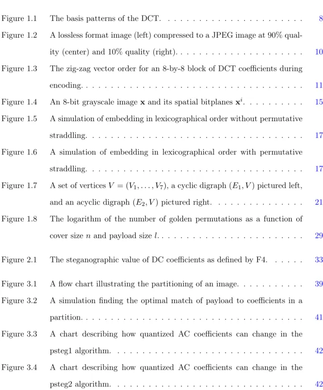
Figure 1.1 The basis patterns of the DCT.
chrominance, and 4 blocks of blue chrominance). If the 16-by-16 block is subsampled in both directions across both chrominance signals, the resultant division is a 4:1:1 representation. The chrominance signals may be subsampled across one or both directions and do not necessarily have to be subsampled in the same way directionally between the blue and red channels. In this sense, 4:2:2, 4:2:1, and 4:1:2 representations are also possible and can be defined for multiple directions.
1.3.3 Discrete cosine transform
The discrete cosine transform (DCT) changes spatial domain data into the frequency do-main. Each 8-by-8 block of pixels from the spatial domain can be expressed as a linear combi-nation of the basis patterns generated by the DCT, which are shown in Figure1.1. Each basis
pattern is referred to as a mode.
The coefficients d(k, l) of this linear combination, called DCT coefficients, are stored in 8-by-8 blocks, where k, l∈ {0, . . . ,7} They are calculated by the two-dimensional model
d(k, l) = 7 X i,j=0 w(k)w(l) 4 cos kπ 8 (i+ 1 2) cos lπ 8(j+ 1 2) B(i, j) (1.8)
where B(i, j), i, j ∈ {0, . . . ,7} are the 8-by-8 blocks of luminance or chrominance values,
w(0) = 1/√2, and w(k > 0) = 1. Note that d(0,0) is proportional to the average value
of the pixels in the spatial domain block, since
d(0,0) = 7 X i,j=0 w(0)w(0) 4 cos 0π 8 (i+ 1 2) cos 0π 8 (j+ 1 2) B(i, j) (1.9) = 7 X i,j=0 1 8 B(i, j) (1.10) = 7 X i=0 1 8 7 X j=0 1 8 B(i, j) (1.11) = 7 X i=0 1 64 7 X j=0 B(i, j) (1.12) = 1 64 7 X i,j=0 B(i, j). (1.13)
The coefficient d(0,0)is called the DC coefficient, and every other coefficient is referred to as a quantized AC coefficient. The DCT is invertible, and the two-dimensional inverse DCT is defined by B(i, j) = 7 X i,j=0 w(k)w(l) 4 cos kπ 8 (i+ 1 2) cos lπ 8 (j+ 1 2) d(k, l). (1.14) 1.3.4 Quantization
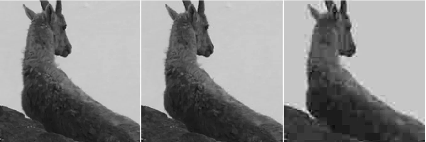
Once the data has been transformed into the frequency domain, every 8-by-8 block undergoes point-wise division by an 8-by-8 quantization matrix, and the resultant matrix is rounded to the nearest integer. This is the lossy step of the JPEG compression algorithm where some of the original spatial data may be lost. The JPEG format provides specification for 100 "standard" quantization matrices of different quality factors. After compression and decompression, the 90% quality quantization matrix Q90 yields a very close approximation to the original image data, while the 10% quality quantization matrix Q10 shows visible distortion (Figure 1.2). However, the JPEG created with Q10 will have a significantly smaller file size than the one created withQ90.
Figure 1.2 A lossless format image (left) compressed to a JPEG image at 90% quality (center) and 10% quality (right).
All quantization matrices are computed from the 50% quality quantization matrix Q50:
Qqf = max{1,round 2·Q50· 1− qf 100 }, qf >50 min{255·1,roundQ50·50qf }, qf ≤50 (1.15)
where the boldface1 denotes an 8-by-8 matrix of all ones. Custom quantization matrices can be used in place of the standard matrices and are stored in the header of the image.
1.3.5 Encoding and compression
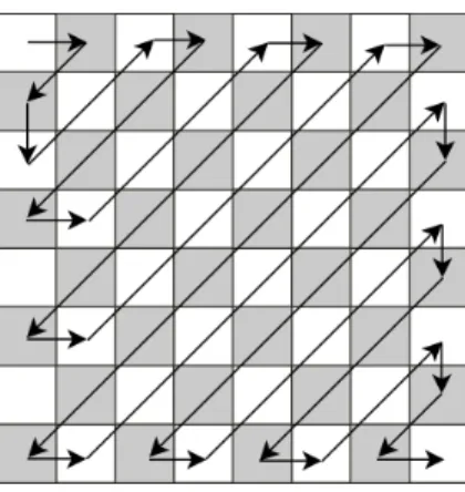
After quantization, the majority of the image data is concentrated toward the upper-left corner of the blocks. The high-frequency data (bottom-right corner of an 8-by-8 block) comprises the majority of the lost data from the lossy compression. Even at medium quality factor levels, over half of the coefficients in the 8-by-8 block will usually become 0. JPEG compression exploits this characteristic by reorganizing each block into a vector for Huffman encoding. Each vector starts with the upper-left most coefficient of the block which is called the quantized DC coefficient. Starting with this coefficient, the remaining coefficients, called quantized AC coefficients, are read in a zig-zag pattern towards the bottom-right hand corner of the block, as is shown in Figure1.3. Since the vectors are usually comprised of a long string of 0’s at the
Figure 1.3 The zig-zag vector order for an 8-by-8 block of DCT coefficients during encoding.
image data is typically encoded using the Huffman tables recommended by the JPEG standard, but custom tables may again be used and stored in the image header.
1.3.6 Decompression into spatial domain
To read a JPEG image, the data must first be transformed back into the spatial domain. This is done by performing the inverses of the above steps in reverse order. The encoded data is decoded using Huffman tables and restored into 8-by-8 blocks of the image. Each block is multiplied, not divided, point-wise by the same quality factor quantization matrix that was used during compression. Each block is run through the inverse DCT. If subsampling occurred, the subsampled channels are restored to full size. Lastly, the image data is transformed from theY CrCb color model back into the RGB color model.
1.4 Steganography
Let C be the set of all cover objects x ∈ C, M(x) be the set of all messages that can be embedded inx,K(x)be the set of all stego keys forx, andS(x) be the set of all possible stego images. A generalized stegosystem is a pair of functions (E,D)in which
E :C × M(x)× K(x)→ S(x); E(x,m, k) =y, (1.16)
where x ∈ C, y ∈ S(x), k,kˆ ∈ K(x), and m,mˆ ∈ M(x). Here, the embedding algorithm E
embeds a payload minto a cover object x in a manner that makes use of a stego key k. The output of E is y, which is called the stego object. The extraction algorithm D uses the stego keykˆ to extract the payloadmˆ fromy. Ifk= ˆk, thenm= ˆm.
The maximum size of the payload m is dependent on both the number of embeddable locations in the cover objectxand the embedding algorithm used. Ifxis anM-by-N grayscale image in the spatial domain, then every pixel location would be considered an embeddable location. If the embedding algorithm embeds one bit of information into every pixel, mhas a maximum length ofM N. However, ifxis anM-by-N JPEG grayscale image and payload bits are embedded into DCT coefficients, then the number of embeddable locations is most likely fewer thanM N since most algorithms avoid embedding into quantized AC coefficients of value 0. The number of quantized AC coefficients of value 0 depends on both the content of the image and the quality factor quantization matrix used during compression. Thus, the number of possible embedding locations of an imagex in the frequency domain is highly variable. The
embedding rate expresses the relative payload size and is defined as the ratiol/n, wherelis the number of bits in the payload and nis the number of embeddable elements in the image.
We assume, in general, that the payload is compressed and encrypted in order to minimize the distortion caused by the embedding process. Compression minimizes the size of the mes-sage, while encryption of the payload secures the message and also gives the payload desirable statistical properties. If the cryptosystem is secure, resultant payload bits will be uniformly distributed and the payload will share properties with a truly randomized bitstring.
1.4.1 Steganographic security
A stegosystem is considered secure if there is no way for an attacking third party (Eve) to distinguish cover objects from stego objects. To put this into more quantitative terms, we must first formalize what it means for Eve to "distinguish a cover object from a stego object." Suppose that prisoners are only allowed to communicate with 8-bit, m-by-ngrayscale images. If Eve observes what she knows to be legitimate, innocent communication over a long enough time, she will eventually be able to model a probability distribution Pc over the space of all
cover images C ={0, . . . ,255}m×n. Similarly, if Alice and Bob are communicating in secret, a
different distributionPsoverCcan be modeled with a sufficiently large sample of their messages.
Borrowing Kerckhoff’s principle from cryptography, we assume that Eve knows Pc,Ps, and
the steganographic channel used. In other words, she knows what cover (innocent) images look like, she knows what stego images look like, and she even knows the particular stegosystem that Alice and Bob are using. Using some metric, Eve measures how closely related the two distributions Pc and Ps are. If Pc and Ps are very distinct, then she should be able to easily
classify a given image as being either a cover image or a stego image. However, if Pcis “close"
to Ps, then she is more prone to making errors in classification of the image.
Often in information theory, two distributions P1 and P2 are compared by measuring the Kullback-Leibler divergence DKL(P1||P2) = X x∈C P1(x) log P1(x) P2(x) . (1.18)
If Alice uses a stegosystem that creates stego objects with distribution Ps that is identical
to the Eve’s distribution of cover objects Pc, then by (1.18) we haveDKL(Pc||Ps) = 0. Such a
stegosystem is calledperfectly secure as Eve has no way to distinguish cover objects from stego objects. While some perfectly secure stego systems exist, they typically require assumptions that contradict practical usage scenarios [9]. A stegosystem that satisfies DKL(Pc||Ps) ≤ is
called an -secure stegosystem.
1.4.2 Measuring distortion
Generally speaking, steganographic embedding algorithms need to modify a cover object in order to hide a payload in it. We call these modifications distortions. The less an image is distorted, the less likely it is to be detected by a steganalyst. Typically, the distortion between a cover object x and stego imagey=E(x,m,k) is measured by a distortion function d(x,y), whered:C ×C →[0,∞). One such distortion function measures the total number of embedding changes and can be defined as
ν(x,y) =
n
X
i=1
whereδ is the Kronecker delta δ(x(i)−y(i)) = 1 when x(i)−y(i) = 0 0 when x(i)−y(i)6= 0 (1.20)
and nis the number of embeddable locations in x. For simplicity, we use a single index ithat ranges across all pixel locations.
Another useful statistic for quantifying the effectiveness of a stegosystem is the expected embedding efficiency,e, of the embedding algorithm. This is defined as the expected number of payload bits embedded per average embedding distortion
e= Ex[log2|M(x)|]
Ex,m[d(x,y)]
, (1.21)
where|M(x)|is the number of bits in the payload. The efficiency of an algorithm is sometimes dependent on the specific processes that algorithm uses and the set of cover objects it acts upon. As such, it sometimes becomes rather difficult to compute the expected efficiency of an algorithm. If this is the case, it is determined experimentally.
1.4.3 LSB replacement
LSB embedding is one of the simplest methods for embedding information into cover object, and it is the most popular mechanism in use among state-of-the-art steganographic systems. It utilizes the least significant bit of an embedding location as its means of communication. A naive embedding algorithm that uses this method is called LSB replacement, in which the LSBs of a cover object’s embedding locations are overwritten with the desired binary payload.
Let x ∈ C be a cover image with c embeddable locations. Let the image data be of the format n-bit integers, such that each pixel value xi can be expressed in n bits as sxi,2 = (sxi,2(1), . . . , sxi,2(n)) andxi =
Pn
k=1sxi,2(k)·2
n−k. Suppose that we wish to embed a binary
message m∈ {0,1}l of lengthl intox using LSB replacement, where l < c. The LSB
replace-ment embedding algorithm creates a stego imagey∈ C that is identical tox, except it changes the LSBs of the first l embeddable locations in y to match that of the message m. In other words, the most significant b−1 bits of every element of y are the same as x, but the LSB of
Figure 1.4 An 8-bit grayscale imagexand its spatial bitplanes xi.
the first l embeddable locations may differ, since the LSB of theith embeddable location of y
is given by LSB(yi) = mi if0< i≤l LSB(xi) ifi > l (1.22)
Analogously, the LSB replacement algorithm overwrites the LSBs of the firstl pixels inxwith the payload m. Since the LSB bitplane is noisy to begin with (Figure 1.4), one hopes that the introduced distortion will blend in with the rest of the plane. This, of course, requires the underlying assumption that the LSB plane of a cover image x is randomly and uniformly distributed. This is obviously not true for all images; a completely black image (every pixel
xi = 0) would be a poor choice of cover object for LSB replacement. However, never-compressed
natural images tend to adhere to this assumption due to random amounts of noise captured by the imaging device. Thus we assume that the LSBs of a given cover imagex are uniformly and randomly distributed throughout the plane. Furthermore, the assumption is made that the LSB of a pixel is independent of the other bits in the pixel.
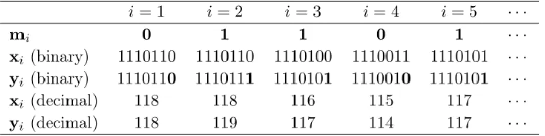
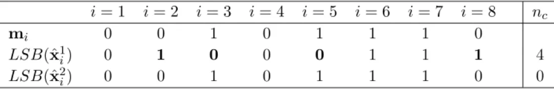
Table 1.4.3 demonstrates an example of the LSB replacement algorithm for the first five
pixels of a particular cover image x in the spatial domain and the first five bits of a payload
m. However, LSB replacement is not limited to images in the spatial domain. In the frequency domain, LSB replacement uses the LSBs of the non-zero quantized AC coefficients in the image.
1.4.4 Permutative straddling
Suppose that Alice uses an embedding algorithm to embed anl bit payload minto a cover image x with n embeddable elements, and suppose that l ≈ n/4. We assume that Alice will make changes to the image in order to embed the payload and, in doing so, will distort the
Table 1.2 An example binary payload m embedded into a spatial-domain cover image x by LSB replacement to produce the stego imagey.
i= 1 i= 2 i= 3 i= 4 i= 5 · · · mi 0 1 1 0 1 · · · xi (binary) 1110110 1110110 1110100 1110011 1110101 · · · yi (binary) 1110110 1110111 1110101 1110010 1110101 · · · xi (decimal) 118 118 116 115 117 · · · yi (decimal) 118 119 117 114 117 · · ·
stego image from the cover image. If she embeds the message into the first l pixel locations, or embeds in raster order, then the distortion is concentrated into a particular region of the image. However, if she spreads the payload bits evenly across the entirety of the cover image, the distortion is spread out and may be less noticeable.
Most embedding algorithms use a pseudo-random number generator to “randomly" select locations across the entirety of an image in which to embed information. In the prisoner’s problem, Alice and Bob both share knowledge of a secret key k. Suppose that Alice initializes a pseudo-random number generator with seed k to create a permutation σ. She permutes the embeddable locations in the cover imagexto createσ(x) = ˆx. Alice embedsmintoˆxto create the stego objectyˆ, and restores the permuted locations to their original order withσ−1(ˆy) =y. Once Bob receives y, he initializes the same pseudo-random number generator that Alice used withk to generateσ(y) = ˆy. He can then extract the message m.
Embedding algorithms tackle the problem of the payload distribution step in different ways. However, a pseudo-random permutation of the cover elements known aspermutative straddling
[21] is a computationally efficient method of uniformly distributing a payload across a cover. While the primary goal of permutative straddling lies in distributing the payload uniformly across a cover object, it subsequently avoids embedding sequentially into a potentially invariant region of the cover object. Consider embedding a payload into a spatial domain cover image without first permuting the elements of the cover. If the cover image is a picture taken outdoors, the possibility exists that the top of the image is a clear sky. Permutative straddling prevents heavily distorting this uniform region.
Figure 1.5 A simulation of embedding in lexicographical order without permutative straddling.
Figure 1.6 A simulation of embedding in lexicographical order with permutative straddling.
1.5 Steganalysis
Steganalysis, as opposed to steganography, is the science of detecting the presence of hidden content in images. Since most embedding algorithms alter images in a way that is nearly undetectable to the human eye, steganalysts use algorithms to scan an image for statistical anomalies that may have resulted from the embedding process. The term for such an algorithm is a steganalyzer.
Some embedding algorithms leave rather unique fingerprints on their stego objects, such as that of LSB replacement. Targeted steganalyzers are designed to analyze content for these trademark statistical anomalies. In general, a targeted steganalyzer is designed to look for a specific signatures that a specific embedding algorithm leaves behind. This requires knowledge of both the embedding algorithm used and the distinguishing statistics it leaves. For example, LSB replacement is highly detectable by the Chi-square attack [22]. As such, more sophisticated algorithms avoid the rather blatant anomalies caused by LSB replacement and therefore require
their own targeted steganalyzer based on another characteristic to be detected.
1.5.1 Pattern classifiers
Blind steganalyzers, on the other hand, attempt to detect the presence of hidden content with a single, blanketed attack. Typically, this involves reducing a high-dimensional image down to a lower-dimensional feature space and running statistical attacks on these features. The attacks are carried out by pattern classifiers, which are complex machine-learning algorithms. A binary pattern classifier used for image steganalysis will classify an input image as one of two possible categories based on its training data. While this is intuitively applicable to classify an image as either cover (innocent) or stego, it can also be applied to classify an image as being embedded with one of two stego algorithms. In this thesis, we construct a blind steganalyzer, which we refer to as a multi-classifier, using multiple binary pattern classifiers as the basis for classification. Given k steganographic embedding algorithms, we train k+12
binary classifiers on a feature set. Each classifier judges whether the input features of a given image belong to one of two categories drawn from our pool ofk+1total categories composed of thekembedding algorithms plus the possible verdict that the image is a cover (innocent).
1.5.1.1 Support vector machines
We use non-linear, soft-margin Support Vector Machines [4], or SVMs, as the binary clas-sifiers for our steganalyzer. A hyperplane is the generalization of a two-dimensional plane in three-dimensional Euclidean spaceR3 to that of a higher dimension, in that it partitions a set of elements mapped in higher-dimensional space into two disjoint sets. A hyperplane has the form
w·x−b= 0
wherexis a set of data vectors,wis the vector normal to the hyperplane,·is the dot product, and ||wb|| is the offset of the hyperplane from the origin alongw. SVMs map low-dimensional
feature set data to a higher-dimensional space and construct a hyperplane that partitions the data into two categories.
LetD=
(xi, yi) |xi ∈Rk, yi ∈ {−1,1} ni=1 be the set of all training data, wherexi is ak
-dimensional training vector andyi is its classification. In our case, the valuesxi will be POMM
features, defined in the next section and section 3.3.1. Ideally, the training data is linearly separable, and we want to maximize the distance between two hyperplanes that separate the training data. This optimization problem can be summarized as minimizing ||w||such that for
any i= 1, . . . , n, we have
yi(w·xi−b)≥1 (1.23)
However, our training data are usually not perfectly linearly separable. To account for this, slack variablesξi are used to measure the degree of classification error. Such an SVM is called
a soft margin SVM. The minimization problem then becomes
min w,ξ,b ( 1 2||w|| 2+C n X i=1 ξi ) (1.24)
such that for any i= 1, . . . , n,
yi(w·xi−b)≥1−ξi, ξi ≥0. (1.25)
Note that in (1.24), we use 12||w||2 in place of ||w|| to eliminate the square root for compu-tational purposes. C is a parameter describing the penalty for error. In the dual form of the optimization problem, the slack variables vanish. After introducing Lagrangian multipliers α, the optimization problem requires maximizing αi in
n X i=1 αi− 1 2 n X i,j=1 αiαjyiyjK(xi,xj) (1.26)
such that for any i= 1, . . . , n, we have 0≤αi ≤C and n
X
i=1
αiyi= 0.
Linear SVMs define the kernel as K(xi,xj) = xi ·xj, where · represents the dot
prod-uct. However, the image data that we are training is better separated by a non-linear kernel. Non-linear SVMs use one of many non-linear kernels to replace the dot product between two training vectors in the linear model. For our experiments, we chose the Gaussian Radial Basis Function defined asK(xi,xj) =exp(−γ||xi−xj||2), γ >0.The parameters for the penalty for
misclassification, C, and the kernel width, γ, are experimentally tested over a range of values to determine the optimal parameters for the SVM. We measure the accuracy of the SVM at every pair(C, γ) using a technique called cross validation.
With k-fold cross-validation, we first split the training set into k partitions. A model is generated from k−1 partitions, and the accuracy of the model is tested on the remaining partition. The same parameters are used to train on a different set ofk−1partitions, and the remaining partition again tests the accuracy of the model. After k iterations, every partition has been used to test the current parameters. The accuracy over every iteration is averaged, and the next set of parameters are tried. Once the parameters with the best accuracy are determined, a model is generated over all of the training data to create the best-fit hyperplane in mapped higher-dimensional space. This model is then used to predict the classification of the testing data.
1.5.1.2 Partially-ordered Markov models
The feature data that we train the SVMs with, and ultimately test our data upon, are partially-ordered Markov models. POMMs [6] are generalized Markov mesh models (MMMs) [1], which are Markov random fields with local neighborhoods. While Markov random fields have been used with success in some aspects of image analysis like denoising and restoration, the difficulty in calculating the global joint probability distribution function precludes their use for many applications. MMMs, however, allow for an explicit closed form of the joint probability of random variables with minimal reasonable assumptions. Davidson and Jalan [7] have shown that MMMs are a special case of POMMs, and we provide the necessary graph-theoretic definitions for constructing the POMMs in the next paragraph.
The notion of partial ordering is defined in contrast to total ordering.
Definition 1.5.1. LetX be a set of elements. A binary relationR onX,R ⊆X×X, is said to be a total order if and only if
1. For any a, b∈X, ifa=b, thenaRa. Ifa6=b, then eitheraRb or bRa. (antisymmetry)
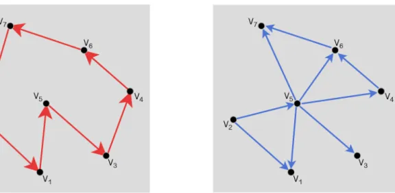
Figure 1.7 A set of vertices V = (V1, . . . , V7), a cyclic digraph (E1, V) pictured left, and an acyclic digraph (E2, V) pictured right.
If the above properties hold, we say that (X,R) is a totally ordered set.
For instance, the set of all real numbers Ris considered totally ordered by the operator “less than or equal to,” since it adheres to the above relations. However, the same cannot be said about R2, nor Z×Z. Thus, there is not a total canonical order of the pixels of an image. To
this end, we define a partial order as follows:
Definition 1.5.2. LetX be a set of elements. A binary relation≺onX is said to be apartial order if and only if
1. For any a∈X,a≺a. (reflexivity)
2. For any a, b∈X, ifa≺band b≺a, then a=b. (antisymmetry)
3. For any a, b, c∈X, if a≺b andb≺c, thena≺c. (transitivity)
If the above properties hold, we say that (X,≺) is a partially ordered set or poset.
A good example of a poset is the set of all subsets of a given set, with the relation being set inclusion. Note that not every two subsets are related by inclusion. This is the main difference between a partial order and a total order.
LetV = (v1, v2, . . . , vk)be a set of vertices, and letE ={(i, j)|vi, vj ∈V and (i,j) is an edge
with tail oniand head onj} be the set of directed edges between vertices inV. We define the set (V, E) as a directed graph, or adigraph. Formally, a digraph (V, E1) is consideredcyclic if every edge{(i1, j1),(i2, j2), . . . ,(in, jn)}=E satisfiesjk=ik+1for everyk∈ {1, . . . , n−1}and
jn =i1. Therefore, a digraph (V, E2) is considered acyclic when there exists no sequence ofr edges((i1, j1),(i2, j2), . . . ,(ir, jr))satisfyingjl=il+1, l∈ {1, . . . , r−1}, andjr=i1. Figure1.7 illustrates two examples of a cyclic digraph and an acyclic digraph. Every edge in a cyclic digraph points in the same direction. In this sense, it is possible to choose any vertex vi and
travel across a finite number of edges to reachvi again. Conversely, an acyclic digraph contains
no cyclic sub-digraphs. Note that a digraph need not fall into one of these two categories. We now apply this graph-theoretic model and the notion of a partially ordered set to an image. Let(V, E)be an acyclic digraph, whereV ={v1, v2, . . . , vk}is a finite set. We construct
a poset corresponding to this digraph as follows:
vi ≺vi, for i= 1, . . . , k
vi ≺vj, if there exists a directed path from vi to vj in(V, E).
(1.27)
Conversely, given a finite poset(V,≺), a corresponding acyclic digraph can be created by defin-ing the set of edges E as follows:
(vi, vj)∈E if and only if vi≺vj and there does not exist a third
elementvz 6=vi, vj such thatvi ≺vz ≺vj.
(1.28)
We see that the correspondence in (1.28) is many-to-one. There exist multiple acyclic
digraphs that can correspond with the same poset. However, if we start with an acyclic digraph as in (1.27), the corresponding poset is unique. We use this to describe the spatial relations
between pixels in an image. We now give four definitions that lay the graph-theoretic foundation for POMMs.
Definition 1.5.3. Let(V,≺) be the poset associated with the acyclic digraph of (V, E). For any B ∈V, thecone of B is the set B ={C ∈V |C≺B, C 6=B}.
Definition 1.5.4. For anyB∈V, theadjacent lower neighbors of B are those elementsC∈V
such that (C, B) is a directed edge in a graph (V, E). Formally, adj≺B = {C | (C, B) is a directed edge inE}.
Definition 1.5.5. An element B ∈V is aminimal element if there is no element C∈V such thatC ≺B.
Definition 1.5.6. Let L0 be the set of minimal elements in the poset. The partially ordered Markov model (POMM) is defined as follows: LetB ∈V where(V, E)is a finite acyclic digraph of random variables and(V,≺) is its corresponding poset. Describe the set of random variables not related to B by YB ={C ∈V |B andC are not related}. Then(V,≺) is called a partially
ordered Markov model (POMM) if for anyB ∈V\L0 and any subsetUB ⊂YB, we have
P(B|cone B, UB) =P(B|adj≺B). (1.29)
We explain how POMMs are used for the purposes of steganalysis in Chapter 4.
1.6 Pseudo-random number generators
Pseudo-random number generators are deterministic algorithms that generate a long se-quence of digits that statistically resemble a string of truly randomized digits. The digit pro-duced by a pseudo-random number generator is determined by the state of the generator, or the input given to the generator function. The state of the generator changes after a digit is produced. The initial state of a generator is based on aseedvalue supplied by the user, and this state is referred to theseed state. The set of all possible seed values is called the seed domain.
This is where the “pseudo-random" part of the name comes from; given a specific state, a random number generator will always produce the same digit. In this sense, a pseudo-random number generator is never truly pseudo-random. It is important to note that all pseudo-pseudo-random number generators are periodic. Eventually, the sequence will repeat itself. If the state of the generator containsnbits, then the period of the pseudo-random sequence has a maximal period of 2n bits.
There are ways to generate truly random sequences of numbers, but they are all hardware-based. Some examples include measuring the elapsed time between emissions of particles in
radioactive decay or thermal noise from a resistor. However, it is impractical to use these meth-ods for modern applications that require a random string of digits. Many different algorithms exist for computing pseudo-random sequences and they typically leverage a computationally difficult problem, such as the factorization of large integers or the discrete logarithm problem, to ensure the security of the generator’s state. This makes pseudo-random number generators well-suited for cryptography since the secret state can act as a shared key between two parties. A pseudo-random number generator is considered cryptographically secure if it satisfies the following properties:
1. Givenk digits of a pseudo-random sequence, there is no polynomial-time algorithm that can predict the(k+ 1)th digit of the sequence, and
2. Should the state of the generator become compromised, there is no polynomial-time algo-rithm that can reproduce the string of pseudo-random digits prior to the state. In other words, the previous states of the generator cannot be determined from the known state.
One example of a cryptographically secure pseudo-random number generator is the Blum-Blum-Shub generator [3]. In the publication where they introduced this generator, they also described the1/P pseudo-random number generator. While the sequences generated by the1/P generator share characteristics with a truly random sequence, it is shown that the 1/P generator is not cryptographically secure. Given a small string of digits from the pseudo-random sequence, it is possible to determine the state of the generator which allows an attacker to extend the sequence both forwards and backwards, violating both definitions of a cryptographically secure generator. However, the predictability of the generator is a desirable characteristic for the psteg algorithm, which we will illustrate later. We explore the 1/P generator in the next section.
1.6.1 1/P pseudo-random number generator
Fix an integer baseb >1, and letΣ ={0,1,· · · , b−1}be the set of base-bdigits. We define
Σ∞as the set of all infinite sequences of base-bdigits. LetP={P ∈Z|P >1,gcd(P, b) = 1}be the set of integers relatively prime withb such thatb is a primitive root moduloP. Note that
for anyP ∈P, bis a generator for the unique cyclic group of unitsZ∗P.Let the seed domain be
X={(P, r)|P ∈P, r∈Z∗
P}.
We define the1/P generatorG:X→Σ∞; (P, r)7→G(P, r)as a function that takes the seed
(P, r)from the seed domainX and maps it to the infinite sequence ofb-ary digitsG(P, r)∈Σ∞, whereG(P, r)is the expansion ofr/P baseb. The pseudo-random sequenceG(P, r)has period
P−1.
For example, fix b= 10, and let P = 17 and r = 1. Then G(17,1) is the pseudo-random sequence of base-10 digits q = (0,5,8,8,2,3,· · ·). This can be verified by evaluating 1/17 = 0.058823· · · and lettingq0 = 0, q1 = 5, q2= 8,and so on.
The pseudo-random sequence G(P, r0) can started at any position in the sequence by ini-tializing the generator with seed state(P, ri), where
ri=bir0 (modP) (1.30)
Proof. Let(P, r0)be the seed of the 1/P generatorG, and let the sequenceG(P, r0) = (q0, q1, q2. . .) be the sequence of base-b digits generated byG(P, r0).
r0 P = 0.q0q1q2 · · · (1.31) bir 0 P =q0q1q2· · ·qi−1.qiqi+1qi+2 · · · (1.32) =q0q1q2· · ·qi−1+ 0.qiqi+1qi+2 · · · (1.33) Letk=q0q1q2· · ·qi−1 ∈N. Then bir0 P =k+ 0.qiqi+1qi+2 · · · (1.34) bir0 =P k+P·0.qiqi+1qi+2 · · · (1.35) bir0−P k=P ·0.qiqi+1qi+2 · · · (1.36) bir0 (modP) =P ·0.qiqi+1qi+2 · · · (1.37) bir0 (modP) P = 0.qiqi+1qi+2 · · · (1.38)
Letri=bir0 (modP). Then
ri
P = 0.qiqi+1qi+2 · · · (1.39)
1.6.2 Predictability of 1/P
The state of the1/P generator can be quickly calculated given only a small number of digits from the pseudo-random sequence [3]. This is illustrated by continued fractions. By LeVeque [13], the continued fraction expansion of a real numberx has a convergentp/q if and only if
x−p q < 1 2q2. (1.40)
Let0< m < P be a natural number and letk∈N. By (1.31), (1.33), and (1.39), we have
bkrm P =qm· · ·qm+k−1+ rm+k P (1.41) rm P = qm· · ·qm+k−1 bk + rm+k P · 1 bk (1.42) qm· · ·qm+k−1 bk − rm P = rm+k P · 1 bk (1.43) qm· · ·qm+k−1 bk − rm P < 1 bk, (1.44)
where the inequality stems from the fact that rm+k < P by definition. By (1.40), if 1/bk < 1/2P2, then rm/P is a convergent of the continued fraction expansion of qm· · ·qm+k−1/bk. Thus, ifk≥logb(2P2) digits of a pseudo-random sequence generated by the1/P generator are known, then bothrm and P can be determined. The sequence can be expanded both forwards
and backwards from (1.30) by letting
rm+1 =brm (mod P) (1.45)
and
rm−1 =b−1rm (modP), (1.46)
whereb−1 is the multiplicative inverse of bmodulo P.
1.7 The psteg algorithm
The idea behind the psteg algorithm is best illustrated by example. Suppose that Alice wants to embed a payloadm= 00101110into a spatial domain, 8-bit, grayscale cover imagex
Table 1.3 The number of changes ncrequired to embedm intoˆx1 and xˆ2. i= 1 i= 2 i= 3 i= 4 i= 5 i= 6 i= 7 i= 8 nc mi 0 0 1 0 1 1 1 0 LSB(ˆx1 i) 0 1 0 0 0 1 1 1 4 LSB(ˆx2 i) 0 0 1 0 1 1 1 0 0 defined as x={155,178,83,140,33,77,122,234}. (1.47) Furthermore, suppose that she wants to use LSB replacement as her embedding algorithm. Alice chooses her stego key to be k1 and uses it to generate a random permutation σ1, which she uses to permute x.
σ1(x) = ˆx1={122,83,234,178,140,155,77,33} (1.48)
She replaces the LSBs of the pixels of xˆ1 withmto create yˆ1.
ˆ
y1 ={122,82,235,178,141,155,77,32} (1.49) During the embedding process, Alice had to change the LSB of four pixels (boldfaced above) to embed eight bits of information. The embedding operation had an embedding rate of 1 bit-per-pixel and an efficiency of 8/4 = 2 bits embedded per change, which matches the expected embedding efficiency of the LSB replacement.
Suppose that Alice embeds the same payload into the same image, except that this time she uses k2 to generate a different random permutationσ2 which she uses to permutex.
σ2(x) = ˆx2={234,140,33,122,77,155,83,178} (1.50)
Alice replaces LSBs of the pixels in ˆx2 withmto create yˆ2.
ˆ
y2 ={234,140,33,122,77,155,83,178}. (1.51) Notice that Alice made no changes to the LSBs of xˆ2 to embed the payload m. The embedding rate is still 1 bit-per-pixel, but the embedding efficiency is8/0 =∞. In other words,
as well as first-order and second-order feature-based attacks. It is also safe against brute force stego key searches since one byte of information doesn’t make any more “sense" than another byte. So how many keys do we expect that needs Alice to try until she finds such a stego key? For a given cover imagexwithntotalembeddable locations, let the number of even-valued pixels in x be denoted by neven and the number of odd-valued pixels be denoted by nodd. Let the payloadmcontainltotal ≤ntotalbits, and let the number of even and odd bits inmbe denoted
by leven and lodd, respectively. Then the number of golden permutations, given by
neven!
(neven−leven)!
· nodd!
(nodd−lodd)!
·(ntotal−ltotal)!, (1.52)
is the number of permutations ofx such that the firstltotal LSBs ofx match the payload m. In the example given above, Alice’s cover imagexhasntotal= 8pixels withneven=nodd= 4, and her payloadmhas length ltotal= 8 withleven=lodd= 4. By (1.52), the number of golden permutations is
4! (4−4)!·
4!
(4−4)!·(8−8)! = 4!·4!·1! = 576, (1.53)
The number of all possible permutations of an image with eight pixels is 8! = 40320. Since we assume that the pseudo-random number generator used to generate the permutations is cryp-tographically secure, we can assume that the generated permutations are uniformly distributed across the stego key space K(x). Thus, the probability that a given stego key k is a golden stego key is576/40320≈0.014.
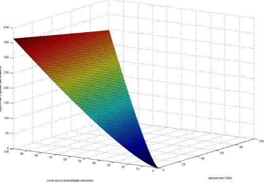
However, the difficulty of finding a golden stego key increases with the sizes of the payload and cover image, as is shown in (Figure 1.8). Consider the set of 512-by-512 8-bit grayscale
cover images X = {0, . . . ,255}512×512. For any given cover image x ∈ X, there exist (5122)! total possible permutations of the image. Assume that the parity distribution on x is equal, so that neven = nodd = ntotal/2 = (5122)/2 = 131072. Furthermore, assume that m is an encrypted payload with equal parity distribution (leven=lodd =ltotal/2, whereltotal is an even number). Then by (1.52), the number of golden permutations is
131072! (131072−ltotal/2)!
2
Figure 1.8 The logarithm of the number of golden permutations as a function of cover size n
and payload sizel.
If the payload size is only eight bits as it was in the first example of this section, then the probability that Alice chooses a golden key k is merely ≈ 1/256. However, a more realistic payload of 2000 bits gives a probability of ≈1/10602. With this in mind, a brute force search is not a feasible method for attempting to find a golden stego key in a practical-use scenario.
It should be noted that ifltotal= 0, the number of golden permutations isntotal!, the number of all possible permutations. Ifltotal=ntotaland they both have an equal parity distribution, the number of golden permutations is((ntotal/2)!)2, and ((ntotal/2)!)2 < ntotal!for all n. It should also be noted that for a given ltotal, the probability that a randomly generated permutation is also a golden permutation approaches 1/2ltotal asn
total goes to infinity.
As opposed to finding a golden stego key by brute force, perhaps we might be able to construct such a key. While the golden permutations are trivial to generate, the difficulty lies in finding a stego key that initializes a pseudo-random number generator to create the permutation. Suppose that we know a pseudo-random sequence from a generator that creates a
golden permutation. If the pseudo-random number generator is cryptographically secure, then by definition, it is impossible to find (in polynomial time) the state of the generator based only upon knowledge of the pseudo-random sequence.
Consider using the 1/P generator to create the permutation. We have established that the entirety of the pseudo-random sequence can be generated both forwards and backwards using only a small sample of the sequence. Furthermore, the state of the generator can be ascertained. In our case, this is equivalent to finding a stego key that generates a golden permutation. Recall from (1.44) that if we know k ≥ logb(2P2) base-b digits of a 1/P generated sequence
G(P, r) = (q1, q2, . . . , qk), then we can determine both r and P. Let x ∈ X = {0, . . . , b}c be
an b-ary grayscale cover image with c pixels, and let m be a bitstring payload of size k < c. Choose a sequence of distinct elementss= (x1, x2, . . . , xk)fromxsuch thatLSB(xi) =mi for
0< i < k. If we find a convergent Ai/Bi of q1q2· · ·qk/bk such that G(Bi, Ai) generatess, then
(Bi, Ai) is a stego key that generates a golden permutation of xfor the payload m.
While this might initially seem like a straightforward solution to the problem at hand, several other problems exist that preclude the feasibility of this in a practical-use scenario. The computational complexity involved in computing such convergents is high. Since the stego key is dually dependent on both the cover object and the payload, it is impossible to pre-arrange a key between the two parties at either end of the steganographic channel. Even if side communication is allowed between them, the size of the stego key (P, r) will usually be exponentially larger than that of the hidden message. At this point, it becomes trivial to encrypt and send the stego key when the payload itself could instead be encrypted and transmitted. goo Instead of finding a golden permutation, we propose to use the 1/P generator to improve the embedding efficiency of the LSB replacement algorithm. The steganographer first chooses a prime stego key P. The payload and the elements of the cover image are divided into partitions. For each partition, we exhaustively search for a permutation generated by 1/P that best matches our payload partition. The values of r and the baseb are stored in the header of the cover image partition, and the values that don’t match are altered so that they match the payload. The algorithm is explained in greater detail in Chapter 3.
CHAPTER 2. STEGANOGRAPHIC ALGORITHMS
While steganography has been in practice since the times of Ancient Greece (the etymology of the word "steganography" having Greek roots, literally meaning "covered writing"), modern steganography has been around since the advent of the personal computer in the mid-1980s. The practice of open security is generally accepted by the steganography community, in which the details of a proposed stegosystem are published for the entire community to scrutinize. This is in direct contrast to the practice of security through obscurity, or keeping the details of the stegosystem secret. In 1883, Auguste Kerckhoffs created six basic principles to which all cryptosystems should adhere. Many of his principles have been considered archaic since advent of computers, but his second principle (now referred to simply as Kerckhoff’s principle) is still applicable and is widely regarded as a strong guideline to consider during the design of a cryptosystem. Paraphrased, it states that the security of a stegosystem should rely solely in the secrecy of the key; we assume that an attacker knows the details of the stegosystem’s innards. The Enigma machine is a classic example of a cryptosystem practicing security through obscurity. While the system was very robust to cryptanalysis, knowledge of the machine’s inner workings led to the deciphering of many messages encrypted with Enigma. Note that Kerckhoff’s principle does not advocate open security. The principle simply requires that a system should remain secure despite knowledge of the system’s workings.
Although many steganographic embedding algorithms have been proposed, very few have been shown to be secure when embedding large payloads. A digital image stegosystem is typically specialized toward embedding in either the spatial domain or the frequency domain, but not both. This is due to the fact that embedding algorithms are usually designed to preserve the statistical model of the cover image. If a stegosystem tries to preserve the statistical model of quantized AC coefficients in the frequency domain, it doesn’t make sense to try to apply the
stegosystem to the spatial domain. While there currently exist secure stegosystems that embed into the spatial domain, the popularity and prevalence of the JPEG image format has directed the focus of many modern stegosystems towards embedding in the frequency domain. We have shown that it is possible to transform the frequency data into spatial data, but it is pointless to embed information here if the image will be transformed back into the frequency domain since the JPEG format loses some spatial data during the quantization step. Thus, embedding directly into the frequency domain is the most reliable method of steganography using JPEG images.
2.1 F5 and nsF5
In [21], Westfeld introduced the F5 algorithm. A total of three algorithms are detailed, and each successive algorithm builds on the previous one. The first algorithm, F3, introduces the novel concept of decrementing the absolute value of nonzero quantized AC coefficients as opposed to strictly overwriting the LSB. It avoids embedding into zero quantized AC coefficients as the recipient of the stego image would have no way of differentiating a naturally occurring0
from a 0 created by the embedding operation. This preserves the symmetry of the histogram of quantized AC coefficients reflected about the 0 coefficient, but still produces an abnormal histogram due to shrinkage. The term shrinkage is used to describe the phenomena of an quantized AC coefficient±1decreasing its absolute value to 0. In such a case, the same payload bit is carried over to the next quantized AC coefficient. This process is repeated until the bit is embedded without changing an quantized AC coefficient from ±1 to 0. As a result, the resultant histogram of a stego image embedded with F3 shows that the image contains more even coefficients than is to be expected.
The second algorithm, F4, alleviates this issue by inverting the steganographic value of negative quantized AC coefficients. In this sense, an quantized AC value of −1 becomes a steganographic0. While shrinkage still occurs, it is less frequent and produces a more natural histogram than F3. The final algorithm, F5, introduces two new concepts to F4. Permutative straddling is used as a linear time complexity model for spreading the payload evenly across the cover image. Matrix encoding, first proposed by Crandall [5], is integrated into the embedding
Table 2.1 The truth table for the "exclusive or" (⊕) operation.
0⊕0 = 0
0⊕1 = 1
1⊕0 = 1
1⊕1 = 0
process to maximize the embedding efficiency of the algorithm. As the ratio of payload bits per nonzero quantized AC coefficients decreases, the embedding efficiency increases. Westfeld provides the following example to demonstrate the simplest, and least efficient, method of matrix encoding.
Suppose that we want to embed two bits x1, x2 into three LSBs of a cover image a1, a2, a3. Consider the following possible scenarios:
x1 =a1⊕a3, x2=a2⊕a3 =⇒ change nothing (2.1)
x1 6=a1⊕a3, x2=a2⊕a3 =⇒ change a1 (2.2)
x1 =a1⊕a3, x2=6 a2⊕a3 =⇒ change a2 (2.3)
x1 6=a1⊕a3, x2=6 a2⊕a3 =⇒ change a3, (2.4) where the operation⊕is the exclusive-or operation defined in Table 2.1. We are able to embed
two bits of information into three pixels, but we only need to change one pixel value. In this sense, we measure the efficiency of the F5 algorithm as the embedding rate per expected value of pixel change. In general, to embedkbits inton= 2k−1elements of a cover, the embedding
efficiency is given by
e= 2
k
2k−1 ·k. (2.5)
The efficiency of the algorithm strictly increases with increasing k. For a given binary payload
mand cover imagexwithnx elements, the maximum value ofkis the smallest natural number
a∈Nsatisfying the inequality
a 2a−1 >
log2(m)
nx
. (2.6)
In 2007, Fridrich et. al. proposed a solution to the problem of shrinkage by incorporating wet paper codes [10] into F5, and they call the revised algorithm nsF5 (no shrinkage). Wet