Multicut Algorithms for Neurite Segmentation

(1)

DISSERTATION

submitted

to the

Combined Faculty for the Natural Sciences and

Mathematics

of

Heidelberg University, Germany

for the degree of

Doctor of Natural Sciences

Put forward by MSc Thorsten Beier Born in Heidelberg, Germany Oral examination:

(2)

(3)

Multicut Algorithms for Neurite Segmentation

Thorsten Beier

(4)

(5)

Abstract

Correlation clustering, or multicut partitioning is widely used for image segmentation and graph partitioning. Given an undirected edge weighted graph with positive and negative weights, correlation clustering partitions the graph such that the sum of cut edge weights is minimized. Since the optimal number of clusters is automatically chosen, multicut partitioning is well suited for clustering neural structures in EM connectomics datasets where the optimal number of clusters is unknown a-priori. Due to the NP-hardness of optimizing the multicut objective, exact solvers do not scale and approximative solvers often give unsatisfactory results.

In chapter 2 we investigate scalable methods for correlation clustering. To this end we define fusion moves for the multicut objective function which iteratively fuses

the current and a proposed partitioning and monotonously improves the partitioning. Fusion moves scale to larger datasets, give near optimal solutions and at the same time show state of the art anytime performance.

In chapter 3 we generalize the fusion moves frameworks for the lifted multicut

ob-jective, a generalization of the multicut objective which can penalize or reward all decompositions of a graph for which any given pair of nodes are in distinct compo-nents. The proposed framework scales well to large datasets and has a cutting edge anytime performance.

In chapter 4we propose a framework for automatic segmentation of neural structures in 3D EM connectomics data where a membrane probability is predicted for each pixel with a neural network and superpixels are computed based on this probability map. Finally the superpixels are merged to neurites using the techniques described in chapter 3. The proposed pipeline is validated with an extensive set of experiments and a detailed lesion study. This work substantially narrows the accuracy gap between humans and computers for neurite segmentation.

In chapter 5 we summarize the software written for this thesis. The provided imple-mentations for algorithms and techniques described in chapters2to4and many other algorithms resulted in a software library for graph partitioning, image segmentation and discrete optimization.

(6)

Zusammenfassung

Correlation Clustering oder Multicut Partitionierung ist eine weit verbreitete Technik zur Bildsegmentierung oder Graphpartitionierung. Correlation Clustering partitioniert einen kantengewichteten Graph mit positiv und negativ gewichteten Kanten sodass die Summe der Kantengewichte der geschnittenen Kanten minimiert wird. Da die optimale Anzahl der Kluster automatisch ausgewählt wird, ist die Multicut Paritionierung gut geeignet um neuronale Strukturen in sogenannten EM-Konnektom Datensätzen zu segmentieren, da dort die optimale Anzahl von Klustern nicht a-priori bekannt ist. Da es NP-hart ist die Multicut Zielfunktion zu optimieren skalieren exakte Algorithmen nicht und approximative Verfahren geben schlechte Resultate.

In Kapitel 2 untersuchen wir skalierende Methoden für Correlation Clustering. Wir definieren Fusion Moves für die Multicut Zielfunktion. Fusion Moves ist ein iteratives

Verfahren das die momentane Partitionierung mit einer Kandidatenpartitionierung fusioniert und so monoton die Partitonierung verbessert. Fusion Moves skaliern zu großen Datensätzen, geben nahezu optimale Lösungen und haben eine gute Perfor-mance selbst wenn sie vor der Terminierung unterbrochen werden.

In Kapitel3generalisieren wirFusion Moves für die Lifted Multicut Zielfunktion, eine

Generalisierung der Multicut Zielfunktion welche alle Partitionierungen eines Graphes belohnen oder bestrafen kann in der ein beliebiges paar von Knoten in verschiedenen Klustern ist. Die vorgeschlagenen Methoden skalieren gut und haben ein guten Per-formance selbst wenn sie vor der Terminierung unterbrochen werden.

In Kapitel 4 wird ein Framework zur automatischen Segmentierung von neuronalen Strukturen in 3D EM Daten vorgestellt. Startend von einer mit einem neuronalen Netz gelernten pixelweisen Membranwahrscheinlichkeit wird eine Superpixel Überseg-mentierung erzeugt. Die Superpixel werden mit den in Kapiteln 2 und 3 vorgeschla-genen Methoden zu Neuronen zusammengefügt. Das vorgeschlagene Framework wird durch umfangreiche Experimente und eine detailreiche Läsion Studien validiert. Der Qualitätsunterschied zwischen menschlich erzeugten Segmentierungen und automa-tisch erzeugten Segmentierungen wurde durch das vorgeschlagene Framework deutlich verringert.

In Kapitel5wird die für diese Thesis geschriebene Software zusammengefasst. Die be-reitgestellten Implementierungen für die Algorithmen aus Kapitel2-4und viele andere Algorithmen resultierten in einer Software Bibliothek zur Graph Partitionierung und Bildsegmentierung.

(7)

Acknowledgments

First, I like to thank Professor Fred Hamprecht for being the Supervisor for this thesis. I have been working in his research group Image Analysis and Learning for

almost a decade. Since I joined the group as bachelor student, it has always been a pleasure to collaborate with so many friendly, intelligent and helpful people. I like to thank Bjoern Andres and Jörg Kappes for introducing me to the field of discrete optimization and many hours of fruitful discussions about algorithms and software. I like to thank Ullrich Köthe for many fruitful discussion about image segmentation, algorithms and software in general. I like to thank Thorben Kroeger, Niko Krasowki, Anna Kreshuk and Constantin Pape for our strong collaboration and joint work on automatic segmentation for 3D-EM Data. In particular I like to thank Constantin Pape for the many hours of work he invested in joint research papers and software projects. I had many enjoyable moments with Christoph Straehle and Luca Fiasch and Sven Wanner outside of the building. I enjoyed the special humor of Philipp Hanslovsky and Robert Walecki very much. I enjoyed many cups of coffees with Steffen Wolf, Lorenzo Cerrone, Constantin Pape, Phillip Schmidt, Peter Neigel, Christoph Straehle, Nasim Rahaman and Anna Kreshuk where we hand many enjoyable discussions. A special thanks to Barbara Werner for all her incredible work.

(8)

(9)

1 Introduction

1.1 Image Segmentation

Image segmentation is arguably the most important task in computer vision. It is the fundamental building block for many application and therefore fast and accurate segmentations algorithms are needed. Many flavors of segmentation exists: i) Class-level segmentation where each pixel is assigned to a single class from a discrete set

as {sky,car,road,person}. ii) Instance-level segmentation where each pixel is not

only assigned to a single class from a discrete set as {sky,car,road,person} but also a unique instance id, e.g. person-1, person-2, car-1. The number of instances per

class is not known beforehand in this setting and iii) One-Class-Instance-Level as a

special case ofInstance-level segmentation with only a single class. Again, the number

of instances is not known in advance. An example for this kind of segmentation is given in fig. 1.1 where each pixel is assigned to the id of the corresponding neural process, e.g.neuron-1, neuron-2, neuron-3.

In this thesis we will focus on the latter one, One-Class-Instance-Level segmentation

for connectomics as described in the following section.

1.2 Segmentation for Connectomics

To understand how the brain is working neuroscientists are acquiring large volumes of electron microscopy (EM) images of the brain of animals with the aim of analyzing the neural circuit connectivity of the brain. This circuit formed by neurons which are connected via synapses is the so calledconnectome.Connectomics is the field of science

acquiring and studying connectomes. The connectome can be acquired by sequencing

techniques [149] or by segmentation based approaches. Here, we only discuss the latter one. Given a segmentation of the neurons in EM volumes, synapses and their synaptic partners need to be detected [88,90,128] to form the graph known as connectome. In this thesis we will focus on automated segmentation of neurons. Detection of synapses and their synaptic partners is beyond the scope of this thesis.

(14)

z

(a) Stack of raw data and corresponding segmentation

(b) 3D visualization of result from a multicut approach [9]

Figure 1.1: Figure 1.1a: A stack of 2×2 microns slices of from a transmission Electron Mi-croscopy (ssTEM) data set of the Drosophila first instar larva ventral nerve cord (VNC) with a resolution of × × nm/pixel [19] and a manual created

(15)

Despite impressive progress in collaborative annotation [79], the sheer size of these volumes make manual analysis infeasible. To handle large whole-brain datasets au-tomated segmentation is needed. In chapters 4 and 5 we present algorithms and a software package to automatically segment such data sets with low error rates. The al-gorithms are based based on the multicut [8,68] and lifted multicut [7,78] formulation which we will briefly described in the following sections.

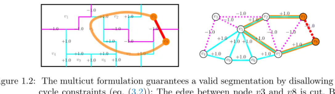
1.2.1 Multicut −1.0 −1.0 +1.0 −1.0 −1.0 −1.0 +1.0 −1.0 +1.0 +1.0 +1.0 +1.0 +1.0 +1.0 +1.0 +1.0 v1 v2 v3 v4 v5 v6 v7 v8 v9 v1 v2 v3 v4 v5 v6 v7 v8 v9 −1.0 −1.0 −1.0 +1.0 +1.0 −1.0 −1.0 −1.0 +1.0 +1.0 +1.0+1.0 +1.0 +1.0 +1.0 +1.0 v3 v8 −1.0 v3 v8

Figure 1.2: The multicut formulation guarantees a valid segmentation by disallowing violated cycle constraints (eq. (3.2)): The edge between node v3 andv8 is cut. But there is a path of uncut edge connecting v3 and v8 depicted in orange. The multicut objective can be optimized by adding violated constraints to an ILP in a cutting plane fashion [8, 68].

The multicut [25] and lifted multicut problem [7,78] have become increasingly popular in the recent years [8,23,26,27,29,68,81,83,92,99,112,113,135,146,147]. Given a graph G = (V, E) with edge weights w : E → _R the minimum multicut minimizes the sum of weights between clusters. Formally the minimum multicut is defined as: y∗ = arg min y∈{0,1}E X e∈E weye (1.1) subject to ∀C∈cycles(G) ∀e∈C: ye≤ X e0_∈_C_\{_e_} ye0 (1.2) | {z }

Ensures valid segmentations without dangling edges as illustrated in fig.1.2

Multicuts have several advantages compared to traditional algorithms operating on a weighted graph:

i) Graph-cuts [85] and normalized cuts [123] can only model positive weight (attrac-tion) and ii) suffer from a shrinking bias [45,141] while the multicut formulation allows

(16)

for positive (attraction) and negative (repulsion) edge weights and does not suffer from a shrinking bias. iii) While QPBO [118] and multi-label variants [84] can handle posi-tive and negaposi-tive weights, the maximum number of classes/ clusters needs to be fixed beforehand. The multicut approach does not need a specified number clusters, the optimal number of classes is implicitly choose by the optimal solution.

On the down-side, solving the multicut problem is in general NP-hard. Since the set of constraints in eq. (1.2) is of exponential size any exact solver will have scalability issues.

A detailed review of the multicut objective and optimizer is given in sections 2.1.2

and 3.2.1.

1.2.2 Lifted Multicut

The minimum lifted multicut problem [7,78] is an optimization problem whose feasible solutions are decompositions of a graph. The objective function can penalize or reward all decompositions for which any given pair of nodes are in distinct components. Given a graph G = (V, E) and a larger graphG0 = (V, E0) with E ⊆E0 and edge weights w :E0 → _R, where the weights penalize or reward precisely the decompositions of G

for which the nodes v andw are in distinct components. The lifted multicut problem

is defined as: y∗= arg min y∈{0,1}E0 X e∈E0 ceye (1.3) subject to ∀Y ∈cycles(G) ∀e∈Y : ye≤ X e0_∈_Y_\{_e_} ye0 (1.4) | {z }

Ensures valid segmentations without dangling edges as depicted in fig.1.2

∀vw∈E0\E ∀P ∈vw-paths(G) : yvw ≤ X

e∈P

ye (1.5)

| {z }

If additional edges wvis cut, ensure that no path of uncut edges between u and v inGexists ∀vw∈E0\E ∀C∈vw-cuts(G) : 1−xvw≤

X

e∈C

(1−ye) (1.6)

(17)

Like the multicut, solving the lifted multicut problem is in general NP-hard. A detailed review of the lifted multicut objective and optimizer is given in sections3.1and3.2.2. In chapters 2 and 3 we will propose a fusion moves based algorithm for optimizing

the multicut and lifted multicut algorithm respectively. The concept of fusion moves

is described in the following section.

1.3 Fusion Moves

For energy minimization problemsfusion moveshave become increasingly popular [66,

96,102,148]. The fusion move is an algorithm to combine pairs of suboptimal solutions using graph-cut [85] or QPBO [118]. For many large scale computer vision applications fusion moves yield good approximations with state of the art anytime performance [66]. Fusion moves can be described as a class of constrained search algorithms. They consist of two procedures. The first procedure is proposal generation that computes a feasible solution in a possible randomized randomized fashion. Second is fusion where the

proposal is combined with the current best solution. This can be formalized in the following way: Given pairwise MRFs / CRFs in the form of

y∗ = arg min y∈Y X u∈V Uu(yu) + X uv∈E Vuv(yu, yv) (1.7)

and pair of labels ya, yb∈Y (also called proposals), the fusion move is defined as:

y∗ = arg min y∈Y X u∈V Uu(yu) + X uv∈E Vuv(yu, yv) (1.8) s.t. xi ∈ {yia, ybi} ∀yi ∈Y

Equation (1.8) can be optimized with graph-cut [85] or QPBO [118]. We will use

F MM RF to refer to eq. (1.8). The proposals themselves can be computed by a domain

specific method most suitable for the given task.

1.4 Contribution and Overview of this Thesis

The chapters are structured in the following way: In chapter 2 we generalize fusion moves [96] for the minimum multicut objective: Instead of directly optimizing the multicut objective, we iterativelyfuse a current best solution with candidate solutions

(18)

such that the best energy is improved. The fusion procedure in itself is again a

min-imum multicut optimization problem with additional must-link constraints. We show how to formulate this as anunconstrained1 minimum multicut problem with a smaller

number of variables and constraints. We investigate how to generate high quality can-didate solutions in an efficient manner. To this end we define two cancan-didate solution generators based on the watershed transform and agglomerative clustering in conjunc-tion with perturbed edge weights. We use these generators in an iterative manner and fuse the generated solutions with the current best solution. Based on this we derive a set of scalable algorithms with state-of-the art anytime performance yielding solutions close to global optimality.

In chapter3we generalize thefusion movesframework [96] and the algorithm presented

in chapter 2 to the minimum lifted multicut problem [7, 78]: Again, we iteratively

fuse a current best solution with candidate solutions to minimize the minimum lifted

multicut objective function. Thefusionprocedure in itself is a minimum lifted multicut

problem with additional must-link constraints. We show how to reformulate this as an unconstrained minimum lifted multicut problem2_{. We propose efficient candidate}

solution generators to quickly generate diverse high quality solutions which are fused

with the current best solution. Based on this, we derived a set of scalable algorithms with state-of-the art anytime performance.

In chapter 4, we apply the algorithms proposed in chapters 2and 3to the problem of segmentation of neural structures in EM data. We propose a state-of-the art pipeline and validate every step in the pipeline with extensive experiments. We predict the membrane probability for each pixel using a convolutional neural network. We use the watershed transform on a distance transform height map based on the membrane probabilities to generate superpixels for each 2D slice of the 3D stack. Finally, we use a Random Forest to learn and predict which pairs of superpixels should be merged and jointly optimize this with the multicut and lifted multicut algorithms proposed in chapter 2 and chapter3 respectively.

In chapter5we discuss the software implemented to conduct the experiments through-out this thesis. We provide implementations for algorithms and techniques described in chapters 2 to4 resulting in a C++ software framework for graph partitioning and image segmentation. Not only do we provide fast and readable modern C++code, but

also a fully functional Python API.

In chapter 6 is a enumeration of all peer reviewed publication where I was author or co-author. Chapters2to4are based on publications [26,27,30] in top ranked venues.

(19)

2 Fusion Moves for Multicut Partitioning

Correlation clustering, or multicut partitioning, is widely used in image segmentation for partitioning an undirected graph or image with positive and negative edge weights such that the sum of cut edge weights is minimized. Due to its NP-hardness, exact solvers do not scale and approximative solvers often give unsatisfactory results. We investigate scalable methods for correlation clustering. To this end we define fusion moves for the correlation clustering problem. Our algorithm iteratively fuses the cur-rent and a proposed partitioning which monotonously improves the partitioning and maintains a valid partitioning at all times. Furthermore, it scales to larger datasets, gives near optimal solutions, and at the same time shows a good anytime performance.

2.1 Introduction

Correlation clustering [24], also known as the multicut problem [41] is a basic primitive in computer vision [5,8,9,146] and data mining [16,38,40,120]. See Sec.2.2for its formal definition of clustering the nodes of a graph.

Its merit is, firstly, that it accommodates both positive (attractive)and negative

(re-pulsive) edge weights. This allows doing justice to evidence in the data that two nodes or pixels do not wish or do wish to end up in the same cluster or segment, respectively. Secondly, it does not require a specification of the number of clusters beforehand. In signed social networks, where positive and negative edges encode friend and foe relationships, respectively, correlation clustering is a natural way to detect communi-ties [38, 40]. Correlation clustering can also be used to cluster query refinements in web search [120]. Because social and web-related networks are often huge, heuristic methods, e.g. the PIVOT-algorithm [3], are popular [40].

In computer vision applications, unsupervised image segmentation algorithms often start with an over-segmentation into superpixels (superregions), which are then clus-tered into “perceptually meaningful” regions by correlation clustering. Such an ap-proach has been shown to yield state-of-the-art results on the Berkeley Segmentation Database [5,8,80,146].

While it has a clear mathematical formulation and nice properties, correlation cluster-ing suffers from NP-hardness. Consequently, partition problems on large scale data,

(20)

e.g. huge volume images in computational neuroscience [9] or social networks [97], are

not tractable because reasonable solutions cannot be computed in acceptable time.

2.1.1 Contribution

In this chapter we present novel approaches that are designed for large scale correlation clustering problems. First, we define a novel energy based agglomerative clustering al-gorithm that monotonically increases the energy. With this at hand we show how to improve the anytime performance of Cut, Clue & Cut [29]. Second, we improve the anytime performance of polyhedral multicut methods [71] by more efficient separa-tion procedures. Third, we introduce cluster-fusion moves, which extend the original fusion moves [96] used in supervised segmentation to the unsupervised case and give a polyhedral interpretation of this algorithm. Finally, we propose two versatile pro-posal generators, and evaluate the proposed methods on existing and new benchmark problems. Experiments show that we can improve the computation time by one to two magnitudes without worsening the segmentation quality significantly.

2.1.2 Related Work

A natural approach is to solve the integer linear program (ILP) directly 2.2. To this end, efficient separation procedures have been found [68,71] that allow to iteratively augment the set of constraints until a valid partitioning is found. Alternatively, it is possible to relax the integrality constraints of the ILP formulation [71]. Such an outer relaxation can be iteratively tightened. However, intermediate solutions are fractional and therefore rounding is required to obtain a valid partitioning. For the latter ap-proach column generating methods exist, which work best on planar graphs [146]. Another line of work uses move making algorithms to optimize correlation cluster-ing [23,29,76]. Starting with an initial segmentation, auxiliary max-cut problems are (approximately) solved, such that the segmentation is strictly improved. As shown in [29] only Cut, Glue & Cut (CGC) can deal with large scale problems, but can also suffer from very large auxiliary problems.

Recently, a promising dual decomposition algorithm has been proposed [131] which relies on fast primal heuristics as proposed here for so called rounding.

Outside computer vision, greedy methods [3,48,55,110,126] have been suggested for correlation clustering problems, see [49] for an overview. The PIVOT Algorithm [3] iterates over all nodes in random order. If the node is not assigned it constructs a cluster containing the node and all its unassigned positively linked neighbors. A widely used

(21)

0 1 2

3 4 5

w01 w12

w34 w45

w03 w14 w25

(a)node labels

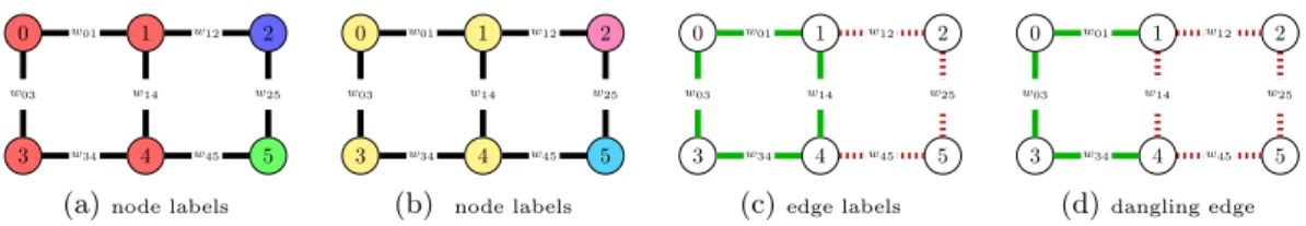
0 1 2 3 4 5 w01 w12 w34 w45 w03 w14 w25 (b) node labels 0 1 2 3 4 5 w01 w12 w34 w45 w03 w14 w25 (c)edge labels 0 1 2 3 4 5 w01 w12 w34 w45 w03 w14 w25 (d)dangling edge Figure 2.1: Representing a clustering by node labels is ambiguous. 2.1a and 2.1b encode the

same partition. Edge labels as in2.1cdo not suffer from such ambiguities, but can havedangling edges as in2.1d. Node1and4are in the same connected component, even tough e14 is cut. This is not a valid partition, and must be ruled out by

constraints. reassigns nodes to clusters.

For energy minimization problems fusion moves have become increasingly popular [66, 96]. For many large scale computer vision applications fusion moves lead to good approximations with state of the art anytime performance [66] Due to the ambiguity of a node-labeling, classical fusion moves [96] cannot be applied directly for correlation clustering ( see fig. 2.3). We will show how to overcome this problem in Sec.2.4.

2.1.3 Outline

In Sec. 2.2 we give a detailed problem definition and introduce the correlation clus-tering objective. Next we give a description of energy based hierarchical clusclus-tering in Sec. 2.3and our proposed correlation clustering fusion moves in Sec.2.4. We evaluate the proposed methods in Sec. 2.5and conclude in Sec. 2.6.

2.2 Notation and Problem Formulation

Let G = (V, E, w) be a weighted graph of nodes V and edges E. The function w : E → R assigns a weight to each edge. We will use we as a shorthand for w(e).

A positive weight expresses the desire that two adjacent nodes should be merged, whereas a negative weight indicates that these nodes should be separated into two distinct regions. A segmentation of the graph Gcan be either given by a node

label-ing l ∈ _N|V| _{or an edge labeling} _y _{∈ {}₀_,₁_}|E|_, _cf_{. Fig.} _2.1_{. An edge labeling is only}

consistent if it does not violate any cycle constraint [41]. We denote the set of all consistent edge labelings by P(G)⊂ {0,1}|E|_{. The convex hull of this set is known as}

(22)

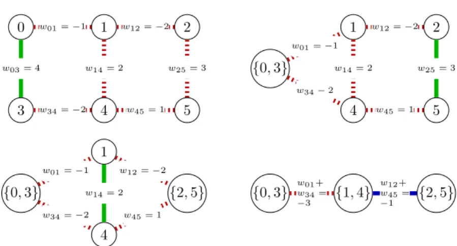
0 1 2 3 4 5 w01=−1 w12=−2 w34=−2 w45= 1 w03= 4 w14= 2 w25= 3 {0,3} 1 2 4 5 w01=−1 w12=−2 w34−2 w45= 1 w14= 2 w25= 3 {0,3} 1 {2,5} 4 w01=−1 w12=−2 w34=−2 w45= 1 w14= 2 {0,3} {1,4} {2,5} w12+ w45= −1 w01+ w34= −3

Figure 2.2: Energy-based Hierarchical clustering can be used to greedily optimize Eq. 2.2. In each step, the two nodes connected via the edge with the highest weight are merged by contracting this edge. (edge to be contracted is shown in green). Due to edge contraction parallel edges can occur, which are merged into single ones, and their weights are summed up. The algorithm terminates when the highest edge weight is smaller or equal to zero (edge shown in blue).

the multicut polytope M C(G) = conv(P(G)). By l(y) we denote some node labeling

for a segmentation given by y.

Given a weighted graph G = (V, E, w) we consider the problem of segmenting G

such that the costs of the edges between distinct segments is minimized. This can be formulated in the node domain by assigning each nodeia label li ∈N

l∗ = arg min

l∈N|V|

X

(i,j)∈E

wij·[li6=lj], (2.1)

or in the edge domain, by labeling each edge eas cutye= 1 or uncut ye= 0

y∗= arg min

y∈P(G)

X

(i,j)∈E

wij·yij. (2.2)

As shown in [71] both problems are equivalent, but formulation 2.1 suffers from am-biguities in the representation, cf. Fig.2.1.

2.3 Energy Based Hierarchical Clustering

(23)

segmenta-in Fig. 2.2). Doing so, parallel edges can occur. In agglomerative clustering, weights of parallel edges are merged into single edges. For image segmentation, the length weighted mean is used to do this update [18].

Because we, contrary to [18], directly work on energies, we use energy based agglom-eration with the following update rule: Whenever there are multiple edges between a pair of nodes, these edges are merged into a single edge and the weights are summed up, since we minimize the sum of the cut edges. We call HC with this update method Energy based Hierarchical Clustering (EHC).

We stop EHC if the highest edge weight is smaller or equal to zero (blue edge in Fig. 2.2). Any further edge contraction does not improve the energies.

Given the intrinsic greediness of hierarchical clustering, we cannot expect EHC to yield optimal solutions in general.

However, EHC is very fast and can be used to initialize CGC [29]. Excessive time in CGC is spent in thecut phaseto solve the first two coloring on the complete graph. As

shown in Sec. 2.5, allowing CGC to start from the EHC solution instead can improve performance drastically.

2.4 Correlation Clustering Fusion Moves

Fusion moves as defined in [96] work in the node domain and do not work properly for objective functions as Eq. 2.1 since the node coloring is ambiguous and has no semantic meaning, cf. Fig. 2.3. In the following, we propose a more suitable fusion

move for correlation clustering which works on the edge domain. Given two proposal solutions y0 and y00,E₀y˘ is the set of edges which are uncut iny0 and y00.

˘

yij = max{y0ij, yij00} ∀ij ∈E (2.3)

E₀y˘={ij ∈E|y˘ij = 0} (2.4)

The fusion move for correlation clustering is solving Eq.2.2 with additionalmust-link constraints for all edges in E₀y˘.

y∗ = arg min y∈P(G) X (i,j)∈E wij ·yij. (2.5) s.t. yij = 0 ∀(i, j)∈ E0y˘

By construction, solving Eq.2.5cannot increase the energy w.r.t. the proposalsy0 and y00, becausey0 and y00 are feasible solutions for problem2.5.

(24)

As Lempitsky et al. [96], we iteratively improve the best solution by fusing it with

proposal solutions. The inherent difference is how we define the fusion.

As classical fusion, CC-Fusion does not provide a lower bound on the objective and has no sound stopping condition. For the latter we use a maximal number of iterations and maximal number of iterations without improvement.

A further difference is how we efficiently calculate the correlation clustering fusion move and how we generate proposals. Both will be discussed next. The overall framework is sketched in Fig. 2.5. prop osal edge lab eling 0_y y 00 prop osal no de lab eling 0_l l 00 F usion Mo v e Problem 0 1 2 3 w01 w23 w02 w13 0 1 2 3 w01 w23 w02 w13 0 1 2 3 w01 w23 w02 w13 0 1 2 3 w01 w23 w02 w13 w01 w23 w02 w13 0 1 2 3 w01 w23 w02 w13 w01 w23 w02 w13 0 1 2 3 w01 w23 w02 w13 w01 w23 w02 w13 0 1 2 3 w01 w23 w02 w13 w01 w23 w02 w13 0 1 2 3 w01 w23 w02 w13 w01 w23 w02 w13 0 1 2 3 w01 w23 w02 w13 w01 w23 w02 w13 0 1 2 3 w01 w23 w02 w13 w01 w23 w02 w13

For all different coloringsl00, the binary fusion move subproblem is different. All these node labelings encode the same partition

Figure 2.3: To fuse two edge labelingsy0 andy00with fusion moves as defined by Lempitskyet al. [96] y0 andy00 need to be transferred to the node domain. The mapping from

edge labels to node labels is ambiguous and even for this small graph there are seven node labels which result in different binary fusion move problems. Enumerating all labelings for a graph of non trival size becomes intractable.

2.4.1 Fast Optimization of CC-Fusion Moves

In general the auxiliary fusion problem 2.5 is, as for classical fusion [96], NP-hard. However, many variables have been fixed to be zero and we can reformulate 2.5 into a correlation clustering problem on a coarsened graph, where all nodes which are connected via must-link constraints are merged into single nodes. We call this graph a contracted graph.

(25)

Definition 1. (Contracted Graph) Given a weighted graph G = (V, E, w) and a

segmentation of G given by y ∈ P(G), we define the contraction of graph Gy =

(Vy, Ey,w¯) by Vy = {li(y)|i ∈ V}, Ey = {li(y)lj(y)|ij ∈ E}, and ∀u¯v¯ ∈ Ey : ¯wu¯v¯ =

P

ij∈E,li(y)=¯u,lj(y)=¯vwij

Any clustering y¯ of the contracted graph Gy = (Vy, Ey) can be back projected to a

clustering y˜of the original graphG= (V, E) by

˜ yij = ( ¯ yli(y)lj(y) ifli(y)6=lj(y) 0 else ∀uv ∈E (2.6)

Theorem 1 (Equivalence). The back projection of the optimal segmentation y¯0 of the contracted graph Gy = (Vy, Ey,w¯) is an optimal solution of problem 2.5.

Proof. Lety0 be the back propagation ofy¯0, which is by definition feasible for2.5. Ify0

would not be an optimal solution, there must be a y00 withP

e∈Ewey0e>

P

e∈Ewey00e.

Since y_e0 and y_e00 are0 for alle∈ E₀y˘ we would have

X ¯ e∈Ey ¯ we¯y¯0¯e= X e∈E\E₀y˘ wey0e= X e∈E weye0 >X e∈E wey00e = X e∈E\E₀y˘ weye00= X ¯ e∈Ey ¯ w¯ey¯00¯e

where y¯00 is the projection from y00 on Gy. This contradicts that y0 is a optimal

seg-mentation of Gy.

Instead of problem 2.5 we can now solve problem 2.2 on the contracted graph G˘y.

This is, depending on the intersection of the current and proposed solution, magni-tudes smaller than G. The correlation clustering problem onGy˘ can be solved by any

correlation clustering solver. SinceGy˘is smaller, exact methods or good approximative

(26)

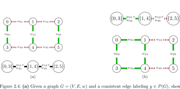
0 1 2 3 4 5 w01 w12 w34 w45 w03 w14 w25 {0,3} w01+ {1,4} {2,5} w34 w12+ w45 (a) {0,3} w01+ {1,4} {2,5} w34 w12+ w45 0 1 2 3 4 5 w01 w12 w34 w45 w03 w14 w25 (b)

Figure 2.4: (a)Given a graphG= (V, E, w)and a consistent edge labelingy∈P(G), shown by solid and dotted lines, the contraction graphGy= (Vy, Ey, wy)is constructed by

contracting uncut edges inGw.r.t.y.(b)Given an edge labelingy¯of a contracted graph Gy = (Vy, Ey, wy), we can back project the edge labeling to the original

graph.

2.4.2 Polyhedral Interpretation

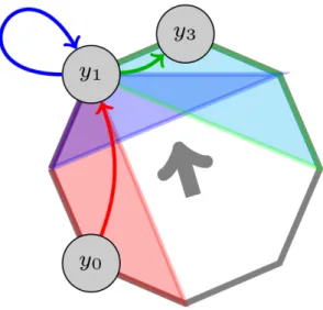
A polyhedral interpretation of fusion moves is shown in Fig.2.6. In each iteration the current and proposed segmentation define an inner polyhedral approximation of the original polytope. This interpretation holds for original fusion moves [96] as well as for the proposed CC-Fusion.

In our case, optimizing over the inner polytope is the same kind of problem as the original multicut polytope, but much smaller. Furthermore, the cost do not change and an improvement in the smaller polytope will be the same in the original graph, as shown in Theorem 1.

The choice of the proposal defines the shape of the inner polytope. In the given toy example, the first (red) polytope gives a huge improvement, the second proposal defines the blue polytope which does not lead to an improvement. The third proposal generates the green polytope that includes the globally optimal solution.

This procedure is fundamentally different from common polyhedral multicut meth-ods [65,67], which tighten an outer relaxation of the multicut polytope and contrary to our method do not operate in the feasible domain.

(27)

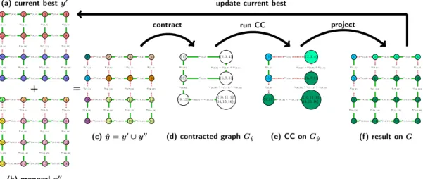
1 2 3 4 5 6 7 8 9 10 11 12 13 14 15 16 w(1,2) w(2,3) w(3,4) w(5,6) w(6,7) w(7,8) w(9,10) w(10,11) w(11,12) w(13,14) w(14,15) w(15,16) w(1,5) w(5,9) w(9,13) w(2,6) w(6,10) w(10,14) w(3,7) w(7,11) w(11,15) w(4,8) w(8,12) w(12,16) + 1 2 3 4 5 6 7 8 9 10 11 12 13 14 15 16 w(1,2) w(2,3) w(3,4) w(5,6) w(6,7) w(7,8) w(9,10) w(10,11) w(11,12) w(13,14) w(14,15) w(15,16) w(1,5) w(5,9) w(9,13) w(2,6) w(6,10) w(10,14) w(3,7) w(7,11) w(11,15) w(4,8) w(8,12) w(12,16) = 1 2 3 4 5 6 7 8 9 10 11 12 13 14 15 16 w(1,2) w(2,3) w(3,4) w(5,6) w(6,7) w(7,8) w(9,10) w(10,11) w(11,12) w(13,14) w(14,15) w(15,16) w(1,5) w(5,9) w(9,13) w(2,6) w(6,10) w(10,14) w(3,7) w(7,11) w(11,15) w(4,8) w(8,12) w(12,16) {1} {2,3,4} {5} {6,7,8} {9,13} {_14,15,10,11,12,₁₆_} w(1,2) w(1,5) w(1,5) w(5,6) w(5,9) w(9,10)+w(13,14) w(2,6)+w(3,7)+w(4,8) w(6,10)+w(7,11)+w(8,12) {1} {2,3,4} {5} {6,7,8} {9,13} {_14,15,1610,11,12,_} w(1,2) w(1,5) w(1,5) w(5,6) w(5,9) w(9,10)+w(13,14) w(2,6)+w(3,7)+w(4,8) w(6,10)+w(7,11)+w(8,12) 1 2 3 4 5 6 7 8 9 10 11 12 13 14 15 16 w(1,2) w(2,3) w(3,4) w(5,6) w(6,7) w(7,8) w(9,10) w(10,11) w(11,12) w(13,14) w(14,15) w(15,16) w(1,5) w(5,9) w(9,13) w(2,6) w(6,10) w(10,14) w(3,7) w(7,11) w(11,15) w(4,8) w(8,12) w(12,16)

contract run CC project

update current best (a) current besty0

(b) proposaly00

(c)yˆ=y0_∪_y00 _{(d) contracted graph}_G

ˆ

y (e) CC onGyˆ (f) result onG

Figure 2.5: To fuse a current best segmentation y0 (2.5a) with a proposal segmentation y00

(2.5b) we propose the following algorithm:yˆis defined as y0+y00as in (2.5c). The

contraction graph (2.5d)Gˆyis constructed by contracting all uncut edges inyˆ. The

actual fusion move is solving eq. (2.2) forGyˆas in (2.5e) and projecting the result

back toGas in (2.5f). The result of the fusion move is guaranteed to be no worse

thany0 ory00. Therefore the current best solution can be updated from the result

of the fusion move. In summary, the correlation clustering fusion move algorithm iteratively fuses the current best solution with different proposals.

(28)

Figure 2.6: Each fusion move can be interpreted as an optimization of an inner polytope. Each inner polytope includes the current vertex. Starting withy0we optimize over

the red polytope and findy1 as optimum. Finally, when optimizing over the blue

polytope we stay iny1 as optimum, when optimizing over the green polytope we

(29)

2.4.3 Proposal Generators

As discussed in [96], proposals should have two properties: high quality and large diversity.

A proposal has a high quality if it has a low energy at least in some regions. For high quality proposals the chance that the inner polytope includes a better solution (vertex) is larger than for those with low quality.

Diversity between the individual proposals increases the chances to span diverse in-ternal polytopes, cover with the intersection of inner polytopes a large part of the original polytope and find more likely the globally optimal solution or escape from local minima.

For correlation clustering fusion we add a third property: size. The size of the

con-tracted graph directly depends on the number of connected components of the inter-section of the proposal solution and the current best solution. In one extreme case, where each node is in a separate connnected component, the fusion move is equivalent to solving the original problem. In the other extreme, where the proposal has a single connected component, the current best solution will not change. Therefore the size of the proposals should be small enough, such that solving eq. 2.5 can be done fast enough, but on the other side large enough to define a large internal polytope and therefore a powerful move. To this end we suggest two proposal generators.

Randomized Hierarchical Clustering (RHC): To generate fast energy aware proposals we can use energy based hierarchical clustering (EHC) as defined in Sec.2.3. EHC follows the energy function, therefore thequality of the proposals is high. To get diversity among the different proposal, we add normally distributed noiseN(0, σehc)to

each edge weight. To get proposals of the desiredsize, we use a different stop condition

for EHC, and stop only if a certain number of connected components is reached. Randomized Watersheds (RWS): Watersheds have become quite popular for graph segmentation and have a strong connection to energy minimization [45]. The edge weighted watershed algorithm [109] with random seeds can be used to find cheap proposals. To improve quality we do not use n seeds distributed uniformly over all

nodes but use the following. We draw n/2 negative edges, and assign different seeds

to the endpoints of each edge. Doing so, a random subset of negative edges is forced to be cut within each proposal. For additional diversity, noise N(0, σws) is added to

(30)

2.5 Experiments

In our experiments we compare to the following methods with publicly available im-plementation. For CGC [29] we used a branch of OpenGM 1 and for KL [76] the implementation in OpenGM2_{. For integer multicuts (}_MC-I_{) and relaxed multicuts}

(MC-R) [65] we modified OpenGM2, as described in Sec.2.5.2.

From the field of data-mining we compare to the PIVOT-algorithm [3] followed by a round of BOEM [55] denoted by PIVOT-BOEM3_{. This implementation uses full}

adjacency matrices it does not scale and cannot be applied to all datasets. We also run classical fusion moves [96] (Fusion) and select distinct labels for the two candi-date segmentations. According to [29], CGC is faster and gives better energies than PlanarCC [146] and Expand & Explore [23]. Therefore we exclude those in our exper-iments.

We compare all of the above to the following methods suggested in the present pa-per: Energy Based Hierarchical Clustering (EHC), as described in Sec. 2.3. CGC warm started with the solution from EHC (EHC-CGC). The proposed correlation cluster fusion algorithm with EHC-based and watershed-based proposals and MC-I and CGC as subproblem solvers (CC-Fusion-HC-MC,-HC-CGC,-WS-MC, and -WS-CGC) respectively. We set the number of connected components in the propos-als to 10% of the number of nodes of and use random edge noise with σ = 1.5. As

stopping condition we choose 104 iterations and 100iterations with no improvement.

All experiments were run on Intel Core i5-4570 CPUs with 3.20 GHz, equipped with 32 GB of RAM. In our evaluation we make no use of multiple threads. The methods were stopped once they exceed 30 minutes at the next possible interrupt point.

2.5.1 Datasets

Social Networks.One important application for large scale correlation clustering are social networks. We consider two of those networks from the Stanford Large Network Dataset Collection4_{. Both networks are given by weighted directed graphs with edge}

weights −1 and +1. The first network is called Epinions. This is a who-trust-whom

online social network of a general consumer review site. Each directed edge a → b

indicates that user a trusts or does not trust user b by a positive or negative

edge-weight, respectively. The network contains131828nodes and841372edges from which

1

github.com/opengm/opengm/tree/cgc-cvpr2014

(31)

85.3% are positively weighted. The second network is called Slashdot. Slashdot is a

technology-related news website known for its specific user community. In 2002 Slash-dot introduced the SlashSlash-dot Zoo feature which allows users to tag each other as friend or foe. The network was obtained in November 2008 and contains 77350 nodes and

516575 edges of which76.73%are positively weighted.

We consider the problem to cluster these graphs such that positively weighted edges (E_→+) link inside and negatively weighted edges (E_→−) between clusters. In other words

friends and people who trust each other should be in the same segment and foes and non-trusting people in different clusters. To compensate the large impact of nodes with high degree we can normalize the edge weights such that each person has the same impact on the overall network, by enforcing.

X

i→j∈E→

|wi→j|= 1 ∀i∈V, degout(i)≥1 (2.7)

We define the following energy function

J(y) = X i→j∈E+→ yij ·wi→j+ X i→j∈E→− (yij −1)·wi→j = X ij∈E yij ·(wi→j +wj→i) | {z } wij +const (2.8)

which is zero if the given partitioning does not violate any relation and larger otherwise. We name these two datasets social nets andnormalized social nets.

Network Modularity Clustering. As another example for network clustering we use the modularity-clustering models from [70] which are small but fully connected.

2D and 3D Image Segmentation To segment images or volumes into a previously unknown number of clusters, correlation clustering has been used [8,9].

Starting from a super-pixel/-voxel segmentation, correlation clustering finds the clus-tering with the lowest energy. The energy is based on a likelihood of merging adja-cent super-voxels. Each edge has a probability to keep adjaadja-cent segments separate (p(yij = 1)) or to merge them (p(yij = 0)). The energy function is

J(y) = X ij∈E yij ·log p(yij = 0) p(yij = 1) +log1−β β | {z } wij (2.9)

(32)

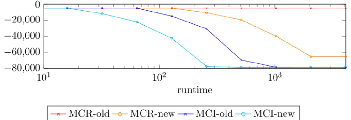
101 102 103 −80,000 −60,000 −40,000 −20,000 0 runtime

MCR-old MCR-new MCI-old MCI-new

Figure 2.7: Comparison of the Multicut implementation of OpenGM and our modified imple-mentation, which improves the runtime. However, for large scale problems it still does not scale.

We use the publicly available benchmark instances from [69,70]. For 2D images from the Berkeley Segmentation Database [107] we took the segmentation problems called

image-seg [8,69]. For 3D volume segmentation we use the models knott-3d-150, -300

and-450 from [9,70] as well as the large instance from the3d-seg model [8,69]. These

instances have underlying cube sizes of 1503, 3003, 4503, and 9003, respectively. We

also requested larger instances from the authors of [9] who kindly provided us the dataset knott-3d-550 with cube size 5503.

2.5.2 Improvements for the Multicut Algorithm

When using the publicly available implementation in OpenGM2_{, we have noticed that}

their implementation has some limitations on large problems. This results in a very slow separation and we make the following modifications. Firstly, we used index-min-heap [122] within the shortest path search by the Dykstra algorithm, which speeds

up MC-R. Secondly, we follow [9] and search for shortest paths and add those only if they are non-chordal,instead of searching for the shortest non-chordal path during the separation procedure. In [9] this was used for MC-I only. For MC-R this search procedure is not sufficient and needs to be followed by a search for shortest non-chordal paths. Fig. 2.7 shows the improvements with our modifications compared to the implementation in OpenGM for the knott-3d-450 dataset. This procedure is one magnitude faster, but might cause a few extra outer iterations.

(33)

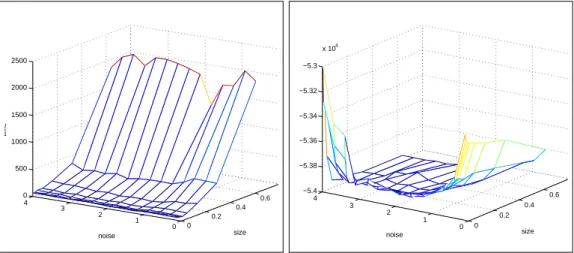
2.5.3 Parameter Choice for CC-Fusion

Beside the choice of the proposal generator and fusion method, CC-Fusion has some more parameters, which need to be set. The most crucial one is the number of segments in the proposal. For HC we also have to set the noise which is used to generate diversity. Fig. 2.8 shows an evaluation of the impact of this parameters for a single instance of knott-3d-450 averaged over several random seeds. The runtime depends on the number of clusters in the proposal (Fig.2.8left), which controls the size of the auxiliary move problems. The level of noise has no major impact on the runtime. The energy of the final solution improves with finer proposals since this increases the search space of the moves. The level of noise has to be large enough to generate diverse proposals, but not too large as this would lead to proposals with low quality. As shown in Fig. 2.8right the useful parameter set is quite large. This allows us to use the same parameters for

all experiments. However we would like to note that in practice we can improve the

performance by adjusting these parameters for the specific problem setting.

0 0.2 0.4 0.6 0.8 0 1 2 3 4 0 500 1000 1500 2000 2500 size noise time 0 0.2 0.4 0.6 0.8 0 1 2 3 4 −5.4 −5.38 −5.36 −5.34 −5.32 −5.3 x 104 size noise value

Figure 2.8: Empirical evaluation of the impact of noise used for proposal generation and the size of the proposals. Proposals with many segments cause longer runtime. Noise seemed not to be a critical parameter but should be selected large enough.

2.5.4 Evaluation

For the evaluation of the different methods on the datasets introduced in Sec. 2.5.1, we show zoomed anytime plots in Fig. 2.9 and variation of information (VOI) [108] and rand index (RI) [116] of the final solutions in Tab. 2.1. Anytime plots with no

(34)

zooming and a detailed evaluation are given in the supplementary material. For social-nets CC-Fusion methods provide the best results for the first minutes . Only CGC

and HC-CGC are able to find better solutions after more than 1000 seconds. MC-I and MC-R cannot be applied to such large problems. We believe that with better proposal generators, which are more suited for such network problems, we can improve CCFusion. One candidate for such a generator would be a scalable implementation of the PIVOT algorithm. For modularity-clustering CC-Fusion performs on par with

competitive methods, even though CC-Fusion and the used parameters have not been designed and chosen for this type of problem. In particular, it does a better job than MC-I. Forimage-segCC-Fusion is faster than other methods and competitive in terms

of energy, VOI, and RI. Because the models are designed to have a high boundary recall (oversegmentation), classical fusion, which returns undersegmentations, has best VOI but worse RI and energy. Proposals generated by EHC are a bit better than WS-based ones. For the knott-datasets CC-Fusion-HC-MC and CC-Fusion-WS-MC have

a better performance with increasing problem size compared to competitive methods,

cf. Fig. 2.9(b-e). Also in terms of VOI and RI they are only slightly worse than the

globally optimal solution found by MC-I. The initialization of CGC by HC, denoted by HC-CGC, also improves the performance compared to native CGC. For the largest 3D volume seg-3d, HC-CGC gives the first useful solution, cf. Fig.2.9(f). However, after

a few minutes CC-Fusion-HC-MC and CC-Fusion-WS-MC give much better results and are also overall best in terms of energy, VOI, and RI. Pure EHC, Fusion and PIVOT-BOEM do not give useful results on any dataset.

2.6 Conclusion

We have presented a fast and scalable approximate solver for correlation clustering, named Correlation Clustering Fusion (CC-Fusion). It is orthogonal to previous re-search,i.e. it can be combined with any correlation clustering solver. The best solution

is iteratively improved by a fusion with proposal solutions. The fusion move itself is formulated as correlation clustering on a smaller graph with fewer edges and nodes and can therefore be solved much faster than the original problem. Our evaluation shows that several CC-Fusion algorithms outperform many existing solvers w.r.t. anytime performance with increasing problem size.

(35)

10−1 100 101 102 103 4,500 5,000 5,500 6,000 runtime

(a) image seg

10−1 100 101 102 −4,000 −2,000 runtime (b) knott-3d-150 10−1 100 101 102 103 −30,000 −20,000 −10,000 0 runtime (c) knott-3d-300 10−1 100 101 102 103 −75,000 −70,000 −65,000 runtime (d) knott-3d-450 100 101 102 103 −1.3·105 −1.2·105 −1.1·105 runtime (e) knott-3d-550 10−1 100 101 102 103 8·105 1·106 1.2·106 runtime (f) seg-3d 10−1 100 101 102 103 60,000 80,000 1·105 1.2·105 runtime (g) social nets 10−1 100 101 102 103 2,000 4,000 6,000 8,000 runtime

(h) normalized social nets

10−1 100 101 102 103

−0.4

−0.2 0

runtime

(i) modularity clustering

PIVOT-BOEM HC HC-CGC CGC KL Fusion

MC-R MC-I CC-Fusion-HC-MC CC-Fusion-HC-CGC CC-Fusion-WS-MC CC-Fusion-WS-CGC

Figure 2.9: Among all proposed solvers, Fusion-HC-MC has the best overall anytime perfor-mance. With increasing problem size (2.9b-2.9e and 2.9f) the runtimes of MC-I, MC-R and CGC increase drastically, while the proposed solvers still scale well. For these instances, the EHC started version of CGC outperforms GCG in terms of runtime and energy.

Overall, energy hierarchical clustering based proposals work better than water-shed based proposals. They converge to similar energies but the clustering based approach is faster on all tested instances. On all instances except for modular-ity clustering, it is better to solve the fusion move to optimalmodular-ity (Fusion-HC-MC) than using approximations (FUSION-HC-GCG). The warm EHC started version of GCG (EHC-CGC) performs better than GCG itself, but both are outperformed by the proposed algorithms w.r.t. anytime performance.

(36)

Table 2.1: Evaluation by Variation of Information (VOI) and Rand Index (RI) for datasets with available ground truth.

VOI image-seg knott-3d-150 knott-3d-300 knott-3d-450 3d-seg

PIVOT-BOEM 4.9633 2.9936 4.4986 – – HC 2.5967 1.5477 2.3513 2.9155 2.8395 HC-CGC 2.5164 0.9052 1.7636 2.2256 1.7603 CGC 2.5247 0.9267 1.8822 2.3104 6.8908 KL 2.6432 2.0648 4.1318 4.9270 7.1057 FUSION 2.1406 2.8787 4.0744 4.6616 6.5366 MC-R 2.5471 0.9178 1.6369 2.8710 6.5058 MC-I 2.5367 0.9063 1.6352 2.0037 4.3319 CC-Fusion-HC-MC 2.5319 0.9629 1.6516 2.0801 1.3347 CC-Fusion-HC-CGC 2.4961 0.9679 1.7673 2.3809 2.1347 CC-Fusion-WS-MC 2.5340 0.9629 1.6742 2.0739 1.3334 CC-Fusion-WS-CGC 2.5192 1.0585 2.1344 2.7487 3.3514

RI image-seg knott-3d-150 knott-3d-300 knott-3d-450 3d-seg

PIVOT-BOEM 0.7438 0.7851 0.8792 – – HC 0.7560 0.8139 0.8084 0.7610 0.9651 HC-CGC 0.7724 0.9226 0.8713 0.8433 0.9861 CGC 0.7590 0.9206 0.8666 0.8341 0.6024 KL 0.6400 0.8085 0.6858 0.6409 0.5849 FUSION 0.5480 0.2849 0.1420 0.0998 0.0345 MC-R 0.7822 0.9232 0.8849 0.6713 0.0432 MC-I 0.7821 0.9236 0.8849 0.8670 0.5461 CC-Fusion-HC-MC 0.7801 0.9042 0.8824 0.8573 0.9906 CC-Fusion-HC-CGC 0.7780 0.9031 0.8763 0.8470 0.9775 CC-Fusion-WS-MC 0.7825 0.9042 0.8802 0.8582 0.8895 CC-Fusion-WS-CGC 0.7750 0.8951 0.8596 0.8394 0.9906

(37)

3 Fusion Moves for Lifted Multicut

Partitioning

Many computer vision problems can be cast as an optimization problem whose feasible solutions are decompositions of a graph. The minimum cost lifted multicut problem is such an optimization problem. Its objective function can penalize or reward all decompositions for which any given pair of nodes are in distinct components. While this property has many potential applications, such applications are hampered by the fact that the problem is NP-hard. We propose a fusion move algorithm for computing feasible solutions, better and more efficiently than existing algorithms. We demonstrate this and applications to image segmentation, obtaining a new state of the art for a problem in biological image analysis.

3.1 Introduction and Related Work

In 2011, Andres et al. [8], Bagon and Galun [23], Kim et al. [80, 81] and Yarkony et al. [146] independently proposed formulating the image segmentation problem [17] as a minimum cost multicut problem [25, 46] on a suitable graph. Given, for every pair of neighboring nodes, a cost or reward (negative cost) to be paid if these nodes are assigned to distinct components, the minimum cost multicut problem consists in finding a decomposition of the graph with minimal sum of costs. In 2015, Keuper et al. [78], using a construction from [7], proposed the minimum cost lifted multicut

problem, a generalization with an identical feasible set whose objective function can assign a cost or reward to every pair of nodes, not just neighboring ones. These

non-local interactions are represented in the graph by “lifted” edges which are subjected to slightly different constraints than the regular edges. The introduction of lifted edges is appealing for image segmentation, because non-local interactions can now be added without losing two key advantages of the multicut: (i) Every feasible solution of the optimization problem corresponds to a decomposition of the graph, i.e. to a consis-tent segmentation. (ii) No assumptions on the number or size of segments are made, making the method applicable in the typical and important scenario where such prior knowledge is not available. Since standard and lifted multicut are both NP-hard

(38)

in-teger linear programming problems [25,46] – even for planar graphs [22,142] – this paper proposes a new family of efficient heuristics inspired by [44,96] and on the basis of fusion moves [66,96] .

So far, the computer vision community has studied three classes of algorithms address-ing optimization problems of this type: (i) branch-and-cut algorithms [8, 9, 72] that converge to an optimal integer solution but do not admit polynomial time complexity bounds and are too slow for lifted multicuts; (ii) linear programming relaxations with subsequent rounding to an integer solution [68, 72, 146] which can yield a log-factor approximation [46] in polynomial time; (iii) constrained search algorithms [12,29,78] that find approximate integer solutions directly in polynomial time. Although no the-oretical guarantees are known for the latter approximations, they tend to be better than relaxation followed by rounding.

Constrained search algorithms for the lifted multicut problem were introduced in [78]. They generalize multicut algorithms of the Kernighan/Lin [76] type from [12] and greedy additive edge contraction from [29]. We show in this chapter that fusion move algorithms for the multicut as proposed in [27] can be generalized as well and actually perform better in terms of approximation quality and speed.

3.1.1 Contribution

With this chapter, we make the following contributions:

1. We generalize the fusion move algorithm [27] into a new constrained search algorithm for the minimum cost lifted multicut problem defined in [78].

2. We show that our algorithm outperforms the constrained search algorithms of [78] on the same problem instances in approximation quality and speed. 3. We introduce novel non-local potentials for the segmentation problem and

in-corporate them into a lifted multicut formulation of the objective.

4. We apply the proposed algorithm to the biological image segmentation bench-mark [21,37], achieving the highest accuracy known at the time of writing.

3.2 Optimization Problem

3.2.1 Minimum Cost Multicut Problem

(39)

solu-necessary basic definitions and otherwise refer to [41,56] for details.

Adecomposition of a graph is a partition of the node set into connected subsets. More

rigorously, a decomposition of a graph G = (V, E) is a partition Π of the node set

V such that, for every U ∈ Π, the subgraph of G induced by U is connected. Every

decomposition of a graph can be identified with the set of edges that straddle distinct components. Such subsets of edges are called the multicuts of the graph.

A subset M ⊆ E of edges is a multicut of G iff there exists a decomposition Π of

G such that M is the set of edges straddling distinct components. Moreover, M is a

multicut of G iff no cycle in the graph intersects with M precisely once. Rigorously,

for every cycle Y ⊆ E of G: |M ∩Y| 6= 1. This characterization is intuitive: If one

transitions from one component to another along the cycle, one needs to transition back before returning to the node from which one has started. It is used to state the minimum cost multicut problem:

For every graph G= (V, E) and every c :E → R, the instance of the minimum cost

multicut problem w.r.t. Gand cis the optimization problem

min x∈{0,1}E X e∈E cexe (3.1) subject to ∀Y ∈cycles(G) ∀e∈Y : xe≤ X e0_∈_Y_\{_e_} xe0 . (3.2)

3.2.2 Minimum Cost Lifted Multicut Problem

The minimum cost multicut problem has a limitation: A multicut makes explicit only for neighboring nodes whether these nodes are in distinct components of the

decom-position induced by the multicut. It does not make this explicit for non-neighboring

nodes. Thus, the cost function can introduce only for pairs of neighboring nodes a cost or reward to be paid by feasibles solutions that assign these nodes to distinct components. It cannot introduce such a cost for pairs of non-neighboring nodes. As illustrated in Fig.3.1, simply considering a graph with more edges does not overcome this limitation in general.

This limitation led Andres [7] to define the minimum cost lifted multicut problem w.r.t. one graphG= (V, E)whose decompositions are identified with feasible solutions,

and a possibly larger graphG0 = (V, E0)withE⊆E0 for whose every edgevw∈E0 it

is made explicit whether the nodes v and ware in distinct components. By assigning

a cost cvw∈Rto this edge, one can penalize or reward precisely those decompositions ofG(!) for which the nodesv andware in distinct components. This property is used

(40)

for image segmentation in [78]. We recall the minimum cost lifted multicut problem from [7, Def. 10].

For any graphs G = (V, E) and G0 = (V, E0) with E ⊆ E0 and every c : E0 → _R, the instance of the minimum cost lifted multicut problem w.r.t. G, G0 and c is the

optimization problem min x∈{0,1}E0 X e∈E0 cexe (3.3) subject to ∀Y ∈cycles(G) ∀e∈Y : xe≤ X e0_∈_Y_\{_e_} xe0 (3.4) ∀vw∈E0\E ∀P ∈vw-paths(G) : xvw≤ X e∈P xe (3.5) ∀vw∈E0\E ∀C∈vw-cuts(G) : 1−xvw ≤ X e∈C (1−xe) . (3.6)

The cycle constraints (3.4) are identical to those in (3.2). Additional constraints (3.5) and (3.6) ensure, for every edge vw ∈ E0\E that xvw = 0 if (3.5) and only if (3.6)

v and w are connected in G by a path of edges labeled 0, i.e., iff v and w are in the

same component of Gdefined by the multicutM :={e∈E|xe= 1}of G. Or in other

words, iff a lifted edge (vw ∈E0\E) is not cut, there must be a path of non-cut edges

in the original graph connecting v and w.

3.3 Optimization Algorithm

3.4 Constrained Search Algorithms

Constrained search is a class of heuristic optimization algorithms. In the computer vision community, they are also commonly referred to as move making algorithms. Examples are α-expansion [86]αβ-swap [86], lazy flipping [10] and fusion [96].

Given a map f :X → R and the optimization problemmin{f(x)|x ∈ X}, the idea of constraint search is this: Instead of optimizing f over the entire feasible set X,

which might be hard, start from an initial feasible solution x0 ∈X, optimize f over

a neighborhood N(x0) ⊆ X to obtain a new feasible solution x1. Iff f(x1) < f(x0),

re-iterate, starting from x1. Note that this algorithm does not require that x1 be

optimal.

(41)

v1 v2 v3 v4 v5 v6 −0.5 −0.5 −1 −1 −1 −1 −1 5 (a) Multicut v1 v2 v3 v4 v5 v6 −0.5 −0.5 −1 −1 −1 −1 −1 5 (b) Lifted Multicut

Figure 3.1: Depicted above in (a) is an instance of the minimum cost multicut problem (3.1)– (3.2). The solution is the multicut consisting of those edges that are depicted as dotted lines. I.e. all edges exceptv1v6are cut. Depicted above in (b) is an instance

of the minimum cost lifted multicut problem (3.3)–(3.6) with one edge in E0\E

depicted in green. Here as well, the solution is the lifted multicut consisting of those edges depicted as dotted lines. Note that, unlike in (a), the lifted edge with cost 5 causes the nodesv1 andv6to be connected in Gby a path of edges labeled

0. Thus, positive costs assigned to lifted edges are called anattraction.

min{f(x0)|x0 ∈ N(x)} is of polynomial time complexity, then every iteration of the algorithm is efficient. If the optimization over the neighborhood is not known to be of polynomial complexity, it can still be less complex or smaller than the original problem and can thus be tractable in practice.

3.4.1 Fusion Move Algorithms

Fusion move algorithms [96] are a class of constrained search algorithms. They consist of two procedures. First is proposal generation that computes, for every feasible

solu-tion x ∈ X given as input, another feasible solution pg(x) ∈ X as output, possibly

in a randomized fashion. Second isfusion, an optimization algorithm that computes a

feasible solution of an optimization problem min{f(x)|x∈N(x)}for a neighborhood

N(x) defined w.r.t. x and pg(x) such that x ∈N(x) and pg(x) ∈N(x), to obtain a

feasible solution x0 with f(x0) ≤ f(x) and f(x0) ≤ f(pg(x)). In a fusion move

algo-rithm, proposal generation and fusion can be combined in different ways, as depicted in Fig. 3.2.

3.4.2 Fusion Moves for the Lifted Multicut Problem

Lempitsky introduced fusion moves for unconstrained quadratic programming in [96]. In chapter 2 we define a fusion move algorithm for the minimum cost multicut prob-lem. Here, we generalize the idea from chapter 2 to the minimum cost lifted multicut

(42)

x x0

FM PG

(a) Serial fusion moves

PG x1 x2 x3 x4 x FM FM FM FM x5 x6 x7 x8 FM FM x9 x10 FM

(b) Parallel fusion moves

Figure 3.2: In a fusion move algorithm, proposal generation (PG) and fusion moves (FM) can be combined in different ways. We implement and study serial fusion moves (a) and parallel fusion moves (b).

problem. The fusion moves are defined in this section. Proposal generators are defined in the next section.

Given any feasible solutions x1 and x2 of the minimum cost lifted multicut problem

(3.3)–(3.6), a constrained minimum cost lifted multicut problem in the variables x ∈ {0,1}E0 _{is defined by (}_3.3_)–(_3.6_{) and the additional constraints}

∀e∈E : xe ≤x1e+x2e . (3.7)

That is, all edges which are labeled 0 (join) in the feasible solutionx1 _and _{the feasible}

solutionx2 are constrained to be labeled 0 in the problem (3.3)–(3.7). By construction, x1 and x2 are feasible solutions of the constrained problem (3.3)–(3.7).

Next, we reduce the constrained minimum cost lifted multicut problem (3.3)–(3.7)

to an unconstrained minimum cost lifted multicut problem w.r.t. a smaller graph

(Lemma 1). The latter problem can be solved by existing algorithms. In practice, we solve it approximatively by means of the Kernighan-Lin-type algorithm published by Keuper et al. [78]. The construction of the smaller graph is depicted in Fig.3.3and is described below.

Let G = (V,E) be the graph obtained from the graph G by contracting the edges

{e∈E|x1_e = 0∧x2_e = 0}1_{. Moreover, let}_E0_⊆ V

2

such that V0W0 ∈ E0 iff there exist

(43)

1 2 3 4

5 6 7 8

9 10 11 12

13 14 15 16

(a) GraphGandE0

{1,2} {3} {4} {5,6,7,9,10}

{8,11,12} {13,14,15,16}

(b) GraphGandE0

Figure 3.3: To perform a fusion move, we solve a minimum cost lifted multicut problem with some edge labels fixed to 0 (join). In (a) such edges are depicted by bold lines. To solve this constrained problem, we reduce it to an unconstrained minimum cost lifted problem w.r.t. a contracted graph, depicted for this example in (b).

V0W0∈ E0:

CV0_W0 = X

{vw∈E0_|_v_∈_V0_∧_w_∈_W0_}

cvw (3.8)

Lemma 1. For every feasible solution X:E0 _{→ {}₀_,₁_}_{of the instance of the minimum} cost lifted multicut problem w.r.t. G,G0 := (V,E0)and C, thex:E0 → {0,1}such that

∀vw ∈E0 : xe=    XV0_W0 if∃V0W0 ∈ E0:v∈V0∧w∈W0 0 otherwise (3.9)

is well-defined and a feasible solution of the constrained minimum cost lifted multicut problem (3.3)–(3.7). Moreover, X vw∈E0 cvwxvw= X V0_W0_∈E0 CV0_W0X_V0_W0 . (3.10)

Proof. If there exist V0W0 ∈ E0 such that v ∈ V0 and w ∈ W0, then V0 and W0 are

unique (becauseV is a partition of V). Thus, x is well-defined.

The feasible solution X defines a decomposition of G (because M := {V0W0 ∈ E |XV0_W0 = 1} is a multicut of G). Every decomposition of G induces a

decompo-sition of G (as the node set V of G is itself a decomposition of G). The multicut

by edgese∈Efor whichx1e= 0andx2e= 0. In addition, for everyV0W0∈

V 2

, we haveV0W0∈ E iff there existv∈V0 andw∈W0such thatvw∈E.

(44)

M :={vw∈E|xvw= 1} of this decomposition ofGis defined by the multicut Mof

G by (3.9) (by definition ofG). Thus,x satisfies (3.4).

Moreover, for every vw ∈E0\E, we have xvw = 0 iff v is connected to w by a path

P inG withxP = 0 (by (3.9) and definition of G and E0). Thus, x satisfies (3.5) and

(3.6). Finally, (3.10) holds by (3.8) and (3.9). 3.4.3 Proposal Generation for the Lifted Multicut Problem

As pointed out in [96], a proposal generator is designed with four objectives in mind. Firstly, proposed feasible solutions should be diverse. Otherwise, the fusion move

al-gorithms can get trapped in local minima. Secondly, some proposed feasible solutions should be good. Otherwise, the fusion move algorithms cannot get close to the

opti-mum. In the context of the minimum cost lifted multicut problem, a feasible solution is good if the recall of edges that are cut in an optimal solution is close to 1. Thirdly, the proposed feasible solutions should be sparse. In the context of the minimum cost

lifted multicut problem, a feasible solutions is sparse if the precision of edges that are cut in an optimal solution is close to 1. Fourthly, the proposed feasible solutions should be cheap, i.e., proposals should be computable efficiently and in parallel. We

study three proposal generators that emphasize different design objectives.

Randomly Perturbed Proposals. In order to obtain a proposal of high quality efficiently, we apply greedy additive edge contraction (GAEC) [78]. The key idea of this algorithm is to greedily contract edges with maximum cost until this maximum cost is equal to or smaller than zero. In order to get diverse solutions, we follow [27] and add normally distributed noise of zero mean to edge costs. In order to control the sparsity of the proposal, we replace the stopping criterion of GAEC and continue until a maximum allowed number of components is reached.

Subgraph Proposals. In order to obtain an objective-aware proposal for a large problem instance, we solve the minimum cost lifted multicut problem for a small subgraph. Technically, the procedure works as follows: We choose a center nodev∈V

and the subgraph induced by the setU of all nodes within a fixed path-length distance

from v. For E0 := {vw ∈E|v /∈ U ∧w /∈ U} and E1 := {vw ∈E|v ∈ U ∧w /∈ U},

we solve the instance of the minimum cost lifted multicut problem w.r.t. the graph G

and the cost function c, with the additional constraints

∀e∈E0 : xe= 0 (3.11)

∀e∈E1 : xe= 1 . (3.12)