Machine Learning Methods for
Autonomous Object Recognition and
Restoration in Images
By:
Ruilong Chen
A thesis submitted in partial fulfilment of the requirements for the degree of
Doctor of Philosophy
Department of Automatic Control and Systems Engineering University of Sheffield
Abstract
Image recognition and image restoration are important tasks in the field of image pro-cessing. Image recognition are becoming very popular due to the state-of-the-art deep learning methods. However, these models usually require big datasets and high com-putational costs, which could be challenging. This thesis proposes an online learning framework that deals with both small and big datasets. For small datasets, a Cauchy prior logistic regression classifier is proposed to provide a quick convergence, and the online weight updating scheme is efficient due to the previously trained weights be-ing reused. For big datasets, convolutional neural network could be implemented. For image recognition, non-parametric classifiers are often used for image recogni-tion such as K-nearest neighbours, however, K-nearest neighbours are vulnerable to noise and high dimensional features. This thesis proposes a non-parametric classi-fier based on Bayesian compressive sensing; the developed classiclassi-fier is robust and it does not need a training stage. For image restoration, which is usually performed before image recognition as a preprocessing process. This thesis proposes such a joint framework that performs image recognition and restoration simultaneously. In image restoration, image rotation and occlusion are common problems but convo-lutional neural networks are not suitable to solve these due to the limitation of the convolutional process and pooling process. This thesis develops a joint framework based on capsule networks. The developed joint capsule framework could achieve a good result on recognition, image de-noising, recovering rotation and removing occlusion. The developed algorithms have been evaluated for vehicle logo
restora-tion and recognirestora-tion, however, they are transferable to other implementarestora-tions. This thesis also developed an automatic detection and recognition framework for badger monitoring for the first time. Badger plays a key role in the transmission of bovine tuberculosis, which is described by government as the most pressing animal health problem in the UK. An automatic badger monitoring system could help researcher to understand the transmission mechanisms and thereby to develop methods to deal with the transmission between species.
Acknowledgements
First and foremost, I would like to thank my supervisor Prof. Lyudmila Mihaylova for her continuous support. It has been my honour to be one of her PhD students. She encouraged me though my whole PhD study with great enthusiasm and patience. I appreciate her encouragement and support for guiding my PhD. Also, I will never forget that she helped me amend papers sentence by sentence. She helped me to build social connections with other universities and companies, which is very helpful. I could not have imagined having a better supervisor for my PhD study.
I would like to express my gratitude to my second supervisor Dr. Wei Liu, for the insightful discussions. I would also like to thank Dr. Matthew Hawes, for his continuous help and valuable suggestions in writing academic papers. During the PhD study, I have also appreciated the knowledge sharing from collaborations with Dr. Olga Isupova, Dr. Jingjing Xiao, Dr. Hao Zhu and Dr. Ruth Little.
I would like to thank my wife, Sofiana Millati, for her valuable care and love. I am so lucky to have her and she makes my PhD life very happy. I would also like to thank my best friend in Sheffield, Bo Zhang, for his tremendous support and valuable advice. I am grateful to my parents and my sister, for always providing me with unconditional support in my life.
Contents
Abstract iii
Acknowledgements v
List of Symbols and Notations xii
Nomenclature xiv
List of Figures xviii
List of Tables xx 1 Introduction 1 1.1 Thesis Outline . . . 2 1.2 Key Contributions . . . 4 1.3 Publications . . . 5 2 Literature Review 7 2.1 Traditional Methods for Image Recognition . . . 7
2.1.1 Image Features . . . 8
2.1.2 Classification . . . 15
2.2 Deep Learning Framework for Image Recognition . . . 20
2.3 Online Learning for Vehicle Logo Recognition . . . 23
2.4 Back-propagation Bayesian Compressive Sensing Classifier . . . 25
Contents
2.6 Summary . . . 29
3 Online Learning for Vehicle Logo Recognition 31 3.1 Introduction . . . 31
3.2 Cauchy Prior Logistic Regression . . . 33
3.3 Conjugate Gradient Descent . . . 38
3.4 Online Weight Updating . . . 39
3.5 Convolutional Neural Networks for Online Learning . . . 41
3.6 Performance Evaluation . . . 43
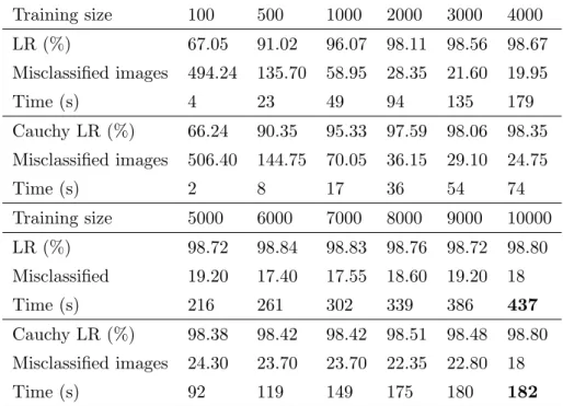
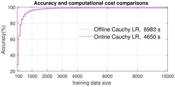
3.6.1 Logistic Regression with the Cauchy Prior Logistic Regression 45 3.6.2 Online and Offline Cauchy Prior Logistic Regression . . . 46
3.6.3 Convolutional Neural Networks for Large Dataset . . . 48
3.7 Summary . . . 51
4 Spatial Invariant Feature Transform and Back-propagation Bayesian Compressive Sensing Classifier 53 4.1 Introduction . . . 53
4.2 Spatial Scale Invariant Feature Transform . . . 54
4.3 Back-propagation Bayesian Compressive Sensing . . . 57
4.3.1 Bayesian Compressive Sensing . . . 57
4.3.2 Back-propagation Bayesian Compressive Sensing with the Column-based Subspace Sampling . . . 62
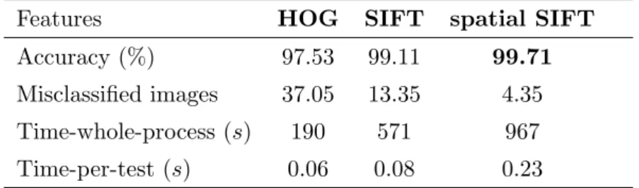
4.4 Performance Evaluations on Spatial Scale Invariant Feature Transform 65 4.4.1 Feature Comparisons . . . 65
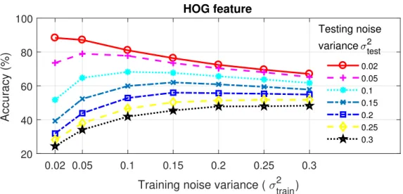
4.4.2 Feature Robustness to Noise . . . 68
4.5 Performance Evaluations on Non-parametric Classification Methods . 71 4.5.1 Evaluations on the Vehicle Logo Recognition Dataset . . . 71
4.5.2 Performance Evaluation for Scene Recognition . . . 79
Contents
4.6 Summary . . . 83
5 Learning Capsules and Joint Frameworks 85 5.1 Introduction . . . 85
5.2 Joint Framework for Recognition and Restoration by Convolutional Neural Networks . . . 86
5.3 Learning Capsules for Recognition and Restoration . . . 89
5.4 Performance Evaluation . . . 94
5.4.1 Capsule Networks for Classification . . . 95
5.4.2 Joint Framework for Image Recognition and Restoration . . . 98
5.5 Summary . . . 106
6 Wildlife Monitoring Based on Deep Learning Methods 107 6.1 Introduction . . . 108
6.2 Deep Learning for Badger Recognition . . . 109
6.2.1 Badger Recognition Framework 1 . . . 110
6.2.2 Badger Recognition Framework 2 . . . 111
6.3 Detection Algorithm in Videos . . . 112
6.4 Performance Evaluation on the Badger Dataset . . . 115
6.4.1 Dataset Generation . . . 115
6.4.2 Badger and Non-Badger Classification . . . 116
6.4.3 Multinomial Classification Based on the Badger Dataset . . . 119
6.4.4 Detection and Classification to Videos . . . 121
6.5 Summary . . . 122
7 Conclusions and Future Works 123 7.1 Conclusions . . . 123
Contents
A Back-propagation Compressive Sensing Extended and the Deep
Learn-ing Architecture in an External Dataset 127
A.1 Marginal Likelihood Maximisation . . . 127 A.2 Evidence Approximation . . . 130 A.3 Deep Learning Framework Parameters on the External Dataset . . . 132
B Deep Learning Framework Parameters for Badger Recognition 133
List of Symbols and Notations
A list of the symbols and notations used in this thesis is defined below. The defini-tions will be used throughout unless otherwise stated.
x Vector X Matrix x∗ A testing data ˆ x The estimation of x xT, XT Transpose of x, X min Minimum max Maximum
arg min Argument that minimises
arg max Argument that maximises
PN
i=1 Sum operation from index 1 to N QN
i=1 Production operation from index 1 to N
df(x)
dx First derivative of the functionf(x) with respect to a variable x
∂f(x,y)
∂x Partial derivative of the function f(x, y) with respect to a
Contents
N(µ,Σ) Normal distribution with mean µand covariance Σ p(·) Probability operator
p(·|·) Conditional probability operator
RM Real numbers of dimensions M
∝ Proportional to
ln(·) The natural logarithm
exp(·) Exponential function
|| · ||1 l1-norm
|| · ||2 l2-norm
|| · ||F Frobenius norm
∗ The convolutional operation
s.t. Subject to
| · | The determinant
Nomenclature
BBCS Back-propagation Bayesian Compressive Sensing
BCS Bayesian Compressive Sensing
BOW Bag of Words
bTB Bovine Tuberculosis
CNNs Convolutional Neural Networks
CS Compressive Sensing
DoG Difference of Gaussian
HOG Histogram of Oriented Gradient
ITS Intelligent Transportation Systems
KNN K Nearest Neighbours
LR Logistic Regression
PCA Principle Component Analysis
PSNR Peak Signal-to-Noise Ratio
ReLU Rectified Linear Unit
Contents
SGD Stochastic Gradient Descent
SIFT Scale Invariant Feature Transform
SURF Speeded Up Robust Features
SVM Support Vector Machine
List of Figures
2.1 The ways in which humans and computers understand an image . . . 8 2.2 The process of dividing an image into cells and blocks in the histogram
of gradient algorithm . . . 10 2.3 An example of scale invariant feature transform descriptors . . . 13 2.4 An example of data can be separated by infinite lines . . . 16 2.5 An example of the maximum margin in the support vector machines . 17 2.6 A typical convolutional neural network architecture example . . . 21 2.7 A typical restoration architecture based on convolutional neural
net-works . . . 28
3.1 The developed vehicle logo recognition framework for increasing size of dataset . . . 31 3.2 The developed online recognition framework for vehicle logo recognition 40 3.3 The developed convolutional neural network architecture . . . 42 3.4 Image examples of the vehicle logo dataset . . . 43 3.5 Examples of some challenge images in the testing dataset . . . 44 3.6 Accuracy and computational costs comparisons between logistic
re-gression and Cauchy prior logistic rere-gression when the dataset size is increasing . . . 46 3.7 Offline and online Cauchy prior logistic regression comparisons up to
List of Figures
3.8 Accuracy and computational costs comparisons between offline and online Cauchy prior LR up to 3000 random training images . . . 48 3.9 An example of three testing images and the effects by adding Gaussian
white noise with different noise variances . . . 50
4.1 Illustration of spatial pyramid interest points. . . 55 4.2 Illustration of the bag of words representation model . . . 56 4.3 The developed recognition framework by using spatial scale invariant
feature transform . . . 57 4.4 An example of a training image and its effects by adding Gaussian
noises . . . 68 4.5 Accuracy of the recognition framework by using the histogram of
gra-dient . . . 69 4.6 Accuracy of the recognition framework by using the scale invariant
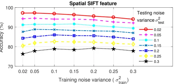
feature transform . . . 70 4.7 Accuracy of the recognition framework using the spatial scale invariant
feature transform . . . 70 4.8 Illustration of some challenging images . . . 73 4.9 Noise robustness comparisons of KNN, SRC and SBCS using the full
training dataset . . . 74 4.10 The total number of local features detected from images with different
noise variances . . . 75 4.11 Noise robustness comparisons ofKNN, SRC and SBCS when there are
10% training examples in each class using the column-based subspace sampling. . . 77 4.12 Noise robustness comparisons ofKNN, SRC and SBCS when there are
1% training examples in each class using the column-based subspace sampling . . . 78 4.13 Image examples in the traffic scene dataset . . . 80
List of Figures
4.14 An example of a traffic scene image with Gaussian noises . . . 81 4.15 An example of an image from external dataset with Gaussian noises . 82
5.1 A general joint framework for image restoration and recognition . . . 86 5.2 The joint convolutional neural network framework for image
recogni-tion and restorarecogni-tion . . . 89 5.3 The architecture of capsule networks for classification . . . 92 5.4 The capsule generation process in the proposed primary capsule layer 92 5.5 The reconstruction process of the capsule networks . . . 93 5.6 The accuracy of the convolutional neural networks and the developed
capsule networks on the original testing data . . . 95 5.7 Ilustration of rotation and noise effects on 20 random testing images . 96 5.8 The accuracy of the convolutional neural networks and the developed
capsule networks on the challenge testing dataset . . . 97 5.9 Twenty testing images for illustration purpose . . . 98 5.10 De-noising results by the joint convolutional neural networks and the
joint capsule networks . . . 99 5.11 Rotation restoration result by the joint convolutional neural networks 101 5.12 Rotation restoration result by the joint capsule networks . . . 102 5.13 Occlusion restoration results by the joint convolutional neural
net-works and the joint capsule netnet-works . . . 103 5.14 The restoration results of the joint convolutional neural networks and
joint capsule networks with Gaussian noise, rotation and concussion . 105
6.1 The architecture of badger recognition framework 1 . . . 110 6.2 The architecture of badger recognition framework 2 . . . 111 6.3 The diagram of applying the trained convolutional neural networks to
videos . . . 112 6.4 Some random testing images from the badger dataset. . . 116 6.5 Illustration of a detected frame activated by a badger . . . 121
List of Tables
3.1 Performance comparisons between logistic regression and Cauchy prior
logistic regression when dataset size is increasing . . . 45
3.2 Accuracy comparisons between Cauchy prior logistic regression and convolutional neural networks when dataset size is increasing . . . 49
3.3 Comparisons between Cauchy prior logistic regression with convolu-tional neural networks when training and testing images are noisy . . 50
4.1 Performance of histogram of gradient by using different classifiers . . 65
4.2 Classification accuracies by using scale invariant feature transform, according to different dictionary sizes in the k-means clustering . . . 66
4.3 Classification accuracies by using spatial scale invariant feature trans-form, according to different dictionary sizes in thek-means clustering 67 4.4 Computational costs using different features with the logistic regres-sion classifier . . . 68
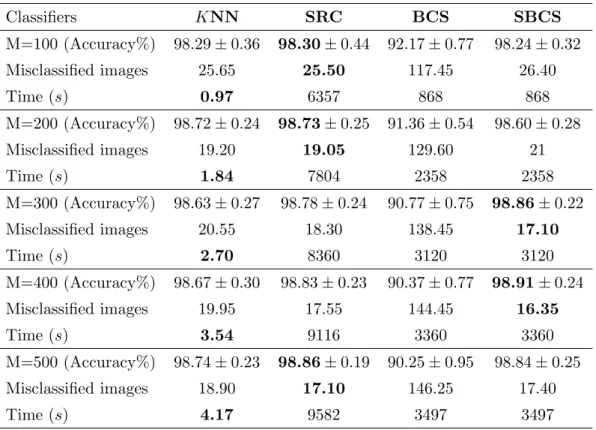
4.5 Non-parametric classifier comparisons . . . 72
4.6 Accuracies obtained using challenging data . . . 73
4.7 Comparisons between using the full and partial dictionaries . . . 76
4.8 Classifier comparisons on traffic scene dataset using features extracted by AlexNet . . . 81
4.9 Classifier comparisons on external dataset using features extracted by AlexNet . . . 82
List of Tables
5.1 Performance of the joint convolutional neural networks and the joint capsule networks on noisy images . . . 100 5.2 Performance of the joint convolutional neural networks on rotated
images . . . 101 5.3 Performance of the joint capsule networks on rotated images . . . 102 5.4 Performance of the joint convolutional neural networks and the joint
capsule networks on occluded images . . . 104 5.5 Performance of the joint convolutional neural networks and the joint
capsule networks on combined degradations . . . 105
6.1 Categories and number of images in the badger dataset . . . 115 6.2 Badgers and non-badgers in the badger dataset . . . 117 6.3 The performance of the badger recognition framework 1 without a
re-sampling process . . . 117 6.4 The performance of the badger recognition framework 1 with a
re-sampling process . . . 118 6.5 The performance of the badger recognition framework 2 . . . 118 6.6 The performance of the badger recognition framework 1 without a
re-sampling process . . . 119 6.7 The performance of the badger recognition framework 1 with a
re-sampling process . . . 120 6.8 Result of the badger recognition framework 2 without a re-sampling
process . . . 120 6.9 The performance of the badger recognition framework 2 with a
Chapter 1
Introduction
Image recognition became very popular in many applications following the success of the Convolutional Network Networks (CNNs [1]) in 2012. Before the CNNs, major-ity image recognition frameworks included a hand-crafted feature detection process and a feature description process [1, 2]. Image features transfer an image from the pixel level to a feature level and then features are used for classification purpose. Unlike the traditional hand-crafted feature methods, CNNs automatically learn the image feature by multiple convolutional operations. A CNN framework has many parameters, therefore, big datasets are required in order to learn these parameters. However, big datasets are not always available and the image data are obtained in-crementally in some applications. This leaves the question of what the best solution is for a small dataset or an incremental dataset. In addition, CNNs have recently achieved good results on image restoration such as image de-noising and image super-resolution. However, automatically recovering rotated images and occluded images are challenging tasks but not well studied [3]. Rotation and occlusion are common image degradations and it would be valuable if a degraded image can be recovered to a clear version. Moreover, most existing deep learning frameworks are focusing on dealing with one particular problem such as image recognition and image restora-tion [4]. This appraises the quesrestora-tion of whether we can develop a joint framework that could perform image recognition and restoration simultaneously using a shared
1.1. Thesis Outline
network.
The focus of this thesis is on the development of novel machine learning methods for autonomous image recognition and restoration. Chapter 3 proposes an online recognition framework in order to deal with incremental datasets. Chapter 4 focuses on the development of a spatial image feature method and a non-parametric clas-sification method. Chapter 5 proposes joint frameworks for image recognition and restoration based on CNNs and capsule networks. Chapter 6 develops automatic detection and recognition methods for badger recognition. This thesis starts with the application of Vehicle Logo Recognition (VLR) and some other datasets have been applied. The developed methods could also be extended to other fields.
1.1
Thesis Outline
The structure of the thesis is outlined below:
Chapter 1
introduces the research topic and purpose of this thesis, followed by the outline of this thesis and key contributions in each chapter. Relevant publications are listed in the last section of this chapter.Chapter 2
reviews some fundamental feature methods and classification meth-ods. The state-of-the-art deep learning methods are introduced for image recognition, followed by an overview of methods for VLR and and image restoration.Chapter 3
focuses on online learning, considering a small training image dataset at the beginning. In this case, CNNs would not be appropriate due to the high computational costs and a limited size of training data. A dynamic online learning framework is developed for streaming data where models are updated from small to big datasets. The developed framework includes the Histogram of Oriented Gradient (HOG) feature method and the Cauchy prior Logistic Regression (LR) with the conjugate gradient descent. The Cauchy prior assumes most of the weights are near zero-valued; this results in accurate and quick convergence in the weight up-date scheme. The Cauchy prior LR could be applied online using a weight upup-date1.1. Thesis Outline
scheme, this further decreases the computational costs. When the training data is big enough, the CNNs could be applied in order to further increase the accuracy and the robustness to image degradations such as noise.
Chapter 4
begins with a recognition framework based on the spatial Scale Invariant Feature Transform (SIFT) features. This feature method takes the ad-vantage of considering spatial information of the SIFT features in an image. The spatial SIFT features could increase the robustness to noise by incorporating the geographical information of the local features. This chapter also investigates non-parametric classifiers and proposes a Similarity-based Bayesian Compressive Sensing (SBCS) classifier. The proposed SBCS classifier takes the advantage of the Bayesian approach when compared with the traditional compressive sensing approaches. In addition, a column-based subspace sampling is introduced in order to select rep-resentative samples in the training dataset, aiming at decrease the computational costs while keeping high accuracy. The SBCS proved to be robust to noise, when compared with the state-of-the-art CNNs.Chapter 5
introduces the learning capsules and develops capsule networks for VLR. Capsule networks contain multiple layers similarly as in CNNs, however, the connections between adjacent layers are changed to vector-vector, rather than scalar-scalar in CNNs and in neural networks. This chapter also proposes joint frameworks targeted at simultaneously performing image recognition and restoration tasks. Combining the recognition and restoration could help the weight updating process by a shared network. Image rotation and occlusion are considered in the restoration process. These image degradations can be recovered while giving high recognition accuracies at the same time.Chapter 6
develops an automatic recognition framework for badger moni-toring. Automatic badger monitoring is beneficial to enhance understanding of the transmission of Bovine Tuberculosis (bTB), which is described by government as the most pressing animal health problem in the UK. This is due to thetransmis-1.2. Key Contributions
sions of the disease including cattle-badger, badger-badger and badger-cattle. In this chapter, an image dataset has been created. Based on the created dataset, two recognition frameworks have been developed based on CNNs. The trained recogni-tion frameworks are combined with a video frame detecrecogni-tion algorithm, which aims at selecting frames of interest in videos.
Chapter 7
gives a summary of the thesis and discusses the future work.1.2
Key Contributions
Key contributions of this thesis are highlighted below.
• For the first time, an online recognition framework is developed for VLR; this framework considers both small dataset and big dataset.
• The Cauchy prior LR classifier is proposed with the conjugate gradient de-scent. The developed maximum a posterior model gives a quicker solution when compared with the maximum likelihood model in LR.
• A novel VLR framework has been developed with a spatial SIFT feature method. This framework considers the spatial correlation of different SIFT features and improves the robustness to noise.
• A novel Similarity-based BCS non-parametric classifier is proposed. The Bayesian compressive sensing is applied to estimate the weights vector. The proposed classifier proved to be quicker when compared with the state-of-the-art sparse representation classifier while giving similar recognition results.
• A column-based subspace sampling is developed to pick up representative data from the dataset for VLR. This process significantly decreases the computa-tional costs while keeping the feature space unchanged.
• For the first time, a learning capsule framework is proposed and developed in the field of intelligent transportation systems. The proposed framework
1.3. Publications
achieves higher accuracy and better robustness to image degradations than the state-of-the-art CNNs.
• Joint frameworks are proposed for image recognition and image restoration based on CNNs and capsule networks. The proposed joint framework based on capsules achieves good results on recognition, image de-noising, rotation correction and occlusion removal.
• For the first time, an image dataset is created for badger recognition.
• For the first time, an automatic recognition framework is developed for badger recognition.
• An automatic detection scheme is developed aiming at identifying frames of interest in videos.
1.3
Publications
The author’s publications with relevance to this thesis are listed below:
Peer Reviewed Conference Proceedings
• [P1] R. Chen, M. Hawes, L. Mihaylova, J. Xiao, and W. Liu, “Vehicle logo recognition by using spatial-SIFT combined with logistic regression”, in Proc.
of International Conf. on Information Fusion, Heidelberg, Germany, July
2016, pp.1228-1235
• [P2] R. Chen, M. Hawes, O. Isupova, L. Mihaylova, and H. Zhu, “Online vehicle logo recognition using Cauchy prior logistic regression”, in Proc. of International Conf. on Information Fusion, Xi’an, China, July 2017, pp.1-8
• [P3] R. Chen, M. A. Jalal, L. Mihaylova, and R. Moore, “Learning capsules for vehicle logo recognition”, in Proc. of International Conf. on Information
1.3. Publications
Fusion, Cambridge, UK, July 2018
• [P4] M. A. Jalal, R. Chen, R. Moore, and L. Mihaylova, “American sign lan-guage posture understanding with deep neural networks”, inProc. of Interna-tional Conf. on Information Fusion, Cambridge, UK, July 2018
Journal Publication Under Review
• [P5] R. Chen, M. Hawes, and L. Mihaylova, “Vehicle logo and scene recognition based on back-propagation Bayesian compressive sensing”, Signal Processing, 2018
Journal Publication in Preparation
• [P6] R. Chen, L. Mihaylova, R. Little, R. Cox and R. Delahay “Wildlife mon-itoring with deep learning methods”, Methods in Ecology and Evolution, 2018
Chapter 2
Literature Review
2.1
Traditional Methods for Image Recognition
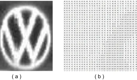
Recognising content in an image is easy for humans as we have advanced visual systems which are good at detecting edges and describing the abstract contents. In contrast, computers are good at describing digitised information such as how many pixels are in an image and what their intensity values are. However, it is challenging for computers to describe the abstract content inside an image. For instance, Figure 2.1 shows how humans and computers see an image. We humans automatically detect a big cycle inside the picture, the ‘V’, and ‘W’ shape inside the cycle as shown in Figure 2.1 (a). We can even understand that the main content is a vehicle logo representing the Volkswagen company if we have the knowledge in advance. In contrast, Figure 2.1 (b) shows how the image is stored in a computer, only intensity values of pixels are recorded. The digital image can be easily influenced by noise, shift, rotations, and occlusions. For example, if one row in the image matrix is deleted, humans find it hard to detect the difference, whereas the matrix stored in the computer has been totally changed.
Even though recognising images is easy for human beings, we still wish to let computers do such tasks as it can save cost and avoid mistakes by human fatigue. One simple way of letting computers recognise a vehicle logo image is to send pixel
2.1. Traditional Methods for Image Recognition
Figure 2.1: The ways in which humans and computers understand an image, respectively.
intensity values from well-segmented logo images directly into a classifier. However, this is not feasible for images of large size due to the computational costs. More importantly, the accuracy is low. For instance, simply reshaping the raw pixel in-tensities into a SVM could only achieve an accuracy of 16.40 % on a vehicle logo dataset (methods developed in chapter 5 could achieve up to 100% accuracy on the same dataset by using the capsule networks). While the dataset has ten classes and a random guess has an expectation of 10 % accuracy according to the probability theory. Hence, more advanced techniques are required for image recognition.
2.1.1
Image Features
In order to let computers recognise the content in an image, hand-crafted features that explore the image pattens are often applied instead of using the raw pixel values. Hand-crafted features define an image by engineering rules. For example, colour information including colour histogram and colour moment is used as image features [5]; Yang et al. [6] use shape and contour information as the image fea-tures; distinguishable edges and corners information is extracted as features in [2, 7]. Presently, automatic feature extraction methods inspired by neurons in the human visual systems have become the mainstream in the field of image recognition. The
2.1. Traditional Methods for Image Recognition
automatic learned features proved to be more accurate when associated with big data [1]. The following introduce different image feature methods, from the tradi-tional hand-crafted features to the state-of-the-art deep learning features.
Global Features
Hand-crafted features can be separated as global features and local features. Global features take all pixels into consideration and represent an image with a single vector. In the following, the well-known global feature method HOG is introduced in detail. HOG was originally introduced as a representation method for human detection [7, 8]. HOG calculates the horizontal gradient Gx and the vertical gradient Gy on
every pixel by use of a 1-D filter [-1, 0, 1]:
Gx(i,j) =I(i+ 1, j)− I(i−1, j), (2.1) Gy(i,j) =I(i, j + 1)− I(i, j−1), (2.2) where I(i, j) is the intensity value at pixel location index (i, j).
Then the horizontal gradient and vertical gradient can be applied to calculate the orientation of gradient θ(i, j) and the magnitude of gradient H(i, j) for every pixel in the image:
θ(i, j) =arctan(Gy(i,j)/Gx(i,j)), (2.3) H(i, j) =qG2
x(i,j)+G 2
y(i,j), (2.4)
whereθ(i, j) andH(i, j) represent the orientation and the magnitude of the gradient at pixel location index (i, j) respectively.
The next step is quantizing the orientation into bins evenly spaced over 0◦−180◦ in order to build an orientation histogram. The image is divided into cells, with a certain number of cells building up a block. Figure 2.2 shows how an image is
2.1. Traditional Methods for Image Recognition
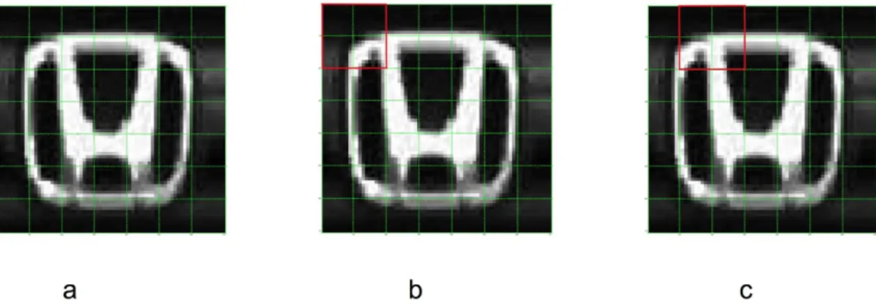
Figure 2.2: The process of dividing an image into cells and blocks in the HOG algorithm. In (a), images are divided into cells, a group of cells form a block denoted as red lines in (b), the block shifts from left to right in (c).
divided into cells and blocks. The original image can be divided into different cells of the same size (Figure 2.2.a). Each cell can be represented as a histogram, with the quantized orientations as histogram bins and the magnitude as weights. Histograms in a block (a block is a 2×2 cell in the example) are concatenated together and get normalised in order to be robust to illuminance variations. The block is then shifted one cell (or one block) forward from either left to right or top to bottom. In the example shown in Figure 2.2, a block is shifted cell by cell; this results in overlaps among adjacent blocks. In the Figure 2.2.b and Figure 2.2.c, the area within red lines indicates the first and second block, respectively. The block shifts from the top left corner to the bottom right corner. Histograms generated from all blocks are then concatenated together in order to generate a vector, which is the HOG feature. The HOG feature method has been applied to many fields, for example, human detection [7, 9], action recognition [10, 11], face and emotion recognition [12–15], handwritten digit recognition [16] and traffic sign recognition [17]. The advantage of the HOG features lies in its efficiency and good performance on certain images without complex content.
Another global feature method is the GIST feature [18], which is inspired by the fact that humans can grasp the “gist” information of an image in a few seconds [19]. The GIST features are designed to describe an image by some perceptual dimensions
2.1. Traditional Methods for Image Recognition
using Gabor filters [20]. In the feature generation process, a group of Gabor filters are convolved with the image in order to generate a group of feature maps. These Gabor filters are designed in advance in order to extract different orientations at multiple scales. Each feature map is divided into sub-regions, similar to the HOG algorithm, and the mean values of each sub-region are concatenated together to form a GIST feature vector. The GIST features share similarity with the state-of-the-art CNN features, which will be introduced in later sections. The Gabor filters can be regarded as convolutional kernels in CNNs and the averaging process is a pooling process. However, the CNNs are more advanced by having multi-layers and an automatic weights updating scheme.
The designing process of the global features made their drawbacks straightfor-ward. If the content of interest moves from one area to a distinct area, the feature vector would be changed dramatically. This limits the global features only suitable for well segmented images, or the contents of interest always appear at similar lo-cations. The feature vectors will also be easily influenced by scale variations and orientation changes. In order to deal with these challenges and extract more robust features, local feature methods are proposed and they are more favoured than global features in many applications.
Local Features and Bag of Words
Compared with the global features mentioned above, local descriptors are interested in fractional areas in an image rather than the whole image. In general, global repre-sentations are sensitive to challenges such as illuminance variation, noise background, and rotations [21]. In contrast, local features tend to be more robust under these conditions [22]. the SIFT feature method is the most widely used example of the local features.
The SIFT method contains a feature detection process and a description process. In the feature detection process, different 2-D Gaussian filters are convolved with the
2.1. Traditional Methods for Image Recognition
original image I(x, y) to get smoothed images, with each denoted as a L(x, y,hσ), wherehis a constant multiplicative factor. This thesis usesf(·) presenting a function and a 2-D Gaussian filter can be denoted as:
f(x, y, σ) = 1 2πσ2e
−(x2+y2)/2σ2, (2.5)
and
L(x, y, σ) =f(x, y, σ)∗ I(x, y), (2.6) withx, yas spatial coordinates andσ2as the variance of the Gaussian filter;∗denotes the convolution operation.
Then the Difference of Gaussians (DoG) is generated by calculating the differences between these Gaussian smoothed images. The DoG map D(i, j, σ) is defined as:
D(x, y, σ) =L(x, y,hσ)−L(x, y, σ). (2.7) The DoG is not only applied on the original image but also on the up-sampled and down-sampled images in order to be scale invariant. The potential interest points are extrema among its neighbours in the DoG maps. All the extrema are then revalued in order to reject some unstable extrema, aiming to improve the robustness of the interest points. Finally the location and scale of remaining extrema are chosen as the location and the scale of interest points.
After the location and scale of an interest point have been detected, its neigh-bourhood area is chosen in order to describe the interest point. All the gradients in the selected area are rotated relative to the main orientations in order to make each interest point invariant to rotation variations. Weights of orientations are controlled by both the magnitude of gradients and a Gaussian kernel which is centred on the interest point [2]. All histograms are then concatenated into a vector of fixed length. Finally, the vector is normalised in order to be invariant to illumination variations. The final normalised vector is a SIFT descriptor.
2.1. Traditional Methods for Image Recognition
Figure 2.3: An example of SIFT descriptors.
Figure 2.3 gives an illustration of the SIFT descriptor; only five interest points are chosen for the convenience of the illustration. Centres of the yellow circles are locations of interest points, and the arrows inside the circles are the main orientations. Each block of 4×4 cells (green boxes) is chosen based on the location and orientation of the corresponding interest point. Sizes of blocks are different in Figure 2.3 because they are in different scales. Orientations of gradients are quantized into eight bins, with the result that a final SIFT feature has a dimension of 4×4×8=128.
Hand-crafted local features have been well studied in the last decade, including the interest point detection process and the description process. Another popular local feature method is Speeded Up Robust Features (SURF) [23], which use a Hes-sian matrix of an image as the interest point detector and apply a similar description process similar to that in SIFT, with the gradient histogram replaced by the Haar wavelet response. As local features have both detection and description processes, different combinations can be applied in order to get the local features. For example,
2.1. Traditional Methods for Image Recognition
one can use the Harris corner detector [24] to find the interest points and use the SIFT descriptor to generate features. Compared with global features, local features have a broader range of implementations apart from image recognition. For example, image retrieval [25–27] and image alignment [28,29]. This is due to the local features being robust to scale variations, shift and rotations.
Bag of Words
Different images may have a different number of local interest points because the number of interest points is determined by the number of local extrema, which varies from image to image. In other words, images are represented by matrices with different sizes using local features. In order to solve this problem, the Bag of Words (BOW) representation model is required prior to classification.
Csurka et al. [30] proposed the BOW model on top of local features in order to represent an image by a feature histogram. This representation process is efficient in terms of computational costs and practical implementation. The BOW model consists of two main parts: a dictionary generation process by thek-means clustering [31] and a histogram representation process.
The k-means clustering is an unsupervised vector quantisation algorithm. It clustersn observations into k clustering centroids by allocating all the observations into its nearest centroid. The algorithm involves four steps:
Algorithm 1 The process of thek-means clustering
1: Randomly choose k points as the initial group centroids in the training dataset. 2: Assign all the training data points to its nearest centroid.
3: When all data points have been assigned, find the centre of each group and assign it as the new centroid.
4: Repeat steps 2 and 3 until all of the centroids become stable.
Using the k-means clustering method, a dictionary is generated by k ‘words’ (centroids) and each ‘word’ has the same dimensions as a feature vector. For an image that consists of a few local interest points, each feature descriptor can find its
2.1. Traditional Methods for Image Recognition
closest ‘word’ from the dictionary, where the closest distance is defined as the minimal
l2-norm distance [32]. If a descriptor has found its nearest ‘word’ in the dictionary, the number of occurrences of this ‘word’ will have increased by 1. The BOW model represents an image as a histogram by using each ‘word’ in the dictionary as a histogram bin and the occurring frequency of each ‘word’ as its magnitude [30]. The normalised vector is the final representation vector. Using the BOW representation model, all images can be represented as a vector of the same dimensions, no matter how many local features were generated in each image.
2.1.2
Classification
After images are represented as representation vectors (note, a global feature itself is a representation vector because there is no BOW process required), they can then be classified by a classifier. An accurate recognition framework requires both good feature methods and classifiers. In supervised learning, labels for training data are given beforehand. In such a case, denote N training data as X = (x1,x2,· · · ,xN)T
with each data x ∈ RM×1 and their corresponding labels as y = (y
1, y2,· · · , yN)T
with y ∈ RN×1. The goal of a parametric classifier is to learn an accurate model from the training data; this model can then be further applied to predict the label
y∗ for the testing data point x∗ ∈RM×1.
Take the VLR problem with a parametric classifier as an example. For a BMW logo imagex, its corresponding classyis ‘BMW’. For numeric computation purpose, ‘BMW’ can be denoted as ‘1’, ‘Honda’ can be denoted as ‘2’ etc. In the testing stage, the model generated in the training stage could then be applied to predict the label information y∗ for any incoming image x∗ ∈ RM×1. For instance, if the predicted label y∗=2 is generated for the testing image x∗, the testing image is recognised as a ‘Honda’ image. The label information for testing data is only used as the ground truth in order to evaluate the performance of a model. In supervised learning where all labels are given, there are parametric approaches and the
non-2.1. Traditional Methods for Image Recognition
parametric approaches [33].
Non-parametric Classifier
In parametric approaches such as SVM, the goal in the training stage is to esti-mate a fixed number of parameters in the model by giving the training dataX and their corresponding labels y. SVM has been one of the most important classifica-tion methods in the field of computer vision in recent years [34–36]. Taking the linear SVM as an example, the training data is separated by a maximal margin in a linearly separable space. In the binary classification, denote a set of training data (x1, y1),(x2, y2),· · · ,(xN, yN), where xi ∈RM×1 (i = 1,2, ..., N) is a M-dimensional
feature vector and the data belongs to two categoriesyi ∈ {−1,1}.
0 0.1 0.2 0.3 0.4 0.5 0.6 0.7 0.8 0.9 1 x 1 0 0.2 0.4 0.6 0.8 1 x 2 -1 +1
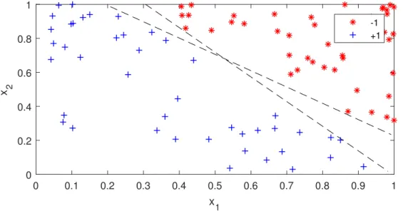
Figure 2.4: An example of data can be separated by infinite lines.
Figure 2.4 gives an example ofxi in Euclidean space with axisx1 and x2. In this situation, there are infinite hyperplanes that could separate all the training data. Hence, the learning algorithm stops when it finds the first line that satisfies the criteria in the training stage. However, the testing data are usually different from the training data. This results in some lines performing better than the others in the testing stage, despite all lines performing perfectly in the training stage.
2.1. Traditional Methods for Image Recognition 0 0.1 0.2 0.3 0.4 0.5 0.6 0.7 0.8 0.9 1 x 1 0.2 0.4 0.6 0.8 x 2 -1 +1 Support Vectors
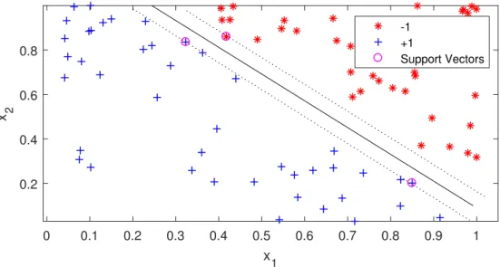
Figure 2.5: An example of the maximum margin in the SVM.
The key process in the SVM classifier is to find the hyperplane that separates the training data with the largest margin, as shown in Figure 2.5. The largest margin minimises the risk of making an error for the testing data, in other words, having a good generalisation ability [37]. If the training data is linearly separable, the two hyperplanes that guarantee the margin (dash lines in Figure 2.5) can be formulated as follows:
wTxi +b ≥+1, f or yi = +1, (2.8)
wTx
i +b ≤ −1, f or yi =−1, (2.9)
where w∈RM×1 and b are the weights vector and the bias, respectively. These two equations can also be combined into:
yi(wTxi+b)≥1, ∀i, (2.10)
where ∀i denotes for all i.
Considering the data lie on the hyperplane wTx
i +b = +1 in equation (2.8),
2.1. Traditional Methods for Image Recognition
Similarly, for data lying on the hyperplane wTx
i +b = −1 in equation (2.9), the
perpendicular distance between the hyperplane and the origin is|−1−b|/||w||2, where
|| · ||2 represent the l2-norm. Therefore, the margin between these two hyperplanes is 2/||w||2. The problem of finding the maximum margin 2/||w||2 equals to finding the minimum value of||w||2
2 subject to the constraints in equation (2.10), which can be formed as: min w,b 1 2||w|| 2 2, s.t. yi(wTxi+b)≥1, ∀i. (2.11)
The equation (2.11) can be interpreted in the Lagrangian formulation, which finds extrema for the functionf(x, y) given its constraints functiong(x, y) = 0. Similarly, in the SVM, function f(w) needs to be minimised given the inequality constraints functiong(w, b) = yi(wTxi+b)−1≥0. Therefore, the problem is solvable by using
the positive Lagrange multipliersαi, i= 1,· · ·, N, this gives the primal Lagrangian: LP = 1 2||w|| 2 2− N X i αiyi(wTxi+b−1) = 1 2||w|| 2 2− N X i αiyi(wTx+b) + N X i αi. (2.12)
Here LP must be minimised with respect to w and b without considering αi
first. Then it can be maximised afterw and b are substituted back, subject to the constraints that theαi ≥ 0. This is a convex quadratic programming problem [37]. LP is minimised by taking partial derivatives for w and b and setting them to 0:
∂LP ∂w =0 ⇒ w= N X i αiyixi, (2.13) ∂LP ∂b = 0 ⇒ b= N X i αiyi = 0. (2.14)
2.1. Traditional Methods for Image Recognition given: LD = 1 2w Tw−wT N X i αiyixi−b N X i αiyi+ N X i αi =−1 2w Tw+ N X i αi =−1 2 N X i N X j αiαjyiyjhxi,xji+ N X i αi, (2.15)
wherehxi,xjiis the inner product ofxi andxj. The solution is found by maximising LD subject to:
N
X
i
αiyi = 0, and αi ≥0, ∀i. (2.16)
This can be solved by the convex quadratic programming [37]. Notice that every training data xi is associated with a Lagrange multiplier αi. In the solution, most
values ofαi are zeros as they are far away from the margin hyperplane, which satisfy
either yi(wTxi +b) > 1 or yi(wTxi +b) < −1. Those xi with non-zero αi are the
support vectors. If the training data are not linearly separable, there are techniques that can either map the data into a linearly separable space by a kernel function or find a soft margin that is tolerant to some errors. This section gives an example of how a parameter classifier works and further reading about SVM can be found in [38]. In this example, the training process aims to find a fixed number of parameters in w and b. The learnedw and b can then be applied to classify testing data, with the training data being no longer required in the testing stage.
Non-parametric Classifier
For non-parametric approaches such asK Nearest Neighbours (KNN) [39], a testing data is compared with the entire training dataset. KNN is the simplest method for classification where a testing data is classified based on its nearest neighbours in the training dataset. Normally the Euclidean distance is used. When K = 1, the input
2.2. Deep Learning Framework for Image Recognition
point is assigned to the same class of its nearest neighbour. WhenK >1, the input point is assigned to the class that the majority of theseK nearest neighbours belong to. Easy implementation and good recognition results make KNN very popular for image classification [40–42].
Algorithm 2 The process of theKNN classification
1: For a testing data, calculate the Euclidean distance with all the training data. 2: Rank the distance from low to high and pick up the first K corresponding labels. 3: Find the majority vote from theK picked up labels and assign the label to the testing
data.
The KNN algorithm is an example of a non-parametric method that is often used for classification [43, 44]. However, a straightforward drawback of KNN is that the computational costs increase with the size of the training dataset. This is due to a testing data compared with all training data. Another drawback is that KNN algorithm is not stable in high dimension spaces [45]. This is because the shortest Euclidean distance is not necessarily the best match to the testing data, especially when the number of training data are limited [45, 46]. Besides, the
KNN algorithm has proven to be vulnerable to the effects of noise [47]. Meanwhile, the KNN algorithm gives an example that non-parametric classifiers do not need a training stage. While parametric classifiers might learn insufficient weights from the training stage, the non-parametric classifiers do not have this problem.
2.2
Deep Learning Framework for Image
Recog-nition
Traditional image recognition frameworks require image feature methods, followed by classification methods. There are plenty of methods and each method has pa-rameters that need to be defined by users. This raises the question: can we design a “black” box that takes images as the input and their corresponding labels as the output, without choosing image feature methods and classifiers? Neural networks
2.2. Deep Learning Framework for Image Recognition
are designed in this manner but the input reshapes an image to a vector. However, changing an image matrix to a vector loses the spatial information of the content, which is essential for images. Hence, the input of the “black” box should be a matrix in order to keep the spatial information at the beginning. The CNNs are designed to solve this problem. They use convolutional processes to preserve the spatial in-formation of the content; weights in the convolutional processes are automatically learned in a way similar to neural networks.
Lecun et al. proposed the first CNN framework LeNet [48]. Different CNN frameworks have been developed quickly after the AlexNet [1] achieved the best performance on ImageNet in 2012. Unlike neural networks, where neurons in each layer are fully connected to neurons in the next layer, each layer in a CNN shares the weights by using convolutional kernels. This process tremendously decreases the number of weights when compared with neural networks; therefore, it can prevent the over-fitting problem, which is one of the main problems in neural networks [49]. Another advantage is that the spatial information of the content is preserved by the convolutional process, while neural networks simply reshape an image into a vector, without preserving the spatial information. CNN frameworks are mainly composed of the convolution operations and the pooling operations. Figure 2.6 illustrates a typical CNN framework.
Figure 2.6: A typical CNN architecture example.
2.2. Deep Learning Framework for Image Recognition
kernels, which are equivalent to filters in the field of image processing. Kernels can be regarded as the shared weights connecting two layers. Suppose kernels of size [a×b×n] ([height×width×depth]) are used, theith (i= 1,2,· · · , n) convolutional
feature map can be denoted as:
Ci =f X j Vi∗ Ij ! , (2.17)
whereVi is the ith kernel and Ij (j = 1,2,· · · , J) is the jth feature map (Ij can be
a channel of the original image, a pooling map and a convolutional map). Heref(·) denotes a non-linear activation function and∗represents the convolutional operation. The Rectified Linear Unit (ReLU), where g(x) =max(0, x), is often applied as the non-linear function [1].
A convolutional process is often followed by a pooling process. In the pooling operation, a pooling process decreases the size of the input feature maps, which can be regarded as a down-sampling operation. Each pooling mapPi is usually obtained
by a pooling operation over the corresponding convolutional mapCi:
Pi =pool(Ci), (2.18)
where pool(·) represents a pooling method [50]. A window shifts on the previous mapCi and the mean value (or the maximum value) in each window is extracted in
order to form a pooling mapPi.
The convolution and pooling operations are the two main techniques in CNNs. As shown in Figure 2.6, these two processes are repeated. Note that convolutional processes are followed by pooling operations in Figure 2.6. However, this is not a requirement; different CNN structures are valid. Different CNN architectures have been developed rapidly subsequent to the AlexNet in 2012. For example, the ZF-Net [51] applied smaller kernel size in order to save more original pixel level information and achieved better results on ImageNet [52]. The VGG-NET [53] also enhanced the
2.3. Online Learning for Vehicle Logo Recognition
depth of the CNNs up to 19 layers and suggested only using a unique kernel size of [3×3]. The Google-Net [54] even increased the number of layers to 22 and applied the inception module, in which different convolutional feature maps (generated by convolutional kernels of different sizes) and the pooling feature maps were combined together. The Res-Net [55] built a 152 layer architecture and introduced the idea of the residual learning, which built short-cut connections between layers and achieved the best result on ImageNet in 2015.
It is found that the CNNs automatically learn simple structures of an image, such as edges in the initial convolutional layers, and more abstract information can be learned in later convolutional layers [51]. This is very similar to Hubel and Wiesel’s discovery [56] back in the 1960s, which suggests different orientation acti-vates different groups of neurons in the cat’s visual system. The CNNs have achieved great success and they currently dominate various image recognition tasks [57]. For example, face and motion recognition [58–60] and action recognition [61, 62].
2.3
Online Learning for Vehicle Logo Recognition
For the applications, this thesis start with the VLR problem, however, the developed methods can also be adapted to other image recognition tasks. VLR is important in Intelligent Transportation Systems (ITS) as the vehicle logo is one of the most distinguishable marks on a vehicle [63], and can assist in vehicle identification [43]. It has many potential applications in traffic monitoring and vehicle management systems. For instance, VLR can detect fraudulent plates if the combination does not match the data stored on the police security database [64]. As a result, this gives a more robust vehicle identification system. VLR could also provide guidance for autonomous driving systems and intelligent parking systems [65, 66]. In addi-tion, recognising vehicle logos is also useful for commercial investigations [67] and document retrieval [65].
2.3. Online Learning for Vehicle Logo Recognition
example, Rezaei and Farajzadeh [68] used the horizontal and vertical histograms to compare with a pre-defined template; it is, however, not robust to illuminations, noise and rotation variations. Sharpness histogram features [69] are used on well-segmented logo images. However, the accuracy is around 80%, which cannot make an effective recognition system. The Tchebichef moment invariants method is used on VLR but the computation costs are high [65, 70]. Peng [44] proposed a statistical random sparse distribution feature method which performs well in the low-resolution situation. The DenseSIFT is a global feature method that shares the same descrip-tion method with the SIFT descriptor while using every pixel as an interest point; this saves the computational costs for feature detection. However, it decreases the robustness of interest points. HOG [7] separates an image into small blocks and it calculates the horizontal gradients as well as vertical gradients in each block; it is a very successful global feature method and it is often used for VLR [7, 63, 71, 72].
However, local features are more favoured as they are robust to image noise, shift and rotations. For example, Yang [73] used the Harries corner detector to find the interest point for VLR. Psyllos et al. [43] and Lipikorn et al. [74] applied SIFT [2] features for vehicle logos. Badura and Foltan [75] used Speed Up Robust Features(SURF) [23] and achieved good results. Among local features, the SIFT feature method is the most popular on VLR [43, 74–76].
Currently CNN frameworks have been dominant in VLR, for instance, Gao and Lee [77] built a seven layer CNNs framework and achieved an accuracy of 88.4% on a self-selected dataset. Huang et al. [50] developed a pre-training process on CNNs for VLR, Xia et al. [78] created more images based on the dataset provided by [50] and developed a multi-task CNN framework for VLR. In general, CNN based methods are more accurate when there is a large training dataset. In the literature, transfer learning methods [79] have been developed, which fine tunes the weights based on the trained weight from big datasets in other domains. However, the automatic feature extraction method is particularly suitable for images from the source domain [79] .
2.4. Back-propagation Bayesian Compressive Sensing Classifier
In practice, there may only be an initially small training dataset, with additional images becoming available during the implementation. In order to take advantage of these additional images, new models can be built independently when more images become available. However, retraining new models increases the computational costs, especially when new models are updated frequently. CNNs update the weights online; however, it would not be useful in the earlier stage because training a CNN framework needs a huge dataset and involves huge computational costs. This motivates the work in Chapter 3, which develops a Cauchy prior LR framework for small dataset and CNNs are then applied when a big dataset becomes available.
2.4
Back-propagation Bayesian Compressive
Sens-ing Classifier
Parametric classifiers such as SVM and LR assume a functional distribution of the data [46]. Hence, the relationship between the label and the input data can be modelled using a fixed number of parameters. An advantage of parametric classi-fiers is that an increasing size of training dataset would not increase the number of parameters in the model. Therefore, the computational costs in the testing stage remain constant as classifying a testing data only needs these parameters. However, in practice, parametric classifiers can result in an inadequately trained model be-cause of inappropriate assumptions of prior distributions, leading to inappropriate predictions in the testing phase [33,46]. In contrast, non-parametric classifiers do not assume any particular distribution of the data, neither do they require a model with a fixed number of parameters [46]. In turn this increases the computational costs in the testing stage [80]. However, by avoiding models that can be insufficiently trained, they can be more flexible than the parametric classification methods [80].
A non-parametric classification approach based on sparse representation proposed by Wright et al. [81] has proved to be more accurate than the linear SVM and the
2.4. Back-propagation Bayesian Compressive Sensing Classifier
KNN classifier for face recognition. The SRC assumes that the testing data x∗ ∈
RM×1 can be represented as a linear combination of the training samplesX∈RM×N
where M is the length of the vector representing the data being considered and N
gives the number of entries in the training dataset. The linear representation of a testing image can be denoted as:
x∗ =Xw+z. (2.19)
In equation (2.19), w∈RN×1 is the weight vector that controls the contribution of each image in the training dataset to the linear combination representing the testing image, z ∈ RM×1 is a noise term with ||z||
2 6 and is a threshold constant. Conventionally, the solution ofw is often solved by choosing the minimum l2-norm distance:
ˆ
w= arg min w
(||w||2), s.t ||x∗−Xw||2 6. (2.20) where wˆ ∈ RN×1 is the estimated solution for the weight vector. However, the training dataset is often big enough to make N > M. Therefore, equation (2.19) represents an under-determined system and there is no unique solution by using conventional methods [81].
The SRC classification method assumes that a testing image can be sufficiently represented by instances from its corresponding class. Therefore, the solution is naturally sparse as coefficients for unrelated classes are zero valued. For instance, if there are 20 classes, only approximately 5% of the coefficients in wˆ will have non-zero values [81]. In fact, the sparser the recoveredwis, the easier it is to accurately classify the testing imagex∗ [81]. This motivates the use of thel0 to find the sparest solution forwin equation (2.19), wherel0 represents the number of non-zero entries.
minimisa-2.5. Image Restoration
tion is typically used as an approximation [82–84], giving:
ˆ
w= arg min w
(||w||1), s.t ||x∗−Xw||2 6. (2.21) The solution to thel1-norm minimisation in equation (2.21) can be solved by kernel reconstruction [85], or estimated by standard linear programming methods such as Basis Pursuit [86], greedy optimisation such as Orthogonal Matching Pursuit [87], and approximate kernel reconstruction method [88]. The solution of equation (2.19) gives the optimal w for classification purpose in the SRC [81].
Recently the Bayesian Compressive Sensing (BCS) [89] approach has been ef-ficiently applied to synthetic aperture radar target classification [90] and phonetic classification [91]. This Bayesian approach provides an alternative to the l1-norm minimisation for optimising the linear combination coefficients required for the clas-sification framework. Similar to Zhou et al. [92], by comparing the magnitudes of the coefficients, the testing data can then be classified by assigning it to the class whose coefficients have the highest l2-norm magnitude. Inspired by the Bayesian approach, this thesis proposes a back-propagation process based on BCS, which will be presented in Chapter 4.
2.5
Image Restoration
The image restoration process aims to recover a clear image from its corrupted ver-sion, including noise, rotation and occlusion. It is known as an ill-posed inverse prob-lem [93] and plenty of searches have been conducted in the literature. The majority of works are focused on single image de-noising and single image super-resolution. For example, total variation [94] and BM3D algorithm [95] achieved good perfor-mance in single image de-noising. [96–99] achieved a state-of-the-art perforperfor-mance on single image super-resolution [100]. However, these methods are only applicable for a particular image degradation. For example, BM3D is designed only for
im-2.5. Image Restoration
age de-noising. Deep learning based methods extract image features from groups of images and hence can be used for image de-noising and image super-resolution. In fact, deep neural network based methods take the advantage of the big data and the automatic learning scheme, and outperform the traditional image restoration meth-ods [93, 100]. Recently, the deep neural networks have been developed in order to solve different image restoration problems. For example, Mao et al. [93] proposed a CNN architecture that could perform image de-nosing and image super-resolution. The automatic learned restoration frameworks are more promising as they did not have any assumption about the degradation of the image, hence they are purely data driven [93]. Figure 2.7 shows the general structure of applying CNNs to image restoration similarly to [93].
Figure 2.7: A typical restoration architecture based on CNNs.
The restoration framework is based on the same convolutional operations as in CNNs. The main difference lies in there being no pooling operation and fully con-nected layers for restoration tasks. CNNs for recognition and restoration are different because recognition discards information layer by layer and ends up with a represen-tative feature vector (neurons in the last fully connected layer). In other words, the CNNs for classification discard information step by step in order to extract the most representative information of an image, while CNNs for restoration need to keep de-tailed information of the input image; hence, the pooling process is not appropriate. Image degradations also include image occlusion and image rotation. These problems are more challenging than image de-noising and image super-resolution, however, these problems are not well studied using state-of-the-art deep learning methods. This motivates the author to investigate the advanced image restoration methods dealing with image rotation and occlusion. In addition, it will be
ben-2.6. Summary
eficial if the recognition and restoration could share a joint network, which could perform both tasks at the same time, rather than in a pipeline manner (restoration followed by recognition). The author investigates these problems and develops joint frameworks for image recognition and image restoration. The joint frameworks could simultaneously perform image recognition and restoration with image degradations such as noise, rotation and occlusion. The related work will be presented in Chapter 5.
2.6
Summary
This chapter first introduces traditional recognition frameworks, which comprise im-age feature methods and classification methods. Among imim-age features, local feature methods such as SIFT features are more robust to image degradations than global feature methods such as HOG features. For the classifier, parametric and non-parametric classifiers are introduced with examples of SVM and KNN. The state-of-the-art recognition methods are shifting from traditional methods to the more advanced deep learning based methods such as CNNs. CNNs take advantage of the automatically learned features on big datasets and perform better than traditional methods in many application fields. However, CNNs contain many parameters that need big data and high computational costs to support. Considering the limitations of the CNNs, an online recognition for VLR is introduced, which will be extended to the proposed online Cauchy prior LR in Chapter 3. Considering the drawbacks for the non-parametric classifier such as KNN, this thesis develops a non-parametric classifier and this will be presented in Chapter 4. CNNs have also been applied for im-age restoration and classification separately in the literature, with imim-age restoration tasks particularity focused on image de-noising and image super-resolution. Hence, Chapter 5 considers image degradation including rotation and occlusion, and devel-ops deep learning based joint frameworks in order to simultaneously perform image recognition and restoration tasks.
Chapter 3
Online Learning for Vehicle Logo
Recognition
3.1
Introduction
Existing VLR frameworks train models on large fixed image training datasets. In practice, there may only be an initially small training dataset, with additional images becoming available during the implementation of the recognition scheme. In order to take advantage of these additional images, new models can be built independently when more images become available. However, retraining new models increases the computational costs, especially when new models are updated frequently. In order to deal with this problem, this chapter proposes a novel online framework for model learning, in which models are rebuilt efficiently using a weight updating scheme when dealing with datasets of an increasing size.
Figure 3.1: The developed framework of VLR with increasing size of dataset.
3.1. Introduction
small, the HOG features are applied for feature extraction and the online multinomial Cauchy prior LR classifier is applied for online model updating. The HOG algorithm is applied because of its efficiency. More importantly, it always gives the same feature vector for an image in any training stages. On the contrary, local feature methods involve a dynamic dictionary generation process, which results in different representation vectors for an image in different training stages. For example, using SIFT features with the BOW representation model, an image is represented by two different vectors when the training dataset contains 200 images and 500 images, respectively. In the parametric classification stage, weights are associated with the input vector. Therefore, if an image is represented by irrelevant vectors in different training stages, the corresponding weights will not be relevant. Hence, local features cannot be applied to the online weights updating scheme. Unlike local features requiring a representation model before the classification stage, the HOG algorithm does not need this process and it will always give the same vector despite different training scenarios. When large size datasets are available and high computational costs are acceptable, the CNN classifier can be applied in order to increase the robustness to noise and further improve the accuracy. Unlike hand-crafted features, which use fixed rules, features in CNNs automatically update according to more incoming data; hence, it could be more representative when there are more training images fed in.
For the choice of the classifier, LR can be easily extended for online model updat-ing and it explores the confidence level of the decision that the data has been correctly classified [33, 101]. However, when all training data can be perfectly classified, the LR suffers a common problem called separation, in which the maximum likelihood gives implausible estimates [102]. In order to have a generalised LR classifier without the separation problem, Gelman et al. [103] suggested a default Cauchy prior for LR and the posterior can be computed using Gibbs sampling, which involves high com-putational costs. This work combines the Conjugate Gradient Descent (CGD) with