Is Small Beautiful? Size Effects of Volatility Spillovers
for Firm Performance and Exchange Rates in Tourism*
Chia-Lin Chang
Department of Applied Economics Department of Finance
National Chung Hsing University, Taiwan
Hui-Kuang Hsu
Department of Finance and Banking National Pingtung Institute of Commerce, Taiwan
Michael McAleer
Econometric Institute Erasmus School of Economics Erasmus University Rotterdam
and
Tinbergen Institute, The Netherlands and
Institute of Economic Research Kyoto University, Japan
and
Department of Quantitative Economics Complutense University of Madrid, Spain
December 2012
* For financial support, the first author is most grateful to the National Science Council, Taiwan, and the third author wishes to acknowledge the Australian Research Council, National Science Council, Taiwan, and the Japan Society for the Promotion of Science.
Abstract
This paper examines the size effects of volatility spillovers for firm performance and
exchange rates with asymmetry in the Taiwan tourism industry. The analysis is based
on two conditional multivariate models, BEKK-AGARCH and VARMA-AGARCH,
in the volatility specification. Daily data from 1 July 2008 to 29 June 2012 for 999
firms are used, which covers the Global Financial Crisis. The empirical findings
indicate that there are size effects on volatility spillovers from the exchange rate to
firm performance. Specifically, the risk for firm size has different effects from the
three leading tourism sources to Taiwan, namely USA, Japan, and China. Furthermore,
all the return series reveal quite high volatility spillovers (at over sixty percent) with a
one-period lag. The empirical results show a negative correlation between exchange
rate returns and stock returns. However, the asymmetric effect of the shock is
ambiguous, owing to conflicts in the significance and signs of the asymmetry effect in
the two estimated multivariate GARCH models. The empirical findings provide
financial managers with a better understanding of how firm size is related to financial
performance, risk and portfolio management strategies that can be used in practice.
Keywords: Tourism, Size effects, Small-firm effects, Financial performance,
Spillover effects, MGARCH, VARMA, BEKK.
1. Introduction
Taiwan, just across the straits from mainland China, is the only island bisected by the Tropic of Cancer in East-Asia. Rich in tourism resources, Formosa, or “Beautiful Island”, is how the Portuguese viewed Taiwan when they sighted the untouched green island in the 16th Century. The majority of people in Taiwan widely speak Minnan (the Southern Chinese dialect) as many Taiwanese trace their lineage from the southern part of China. Two of the most popular foreign languages in Taiwan are Japanese and English, due to the Japanese occupation of Taiwan during 1895-1945, and the English curriculum for high school students.
From 2008 to 2011, approximately 5 million inbound tourists visited Taiwan annually. With close links in cultural exchange, bilateral trade and economic development, the leading inbound arrival sources to Taiwan are China, Japan, and USA, which account for over half (averaging nearly 54%) of inbound tourist arrivals annually during 2008-2011. In 2011, the growth of inbound visitors from these three leading tourist arrival sources was 9.41%, 19.87%, and 4.27% from China, Japan and the USA, respectively, as compared with the previous year.
The travel and tourism (T&T) sector, as a driver of economic growth, can stimulate GDP growth through jobs and enterprise creation, and provide significant foreign exchange revenues. The Government of Taiwan takes the tourism industry seriously, especially as the Global Financial Crisis of 2008-2009 severely cut Taiwan’s exports. In May 2009, the government proposed that the tourism industry is a core and bellwether industry among the six key emerging industries, namely biotechnology, green energy, high-end (high-quality) agriculture, medicine and health care, and cultural and creation industry, as the role of the tourism industry is to connect the six key emerging industries (for further details, see Tourism Bureau, Taiwan, 2011 tourism policies and the six emerging industries, respectively,
http://admin.taiwan.net.tw/public/public_en.aspx?no=6#T2011, http://www.cepd.gov.tw/encontent/m1.aspx?sNo=0011826).
A series of major investments in the tourism industry are expected to expand the tourism sector significantly, such asan amendment to the “Best of Taiwan Tourism Development Plan” in April 2009. The plan is intended to create about US$2,195 million in tourism revenues, add 437 thousand jobs, attract about US$833 million in private investment, and bring at least 10 major international hotel chains to Taiwan from 2009 through to 2013. Moreover, the government approved a constitutional
amendment to Tourism Policies in 2012, containing implementations of the “Project Vanguard for Excellence in Tourism (2009-2014)”, the “Medium-term Plan for Construction of Major Tourist Sites (2012-2015)”, and the “2012-2013 Tourism Promotional Focus” under the principles of sustainability, quality, amity, life, and diversity. These principles involve the advancement of balanced development of regional economies and tourism, and optimization of the lives of local residents and the quality of travel (http://admin.taiwan.net.tw/public/public_en.aspx?no=6). Above all, the Government of Taiwan regards the promotion of the tourism industry is high on the agenda.
The number of visitor arrivals exceeded 6 million in 2011, according to the Tourism Bureau in Taiwan. Visitor expenditures in Taiwan also experienced a rapid growth of 26.91% over the previous year. Historically, from 1991 to 2011, the visitor expenditure growth rate in Taiwan averaged 10.32%, reaching an all-time high of 27.92% in 2010, and a record low of -6.44% in 1997, excluding the 2002-2004 years of SARS in Asia. For the period 2008-2010, the growth in annual visitor expenditures in Taiwan was 13.85% in 2008, 14.82% in 2009, and 27.92% in 2010.
However, as the result of the Global Financial Crisis in 2009-2009, a still ongoing economic downturn, the economic uncertainty with high unemployment in Europe, Japan, and the USA has had adverse effects on the inbound tourism demand to Taiwan. Furthermore, in 2012, a series of new currency trading events occurred, such as direct trading of the Chinese Yuan against the Japanese Yen (on 1 June 2012), without using the U.S. dollar as an intermediate currency, other direct trade planning between the Chinese Yuan and Australian dollar, as well as the Chinese Yuan and New Taiwan dollar. Since 2008, China, the world’s second-largest economy ahead of Japan since 2010, has signed currency swap agreements with many countries, including the Republic of Korea and Malaysia. China’s agenda of gradually making the Chinese
Yuan a reserve currency has fostered trade tensions with the USA, and is expected to result in a significant impact on international money markets, especially in Asia.
However, little is known about volatility spillovers between exchange rate returns and firm performance in the tourism industry, especially a comparison of the spillovers according to firm size. Previous research has shown that exchange rates have a significant effect on the tourism market, especially on international tourist arrivals, tourism costs, tourism competition, firm’s earnings, relative purchasing power between the domestic and foreign countries, and the long term memory by tourists of such shocks over time.
As shown in previous research (see, for example, Becken et al., 2008; Blake et al., 2008), the exchange rate is an important factor of earnings for the tourism industry. Moreover, exchange rate fluctuations dominate the overall impact on the tourism price of the tourism industry over time. From the financial risk management perspective, organizing a portfolio management strategy will become more important for Taiwan tourism industry over time. In particular, the intensity of fluctuating impacts from exchange rates to the tourism industry might vary with the firm size. The primary purpose of the empirical section in this paper is to examine the performance of tourism firms as they relate to firm size.
For the breasons given above, it is worth exploring the information about risk spillovers from exchange rates to tourism performance, as well as examining how the tourism industry responds to changes in exchange rates for tourism industry firms of different sizes.
The remainder of the paper is organized as follows. Section 2 describes the data for analyzing size effects and spillover effects. Section 3 explains the data used in the empirical analysis, and the classification of tourism stock indexes by the trade markets. Section 4 discusses the methodology and models used to estimate the spillover effects. Section 5 presents the empirical results. Section 6 provides some concluding comments.
2. How to Evaluate the Spillover Effect and Size Effect
In this section we describe the spillover effect and size effect, as well as the proxies to be used to capture the magnitudes of these two effects.
2.1 Spillover Effect
The spillover effect refers to the interaction between two series. Traditional tourism demand models for international tourism demand suggests that tourism depends on exchange rates and other economic factors, such as the cost of airfares, incomes of tourists, and dummy variables(Dritsakis, 2004; Rossell et al., 2005). Tourism demand is negatively correlated with the exchange rate because tourists with higher purchasing power prefer to visit destinations with relatively lower purchasing power (Hanafiah and Harun, 2010). For example, the empirical findings for tourists from
Malaysia and New Zealand to Australia show that the memory of tourists of exchange rate shocks could diminish in the long run (Yap, 2011).
Chang and McAleer (2012)show that exchange rates are significant and have sensible interpretations for the time series of world, US and Japanese tourist arrivals to Taiwan, as well as world prices and two exchange rates, US$/New Taiwan $ and Yen/New Taiwan $, for tourist arrivals to Taiwan from the world, USA and Japan, and corresponding exchange rates. They also suggest that a strong domestic currency can have adverse effects on international tourist arrivals to Taiwan.
2.2 Size Effect of Firm Performance
As stated in Banz (1981), the common stock of small firms has, on average, higher risk-adjusted returns than that of large firms. This result will henceforth be referred to as the size effect, or small-firm effect. Firm performance may be driven by firm-specific factors, such as firm size. Several papers have shown that other factors may be more important to firm performance than firm-specific factors, such as demand, technological opportunity conditions, and industry effects (Cohen, 2010; Hansen and Wernerfelt, 1989; Hawawini et al., 2003; Mehran, 1995). Therefore, it is worth exploring the size effect on the performance of firms in the tourism industry, as well as for Taiwan, as there are many firm of different sizes involved in the tourism industry.
2.3 Proxy Variables for Firm Size and Firm Performance
In practice, stock returns are the most appropriate proxy of firm performance for all-equity firms (Mehran, 1995) because a firms’ stock price reflects the value of its future earnings, both from existing assets and their expected growth (Gay and Nam, 1998; Tufano, 1996). Several previous papers have indicated that a firm’s total assets (TA) can be taken as a proxy for firm size (Berger and Ofek, 1995; Zhou, 2003; Zimmerman, 1983). Therefore, this paper uses two proxies, namely stock index returns for firm performance, and trade market value of total assets (TA) for firm size (see Section 3 for further details) to explore the size effects on volatility spillovers between exchange rates and tourism firm performance. We will focus on the foreign currencies of the three leading international tourism sources to Taiwan, namely US Dollars, Japanese Yen, and Chinese Yuan.
3. Data
In this section we present the sampling, data grouping, and classifications of tourism stock indexes by the trade market, as related to firm size. Daily closing prices of foreign exchange rates and tourism stock indexes are used for 999 firms from 1 July 2008 to 29 June 2012, obtained from the databases of the Taiwan Stock Exchange (TWSE), Gre-Tai Securities Markets (GTSM), and the Taiwan Economic Journal (TEJ). The three foreign exchange rates associated with the three leading international tourism sources to Taiwan, namely USD/NTD, JNY/NTD, and CNY/NTD, are used in the empirical analysis.
Furthermore, as mentioned in Section 2.3, several previous papers have indicated that the firm’s total assets (TA) can be taken as a proxy for firm size. For capturing the size effect on olatility spillovers between exchange rates and firm performance, this paper classifies the tourism stock indexes into two categories, namely Large and Small, by the trade market (a proxy for firm size), which varies according to the requirements of paid-in capital when a public issuer applies for listing.
Therefore, the tourism-related firms listed on the market of the Taiwan Stock Exchange (TWSE) are defined as large firms (that is, Large), whereas the tourism-related firms listed on the Gre-Tai Securities Market are regarded as small firms (that is, Small). The requirement of a firm’s paid-in capital for listing on the Taiwan Stock Exchange is at least NT$600 million, which is greater than for the Gre-Tai Securities Market, which is at least NT$50 million, at the time a public issuer applies for listing.
4. Multivariate Conditional Volatility Models for Spillover Effects
Caporin and McAleer (2012) note that the two most widely-used models of conditional covariance and correlation in the class of multivariate GARCH models are BEKK (see Baba, Engle, Kraft and Kroner, 1995); Engle and Kroner, 1995) and Dynamic Conditional Correlation (DCC) (see Engle, 2002). In addition to estimating conditional covariances consistently, the BEKK model can also be used to obtain consistent estimates of dynamic conditional correlations, with a direct link to the indirect DCC model (Caporin and McAleer, 2008).
in the conditional covariance specification. Therefore, taking account of the volatility transmission effects across different markets and assets (specifically, exchange rate returns and stock index returns), together with the asymmetric effect, this paper adopts the VARMA-AGARCH model originally proposed by Ling and McAleer (2003) and extended in McAleer et al. (2009). This specification nests the univariate asymmetric GJR model of Glosten, Jagannathan and Runkle (1993) in modelling the conditional variance process.
The following are the model specifications of the conditional mean and the conditional covariances.
4.1Specification of the Conditional Mean
The multivariate GARCH model is developed to examine the joint processes relating the returns of several different series. As mentioned above, there are two series in each portfolio in this paper, namely exchange rate returns and stock index returns.
The following conditional expected returns equation at time t accommodates each variable’s own past returns at time t-1 and the returns of other variables that are lagged one period:
; (4.1)
where is an vector of daily returns at time t for each returns series (in this case, = 2 for exchange rate returns and stock index returns), and . The vector of random errors represents the shocks for each series at time t, with corresponding conditional covariance matrix . The market information available at time t-1is represented by the information set, . The vector, , represents the long-term drift coefficients.
The estimates of the elements of the coefficient matrix, , enable us to measure the effects of the impacts on the mean returns of one series arising from its own past returns and the lagged returns of the other series.
4.2 BEKK Specification of the Conditional Variance
The BEKK formulation of Baba et al. (1985) and Engle and Kroner (1995) directly imposes positive definiteness on the conditional variance matrix. Specifically, in order
to capture the asymmetric effects of shocks on conditional volatility, this paper uses the GJR specification of the multivariate GARCH model and includes an indicator variable for negative returns shocks. The BEKK model for multivariate GARCH (1,1) with asymmetry, which nests the GJR model, is given as:
(4.2)
where
The diagonal elements in the parameter matrix, B, measure the own-effects of lagged volatility, while the off-diagonal elements capture the cross-market effects. The asymmetry terms are labelled as D. Positive parameter estimates in D in the context of a univariate GJR model suggest that negative shocks to returns subsequently lead to a higher conditional variance in the following, than do positive shocks of equal magnitude. The matrix of conditional covariances in equation (4.2) is positive definite, by construction, this attractive aspect of the BEKK specification comes at the cost of over-parameterization, otherwise known as the curse of dimensionality.
With all the parameters entering through quadratic forms, changing the signs of all the elements of W, A, or B will have no effect on the conditional covariance. The stationarity condition is given by . Furthermore, we need
have only free parameters as the BEKK specification is parameterized to be lower triangular. The parameters of the model are obtained by maximum likelihood estimation (MLE) using a joint normal density function. When the matrix of returns shocks does not follow a joint multivariate normal distribution, the appropriate method is to use quasi-maximum likelihood estimation (QMLE) (for further details, see Chang, McAleer and Tansuchat, 2011).
4.3 VARMA-GARCH Specification of the Conditional Variance
The VARMA-GARCH model proposed by Ling and McAleer (2003), a vector autoregressive moving average specification, incorporates volatility transmission effects across different markets and assets under the assumption that negative and positive shocks of equal magnitude have identical impacts on the conditional variance. However, it is unrealistic to assume that the impacts on the conditional variance from negative and positive shocks of equal magnitude are identical.
In order to capture the asymmetric property of differential impacts on the conditional variance arising from negative and positive shocks of equal magnitude, McAleer et al. (2009) extended the VARMA-GARCH model to accommodate the asymmetric impacts of the unconditional shocks on the conditional variance, and proposed the VARMA-AGARCH specification of the conditional variance. The vector ARMA-AGARCH model accommodates interdependencies in the conditional volatilities with asymmetric impacts of the unconditional shocks on the conditional variances across different assets and/or markets
The VARMA-AGARCH model is given as follows:
where are m× m matrices for i=1,.., r, with typical element , and
is an indicator function, given as
The specification of the VARMA-AGARCH (1,1) in this paper is given as follows:
where are 2 × 2 matrices with typical element , and is an indicator function. This allows large shocks in one variable to affect the conditional variances of the other variables. Furthermore, VARMA-AGARCH reduces to VARMA-GARCH when . In Ling and McAleer (2003) and McAleer et al. (2009), the structural and statistical properties of the model are explained in detail, including the necessary and sufficient conditions for stationarity and ergodicity of both VARMA-GARCH and VARMA-AGARCH.
The parameters of the model are obtained by maximum likelihood estimation (MLE) using a joint normal density. When does not follow a joint multivariate normal distribution, the appropriate estimator is QMLE (for example, see Chang et al., 2011). This paper adopts the VARMA-AGARCH model proposed by Ling and McAleer (2009) and McAleer et al. (2009) to model the conditional covariances simultaneously for capturing the properties of asymmetric effects and volatility spillovers among the vector of different assets.
5. Empirical Results
This paper examines the size effects on volatility spillovers with asymmetry between the exchange rate returns and stock index returns (which are a proxy for firm performance) using two multivariate conditional covariance models, namely BEKK-AGARCH (1,1) and VARMA-AGARCH (1,1), for modelling the conditional covariance process. The empirical findings of the six portfolios are discussed below.
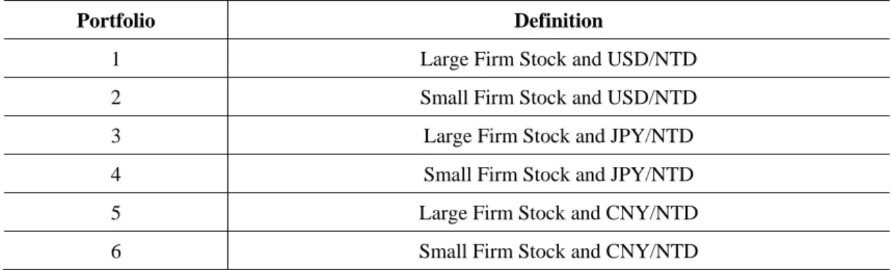
First, we calculate exchange rates returns and tourism stock index returns as the first difference in log prices, defined as , where and are the daily closing prices at time periods t and t-1, respectively. Table 1 shows the operational definitions of the log return series used in the paper. Moreover, for examining the size effects on the volatility transmission between the two series, this paper uses five returns series (namely three exchange rate returns and two stock index returns) into six portfolios according to currency and firm size, namely Portfolio 1 (USD/NTD with Large Firms), Portfolio 2 (USD/NTD with Small Firms), Portfolio 3 (JPY/NTD with Large Firms), Portfolio 4 (JPY/NTD with Small Firms), Portfolio 5 (CNY/NTD with Large Firms), and Portfolio 6 (CNY/NTD with Small Firms). As shown as Tables 2 and 3, based on the negative correlation of two specific series, this implies greater diversification benefits arising from a portfolio (Bodie, 1976).
[Tables 1-3 here]
5.1 Graphs and Descriptive Statistics of Returns
This paper examines the time series data graphically. Figures 1 to 3 plot the trends, logarithms, and log differences (that is, the growth rate or the continuously compounded returns) of five data series. Figures 4 to 9 plot the time varying correlations of Portfolio 1 to 6. Moreover, Table 4 presents the basic descriptive statistics for the five returns series. In terms of exchange rate returns, the average returns of USD/NTD are negative and very low, whereas the average returns of JPY/NTD and CNY/NTD are positive and low. However, both means of the stock returns series (namely Large Firms and Small Firms) have negative and low values.
[Figures 1-9 here] [Table 4 here]
behavior, as evidenced by large kurtosis with respect to the Gaussian distribution. In addition, four of the five series show mild positive skewness, with only Large Firms being negatively skewed. The negative skewness statistic implies the series has a shorter right tail than left tail. The Jarque-Bera Lagrange multiplier test statistics indicate that none of these return series is normally distributed, which is not at all surprising for returns data.
5.1Unit Root Test of Returns
A unit root test examines whether a time series variable is non-stationary. Two well-known tests, the GLS-detrended Dickey-Fuller test and the Phillips-Perron (PP) test, are calculated to test for unit root processes. The results of the unit root tests are shown in Table 5 and indicate that all returns series are stationary. The unit root tests for each individual returns series reject the null hypothesis of a unit root at the 1% level of significance.
[Table 5 here]
5.2Results of Six Portfolios with BEKK
All the returns series examined in Table 6 reveal quite high volatility spillovers (in excess of eighty percent) from its own lags, and are given as and . On the other hand, as the BEKK specification states, the off-diagonal elements of the matrix
B measure the cross-market effects, or the volatility spillover effects between the series. According to the empirical findings from Portfolio 3, for instance, the volatility from exchange returns (JPY/NTD) to large stock index returns (Large Firms), , is 34.09%, but the reverse effect (in absolute value), , is only 2.56%. This implies that the volatility spillover from exchange rate returns is much stronger than from stock index returns (firm performance).
[Table 6 here]
As noted in Section 4.2 of the BEKK specification, the significant and positive coefficient, γ, or asymmetry, indicates that negative shocks tend to produce higher volatility in the following period than do positive shocks of a similar magnitude. Table 6 indicates that some of the estimates confirm the evidence of asymmetry, shown as γ. For instance, in Portfolios 2, 4 and 6, the previous shock transmission from the small stock index returns (Small Firms) affect all the exchange rate returns
(USD/NTD, JPY/NTD, and CNY/NTD), shown as , but the reverse does not hold from exchange rate returns to small stock index returns.
As , the individual stationarity conditions of the estimates
for all the returns series given in Table 6 are satisfied.
5.3Results of Six Portfolios with VARMA-AGARCH
All the return series examined in Table 7 reveal quite high volatility spillovers (of over sixty percent) from its own lags, and shown as and . Followed by the interdependence of volatility spillovers transmitted across markets, the results in Table 7 indicate that there is a significant finding on the returns of large firm stock indexes (Large Firms) associated with both exchange rate returns (USD/NTD and CNY/NTD), whereas the returns of small stock indexes (Small Firms) only affect one set of exchange rate returns (JPY/NTD). This implies that there is a size effect on the risk interdependence from exchange rate returns to stock index returns (firm performance) for the tourism stock market in Taiwan. Such an empirical finding arises because the risk associated with each firm size has different transmissions from the three leading international tourism sources to Taiwan.
[Table 7 here]
Referring to Section 4.1, the univariate GJR model is a simple extension of univariate GARCH with an additional term to account for asymmetry. The significant and positive coefficient, γ, indicates that negative shocks tend to produce higher volatility in the following period than do positive shocks of a similar magnitude. According to the estimates in Table 7, shown as γ, all the returns of large stock indexes (Large Firms) confirm the presence of asymmetry, whereas none of the returns of small stock indexes (Small Firms) suggest asymmetry.
As the stationarity condition (a + b < 1) is satisfied for each returns series examined in Table 7, all the returns series satisfy the second moment and log-moment conditions, which are sufficient conditions for the Quasi-Maximum Likelihood Estimator (QMLE) to be consistent and asymptotically normal (for further details, see (McAleer, Chan and Marinova, 2007). Therefore, it is valid to conduct standard statistical inference.
This paper examined the size effects on volatility spillovers between exchange rate returns and tourism performance with asymmetry for the Taiwan tourism industry, using two proxies, namely the trade market for firm size (Large Firms and Small Firms) and stock index returns for firm performance.
We used two multivariate conditional volatility models, namely BEKK and VARMA_AGARCH, for modelling the conditional covariance process, using daily log returns data, including exchange rate returns (USD/NTD, JPY/NTD, and CNY/NTD) and tourism stock index returns (Large Firms and Small Firms) for the period 1 July 2008 to 29 June 2012.
The empirical findings revealed that there was a negative correlation between exchange rate returns and stock index returns, implying greater diversification benefits as a portfolio. All the returns series examined showed quite high volatility spillovers (of over sixty percent) from its own effects in the previous period.
Furthermore, the empirical findings indicated that there were size effects on volatility spillovers from the exchange rate to firm performance because the risk for each firm size had different transmissions from the three leading international tourism sources to Taiwan, namely the USA, Japan and China. For large tourism index returns, there were volatility spillover effects transmitted from two exchange rate returns (USD/NTD and CNY/NTD), whereas there were volatility spillover effects only from exchange rate returns of Japanese Yen (JPY/NTD) for small tourism index returns.
Overall, the asymmetric effects of shocks for the tourism industry in Taiwan are ambiguous arising from conflicts in the statistical significance and signs of the asymmetric term estimated in the two multivariate conditional volatility models.
In summary, this paper explained the size effects on volatility spillovers between the exchange rate and tourism performance, as well as the negative correlation between the two returns series, implying greater diversification benefits as a portfolio. Moreover, the empirical findings can provide financial managers with a better understanding of how firm size is related to financial performance, risk and portfolio management strategies that can be used in practice.
References
Baba, Y., Engle, R.F., Kraft, D., and Kroner, K.F. (1989), Multivariate simultaneous generalized ARCH, Unpublished manuscript, Department of Economics, University of California, San Diego.
Banz, R.W. (1981), The relationship between return and market value of common stocks, Journal of Financial Economics, 9(1), 3-18.
Becken, S., Carboni, A., Vuletich, S., and Schiff, A. (2008), Analysis of tourist consumption, expenditure and prices for key international visitor segments, Technical Report.
Berger, P.G., and Ofek, E. (1995), Diversification's effect on firm value, Journal of Financial Economics, 37(1), 39-65.
Blake, A., Arbache, J.S., Sinclair, M.T., and Teles, V. (2008), Tourism and poverty relief, Annals of Tourism Research, 35(1), 107-126.
Bodie, Z. (1976), Common stocks as a hedge against inflation, Journal of Finance, 31(2), 459-470.
Caporin, M., and McAleer, M. (2008), Scalar BEKK and indirect DCC, Journal of Forecasting, 27, 537-549.
Caporin, M., and McAleer M. (2012), Do we really need both BEKK and DCC? A tale of two multivariate GARCH models, Journal of Economic Surveys, 26(4), 736-751.
Chang, C., and McAleer, M. (2012), Aggregation, heterogeneous autoregression and volatility of daily international tourist arrivals and exchange rates”, Japanese Economic Review, 63(3), 397-419.
Chang, C.L., McAleer, M., and Tansuchat, R. (2011), Crude oil hedging strategies using dynamic multivariate GARCH, Energy Economics, 33(5), 912-923.
Cohen, W.M. (2010), Fifty years of empirical studies of innovative activity and performance, Handbook of the Economics of Innovation, 1, 129-213.
Dritsakis, N. (2004), Cointegration analysis of German and British tourism demand for Greece, Tourism Management, 25(1), 111-119.
Engle, R. (2002), Dynamic conditional correlation: A simple class of multivariate generalized autoregressive conditional heteroskedasticity models, Journal of Business and Economic Statistics, 20(3), 339-350.
Engle, R.F., and Kroner, K.F. (1995), Multivariate simultaneous generalized ARCH, Econometric Theory, 11(1), 122-150.
Gay, G.D., and Nam, J. (1998), The underinvestment problem and corporate derivatives use, Financial Management, 53-69.
Glosten, L.R., Jagannathan, R., and Runkle, D.E. (1993)., On the relation between the expected value and the volatility of the nominal excess return on stocks, Journal of Finance, 48(5), 1779-1801.
Hanafiah, M.H.M., and Harun, M.F.M. (2010), Tourism demand in Malaysia: A cross-sectional pool time-series analysis, International Journal of Trade, Economics, and Finance, 1(1), 80-83.
Hansen, G.S., and Wernerfelt, B. (1989), Determinants of firm performance: The relative importance of economic and organizational factors, Strategic Management Journal, 10(5), 399-411.
Hawawini, G., Subramanian, V., and Verdin, P. (2003), Is performance driven by industry‐or firm‐specific factors? A new look at the evidence, Strategic Management Journal, 24(1), 1-16.
Ling, S., and McAleer, M. (2003), Asymptotic theory for a vector ARMA-GARCH model, Econometric Theory, 19, 278-308.
McAleer, M., Chan, F., and Marinova, D. (2007), An econometric analysis of asymmetric volatility: Theory and application to patents, Journal of Econometrics, 139(2), 259-284.
multivariate asymmetric conditional volatility, Econometric Reviews, 28(5), 422-440.
Mehran, H. (1995), Executive compensation structure, ownership, and firm performance, Journal of Financial Economics, 38(2), 163-184.
Rossell, J., Aguil, E., and Riera, A. (2005), Modeling tourism demand dynamics, Journal of Travel Research, 44(1), 111-116.
Tufano, P. (1996), Who manages risk? An empirical examination of risk management practices in the gold mining industry, Journal of Finance, 51(4), 1097-1137.
Yap, G. (2011), Modelling the spillover effects of exchange rates on Australia's inbound tourism growth. Available at SSRN 1789645.
Zhou, X. (2003), CEO pay, firm size, and corporate performance: Evidence from Canada, Canadian Journal of Economics, 33(1), 213-251.
Zimmerman, J.L. (1983), Taxes and firm size, Journal of Accounting and Economics, 5, 119-149.
Figure 1
Time Series Plots of Daily Closing Prices
(a) Large Firm
50 100150200250300350400450500550600650700750800850900950 40 120 (b) Small Firm Firm 50 100150200250300350400450500550600650700750800850900950 80 140 200 (c) USD 50 100150200250300350400450500550600650700750800850900950 28 32 36 (d) JPY 50 100150200250300350400450500550600650700750800850900950 0.28 0.36 (e) CNY 50 100150200250300350400450500550600650700750800850900950 4.4 4.8 5.2
Figure 2
Time Series Plots for Log Daily Closing Prices (a) logLarge 50 100150200250300350400450500550600650700750800850900950 400 460 520 (b) logSmall 50 100150200250300350400450500550600650700750800850900950 420 480 540 (c) logUSD 50 100150200250300350400450500550600650700750800850900950 335.0 345.0 355.0 (d) logJPY 50 100150200250300350400450500550600650700750800850900950 -130 -110 -90 (e) logCNY 50 100150200250300350400450500550600650700750800850900950 148 156 164
Figure 3
Time Series Plots for Daily Returns
(a) Large Firm
50100150200250300350400450500550600650700750800850900950 -7.5 0.0 7.5 (b) Small Firm 50100150200250300350400450500550600650700750800850900950 -7.5 0.0 7.5 (c) USD/NTD 50100150200250300350400450500550600650700750800850900950 -2.0 0.0 (d) JPY/NTD 50100150200250300350400450500550600650700750800850900950 -4 0 (e) CNY/NTD 50100150200250300350400450500550600650700750800850900950 -2.5 -0.5 1.5
Figure 4
Correlation of Large Firms with USD/NTD in Portfolio 1
Figure 5
Correlation of Small Firms with USD/NTD in Portfolio 2
100 200 300 400 500 600 700 800 900 -0.6 -0.5 -0.4 -0.3 -0.2 -0.1 -0.0 0.1 100 200 300 400 500 600 700 800 900 -0.6 -0.5 -0.4 -0.3 -0.2 -0.1 -0.0 0.1 0.2
Figure 6
Correlation of Large Firms with JPY/NTD in Portfolio 3
Figure 7
Correlation of Small Firms with JPY/NTD in Portfolio 4
100 200 300 400 500 600 700 800 900 -0.42 -0.40 -0.38 -0.36 -0.34 -0.32 -0.30 -0.28 -0.26 -0.24 100 200 300 400 500 600 700 800 900 -0.375 -0.350 -0.325 -0.300 -0.275 -0.250
Figure 8
Correlation of Large Firms with CNY/NTD in Portfolio 5
Figure 9
Correlation of Small Firms with CNY/NTD in Portfolio 6
100 200 300 400 500 600 700 800 900 -0.5 -0.4 -0.3 -0.2 -0.1 -0.0 0.1 100 200 300 400 500 600 700 800 900 -0.40 -0.35 -0.30 -0.25 -0.20 -0.15 -0.10 -0.05 -0.00
Table 1
Definitions of Variables of Stocks Indexes and Exchange Rates
Variables Definition
R 1
Stock indexes
Large Firms Returns of tourism indexes listed on the Taiwan Stock Exchange (TWSE) for large firms
Small Firms Returns of tourism indexes listed on Taiwan Gre-Tai Securities Markets (GTSM) for small firms
R2
Exchange rates
USD/NTD Returns of changes in daily closing prices of the exchange rate of the New Taiwan Dollar to the US Dollar
JPY/NTD Returns of changes in daily closing prices of the exchange rate of the New Taiwan Dollar to the Japanese Yen
CNY/NTD Returns of changes in daily closing prices of the exchange rate of the New Taiwan Dollar to the Chinese Yuan (Renminbi)
Table 2 Six Portfolios
Portfolio Definition
1 Large Firm Stock and USD/NTD
2 Small Firm Stock and USD/NTD
3 Large Firm Stock and JPY/NTD
4 Small Firm Stock and JPY/NTD
5 Large Firm Stock and CNY/NTD
6 Small Firm Stock and CNY/NTD
Table 3
Correlation Coefficients for Stock Indexes and Exchange Rates
( ) Portfolio 1 Portfolio 2 Portfolio 3 Portfolio 4 Portfolio 5 Portfolio 6
R 1 Large Firm Small Firm Large Firm Small Firm Large Firm Small Firm
R2 USD/NTD USD/NTD JPY/NTD JPY/NTD CNY/NTD CNY/NTD
-0.2833 -0.2232 -0.2804 -0.2878 -0.203 -0.1879
Notes:
(1) : Stock indexes (Large Firms and Small Firms)
: Exchange rates (USD/NTD, JPY/NTD, and CNY/NTD) (2) : Correlation coefficient of R 1 and R2
Table 4
Descriptive Statistics (2008/07/01 – 2012/06/29)
R 1 R2
Returns Large Firms Small Firms USD/NTD JPY/NTD CNY/NTD
Mean -0.0067 -0.0414 -0.0016 0.0271 0.0054 Median -0.0511 -0.0716 0.0000 0.0287 0.0000 Maximum 6.7304 6.6763 1.4398 2.9870 1.9211 Minimum -7.1714 -7.1461 -1.5875 -3.6274 -2.1323 Std. Dev. 2.2361 2.2309 0.2843 0.8241 0.3371 Skewness 0.0447 -0.0172 -0.1217 -0.1799 -0.1031 Kurtosis 4.3823 4.1765 6.6431 5.1847 8.6004 Jarque-Bera 79.79 57.61 554.37 203.86 1306.00 Prob-value 0 0 0 0 0 Sum -6.7162 -41.3136 -1.5417 27.000 5.3928 Sum Sq. Dev. 4985.114 4961.832 80.59974 677.074 113.299 Observations 998 998 998 998 998
Table 5
Unit Root Tests (2008/07/01 – 2012/06/29)
Variables ADF (GLS) PP (Phillips-Perron)
R 1 Large Firms -4.780655*** -26.64180*** Small Firms -26.54002*** -27.16912*** R2 USD/NTD -18.17521*** -28.17543*** JPY/NTD -32.78753*** -33.02619*** CNY/NTD -34.23034*** -34.33451*** Note:
1. *** denotes the null hypothesis of a unit root is rejected at the 1% level. 2. ** denotes the null hypothesis of a unit root is rejected at the 5% level. 3. * denotes the null hypothesis of a unit root is rejected at the 10% level.
Test critical values: 1% : -3.43683 ; 5% : -2.86429 ; 10% : -2.568286 4. Stock Index Returns: Large and Small
Table 6
Spillovers between Stock Returns and Exchange Rate Returns for BEKK-AGARCH
Portfolio 1 Portfolio 2 Portfolio 3 Portfolio 4 Portfolio 5 Portfolio 6
R1,t Large Firm Small Firm Large Firm Small Firm Large Firm Small Firm
R2,t USD/NTD JPY/NTD CNY/NTD
Coefficient Mean Equation Mean Equation Mean Equation
-0.0433 -0.0373 -0.0394 -0.04995 -0.05116 -0.04204 0.0877 0.0829 0.0925 0.09237 0.10247 0.09052 -0578 -0.7884 -0.0618 0.00525 -0.13450 -0.42068 -0.0090 -0.0057 0.0084 0.00300 -0.00093 0.00137 0.1231 0.1441 -0.0263 -0.03526 -0.02786 -0.01757 0.0057 0.0079 0.0106 0.01175 0.00568 0.00691
Coefficient Variances Equation Variances Equation Variances Equation
-0.3142 0.2101 0.0000 0.0883 0.2213 0.2526 01837 -0.0709 -0.2891 -0.1279 0.1440 -0.0326 0.0511 0.0688 0.1865 0.1304 0.0848 0.1017 0.2051 0.1855 0.1044 0.1402 0.1322 0.1932 0.0132 -0.0030 0.0567 0.0431 0.0196 -0.0077 0.3090 -0.0780 -0.5286 -0.3279 0.4132 0.1155 0.3871 0.3853 0.2402 0.2206 0.3713 0.3556 0.9176 0.9706 0.9430 0.9801 0.9338 0.9544 -0.0069 0.0003 -0.0255 -0.0194 -0.0050 0.0022 -0.3294 0.0201 0.3408 0.1967 -0.4283 -0.2114 0.8812 0.8634 0.9077 0.9347 0.8668 0.8382 0.3618 -0.1495 0.3927 -0.1871 -0.3503 -0.2115 -0.0002 0.0149 -0.0673 0.0791 0.0045 0.0166 -0.6705 0.1300 -0.1623 -0.1593 0.6341 0.3651 -0.2995 0.3311 -0.1060 -0.0795 0.3032 0.3931 Notes:
(1) Entries in bold are significant at the 5% level.
Table 7
Spillovers between Stock Returns and Exchange Rate Returns for VARMA-AGARCH
Portfolio 1 Portfolio 2 Portfolio 3 Portfolio 4 Portfolio 5 Portfolio 6
R1,t Large Firm Small Firm Large Firm Small Firm Large Firm Small Firm
R2,t USD/NTD JPY/NTD CNY/NTD
Coefficient Mean Equation Mean Equation Mean Equation
-0.0413 -0.0507 -0.0669 -0.0223 -0.0377 -0.0587 0.0988 0.0818 0.0927 0.1126 0.1240 0.0962 -0.5788 -0.8592 0.0080 0.0274 -0.2630 -0.5052 -0.0086 -0.0071 0.0171 0.0080 0.0021 0.0031 0.1066 0.1333 -0.0790 -0.0576 -0.0490 -0.0262 0.0036 0.0072 0.0080 0.0082 0.0051 0.0066
Coefficient Variances Equation Variances Equation Variances Equation
0.0342 0.0362 0.1511 0.0301 -0.0045 0.0156 0.0008 0.0010 0.0058 0.0066 0.0038 0.0070 0.0280 0.0420 0.0233 0.0377 0.0092 0.0314 0.3359 0.2302 -0.0080 0.0203 0.1566 0.1767 0.0186 0.0124 -0.0142 -0.0097 0.0251 0.0072 0.1781 0.1833 0.0431 0.0639 0.1647 0.1594 0.8678 0.9242 0.7296 0.9482 0.9219 0.9221 -0.0636 -0.0894 0.0212 -0.0968 -0.1202 -0.0721 -1.6555 -0.7433 -1.1670 -0.0853 -1.4734 -1.1231 0.7292 0.6663 0.9821 0.8753 0.7010 0.6731 0.0925 0.0166 0.1784 -0.0034 0.0573 0.0284 0.0274 0.0900 -0.0573 -0.0615 -0.0143 0.0850 Notes:
(1) Entries in bold are significant at the 5% level.