Doktor der Ingenieurwissenschaften (Dr.-Ing.) der Landwirtschaftlichen Fakultät
der Rheinischen Friedrich-Wilhelms-Universität Bonn Institut für Geodäsie und Geoinformation
Robot Mapping and Navigation
in Real-World Environments
von
Igor Bogoslavskyi
ausReferent:
Prof. Dr. Cyrill Stachniss, Friedrich-Wilhelms-Universität Bonn
1. Korreferent:
Prof. Dr. Giorgio Grisetti, La Sapienza University of Rome
2. Korreferent:
Prof. Dr. Wolf-Dieter Schuh, Friedrich-Wilhelms-Universität Bonn
Tag der mündlichen Prüfung: 19. November 2018
Erscheinungsjahr: 2018
Ich erkläre hiermit an Eides statt, dass ich die vorliegende Arbeit ohne Hilfe Dritter und ohne Benutzung anderer als der angegebenenen Hilfsmittel angefer-tigt habe; die aus fremdem Quellen direkt oder indirekt übernommenen Gedanken sind als solche kenntlich gemacht. Die Arbeit wurde bisher in gleicher oder ähn-licher Form in keiner anderen Prüfungsbehörde vorgelegt und auch noch nicht veröffentlicht.
R
oboterkönnen unterschiedlichste Aufgaben ausführen, z.B. in Such-und Rettungsszenarien eingesetzt werden, Waren ausliefern oder Per-sonen transportieren. Roboter, die in der realen Welt eingesetzt wer-den, müssen viele Herausforderungen auf dem Weg zur Vollendung ihrer Mission meistern. Zentrale Fähigkeiten, die für den Betrieb solcher Roboter erforderlich sind, sind Kartierung, Lokalisierung und Navigation. Die robuste Lösung dieser Aufgaben ist eine nicht-triviale Aufgabe, da unter anderem die Komponenten typischerweise voneinander abhängig sind. So muss beispielsweise ein Roboter gleichzeitig eine Karte aufbauen, sich darin lokalisieren, die Umge-bung bzgl. möglichen Kollisionen analysieren und einen geeigneten Weg planen, um eine unbekannte Umgebung effizient zu erkunden.Die Lösungen dieser Aufgaben hängen meist von den verwendeten Sensoren und von der Art der Einsatzumgebung ab. Eine RGB-Kamera kann zum Beispiel in einer Außenszene zum Berechnen einer visuellen Odometrie oder zur Erken-nung dynamischer Objekte verwendet werden. Im Gegensatz dazu ist sie weniger nützlich in Umgebungen, die nicht genug Licht für den Betrieb von Kameras zur Verfügung stellen. Des Weiteren sollte die Software, die das Verhalten des Robot-ers steuert, alle Daten der vRobot-erschiedenen Sensoren verarbeiten und integrieren. Dies führt oft zu technischen Systemen, die nur mit einem bestimmten Robotertyp und einem bestimmten Satz von Sensoren funktionieren. In dieser Doktorarbeit fokussieren wir uns auf Systeme und implementieren Methoden für Roboternavi-gationssysteme, die nahtlos mit verschiedenen Sensoren arbeiten können, sowohl im Innen- als auch im Außenbereich. Speziell mit der kürzlichen Entwicklung neuer distanzmessender RGBD und LiDAR Sensoren sehen wir die Möglichkeit Systeme zu bauen, die sowohl im Innen- als auch im Außenbereich robust arbeiten können und erweitern, damit die Einsatzgebiete von mobilen Robotern.
Die in dieser Arbeit vorgestellten Techniken zielen darauf ab, sowohl mit RGBD als auch mit LiDAR Sensoren – ohne Anpassungen für einzelne Sensor-modelle – Methoden für Navigation und Szeneninterpretation in statischen sowie dynamischen Umgebungen zu realisieren. Für statische Umgebungen präsen-tieren wir eine Reihe von Ansätzen, welche die Kernkomponenten einer typischen
Roboter-Navigationspipeline adressieren. Ein Fokus ist die Erstellung einer kon-sistenten Karte der Umgebung mittels Punktwolkenregistrieung. Zu diesem Zweck präsentieren wir eine neue Methode zur photometrischen Punktwolkenregistrie-ung, die RGBD und LiDAR Sensoren in identischer Art und Weise behandelt und in der Lage ist Punktwolken genau und in Echtzeit zu registrieren, d.h. mit der Frequenz des Sensors. Unsere Methode dient als Baustein für den weit-eren Navigationsprozess. Zusätzlich zu diesem Verfahren präsentiweit-eren wir eine Methode für Traversierbarkeitsanalyse des aktuell beobachteten Geländes. Eine Gefahrenquelle beim Navigieren von schwer zugänglichen oder komplexen Or-ten ist die Tatsache, dass der Roboter beim Erstellen einer konsisOr-tenOr-ten Umge-bungskarte scheitern kann. Dies hat typischerweise dramatische Auswirkungen auf die Fähigkeit eines autonomen Roboters erfolgreich sein Ziel anzusteuern. Daher ist es wichtig, dass Roboter eine solche Situation erkennen und mit dieser umgehen kann, beispielsweise sicher zum Startpunkt seiner Mission zurückzu-fahren. Um diese Herausforderung anzugehen, haben wir eine Methode zur Ana-lyse der Qualität der Karte, die der Roboter gebaut hat, entwickelt und können den Roboter sicher zum Ausgangspunkt der Mission zurückbringen, auch wenn die Umgebungskarte sich in einem inkonsistenten Zustand befindet.
Szenen in dynamischen und statischen Umgebungen unterscheiden sich für einen Roboter erheblich von einander. In einer dynamischen Einstellung können sich Objekte bewegen und daher ist die Schätzung der statischen Traversierbarkeit nicht ausreichend. Mit den entwickelten Ansätzen dieser Arbeit zielen wir darauf ab, einzelne Objekte zu identifizieren und sie virtuell zu verfolgen. Wir begegnen diesen Herausforderungen mit einer Methode zum Clustering einer Szene, welche mit einem LiDAR Scanner abgenommen wurde. Diese benötigt nur einen einzigen Parameter, der beschreibt, wann zwei Cluster ähnliche Objekte repräsentieren. Dieser Verfahren kann mit hoher Frequenz ausgeführt werden und die Tracking-Leistung unterstützen.
Alle in dieser Arbeit vorgestellten Methoden sind in der Lage Roboter mit Echtzeitsteuerung im Betrieb zu unterstützen. Sie basieren auf RGBD oder LiDAR Sensoren und wurden auf realen Robotern in reale Umgebungen und auf Basis verschiedener Datensätze getestet. Alle Ansätze waren in Konferenzpa-pieren und Zeitschriftenartikeln mit Peer-Review-Verfahren veröffentlicht. Darüber hinaus wurden die meisten der vorgestellten Beiträge als Open Source Software der Öffentlichkeit zur Verfügung gestellt.
R
obots can perform various tasks, such as mapping hazardous sites, taking part in search-and-rescue scenarios, or delivering goods and people. Robots operating in the real world face many challenges on the way to the completion of their mission. Essential capabilities re-quired for the operation of such robots are mapping, localization and navigation. Solving all of these tasks robustly presents a substantial difficulty as these compo-nents are usually interconnected, i.e., a robot that starts without any knowledge about the environment must simultaneously build a map, localize itself in it, analyze the surroundings and plan a path to efficiently explore an unknown en-vironment. In addition to the interconnections between these tasks, they highly depend on the sensors used by the robot and on the type of the environment in which the robot operates. For example, an RGB camera can be used in an outdoor scene for computing visual odometry, or to detect dynamic objects but becomes less useful in an environment that does not have enough light for cameras to operate. The software that controls the behavior of the robot must seamlessly process all the data coming from different sensors. This often leads to systems that are tailored to a particular robot and a particular set of sensors. In this thesis, we challenge this concept by developing and implementing methods for a typical robot navigation pipeline that can work with different types of the sen-sors seamlessly both, in indoor and outdoor environments. With the emergence of new range-sensing RGBD and LiDAR sensors, there is an opportunity to build a single system that can operate robustly both in indoor and outdoor environments equally well and, thus, extends the application areas of mobile robots.The techniques presented in this thesis aim to be used with both RGBD and LiDAR sensors without adaptations for individual sensor models by using range image representation and aim to provide methods for navigation and scene in-terpretation in both static and dynamic environments. For a static world, we present a number of approaches that address the core components of a typical robot navigation pipeline. At the core of building a consistent map of the envi-ronment using a mobile robot lies point cloud matching. To this end, we present a method for photometric point cloud matching that treats RGBD and LiDAR
sen-sors in a uniform fashion and is able to accurately register point clouds at the frame rate of the sensor. This method serves as a building block for the further mapping pipeline. In addition to the matching algorithm, we present a method for traversability analysis of the currently observed terrain in order to guide an autonomous robot to the safe parts of the surrounding environment. A source of danger when navigating difficult to access sites is the fact that the robot may fail in building a correct map of the environment. This dramatically impacts the ability of an autonomous robot to navigate towards its goal in a robust way, thus, it is important for the robot to be able to detect these situations and to find its way home not relying on any kind of map. To address this challenge, we present a method for analyzing the quality of the map that the robot has built to date, and safely returning the robot to the starting point in case the map is found to be in an inconsistent state.
The scenes in dynamic environments are vastly different from the ones expe-rienced in static ones. In a dynamic setting, objects can be moving, thus making static traversability estimates not enough. With the approaches developed in this thesis, we aim at identifying distinct objects and tracking them to aid naviga-tion and scene understanding. We target these challenges by providing a method for clustering a scene taken with a LiDAR scanner and a measure that can be used to determine if two clustered objects are similar that can aid the tracking performance.
All methods presented in this thesis are capable of supporting real-time robot operation, rely on RGBD or LiDAR sensors and have been tested on real robots in real-world environments and on real-world datasets. All approaches have been published in peer-reviewed conference papers and journal articles. In addition to that, most of the presented contributions have been released publicly as open source software.
Writing a Ph.D. thesis is an interesting and a unique endeavor. I feel very lucky to be surrounded by some outstanding people, without whom this work would have never even been started. I would like to thank them all in this chapter.
First and foremost, I want to thank my advisor and a good friend, Cyrill Stachniss for his continuous guidance not only in the scientific world, but also in being a living example of how to live a life to its fullest. Many of the milestones that I have achieved in the last six years would be utterly impossible if I would not have met him. I will never forget the all-nighters we pulled before the conference deadlines, good times later at these conferences, as well as the invaluable lessons on how to give a presentation, or on writing a paper. I am extremely thankful for these and a huge number of other things!
I also want to thank my family for their continuous support and advice throughout the years. It is them that I must thank for all the opportunities available to me now, for guiding and pushing me through my life. No words can express how much their support means to me. I want to thank them for presenting me all these possibilities that I am able to enjoy now.
I would like to express my gratitude to all the people, who have become my close friends throughout these years. I feel privileged to be surrounded by these great and very different people, who support and motivate me in my career and life. The time spent with Lorenzo Nardi, Nived Chebrolu, Olga Vysotska, Andres Milioto, Emanuele Palazzolo, Philipp Lottes, Jens Behley, and Fabrizio Nenci is utterly unforgettable, and I thank them all for sharing the ups and downs of the life in the lab and beyond. In addition to my colleges, I want to thank my old childhood friends Yurij Liapin, Dmytro Lyganov, Iurii Perga, and Michael Danilevich for their constant support in anything that I have ever started. Their belief keeps me going in the hardest times and I can always rely on them, as much as I can rely on myself. Also, I would like to thank Maxim Tatarchenko for the awesome discussions about everything, both scientific and not, and for being a friend I can always expect to understand my point of view, and to provide a valuable and well-weighted feedback.
In addition to the people mentioned above, there have been an enormous amount of people, who have collaborated with me, and who I have learnt a
great deal from, during my time as a Ph.D. student. I’d like to thank peo-ple in the labs of Wolfram Burgard and Giorgio Grisetti for being my “second scientific family”, for all the fun times at the conferences, and when meeting around the world. Pratik Agarwal, Mladen Mazuran, Nicola Abdo, Diego Tipaldi, Christoph Sprunk, Philipp Ruchti, Tim Caselitz, Jacopo Serafin, Taigo Bonanni, Bartolomeo Della Corte, and Dominik Schlegel, I want to thank all of you for all the fun times we shared, wherever it was. I also want to thank Wolfram Burgard for the great times I have spent while being a student in his lab, and Giorgio Grisetti for invaluable lessons on programming and scientific rigor. I have also collaborated with some other students: Jacopo Serafin, Daniel Perea Ström, and Mladen Mazuran have all been extremely pleasant to work with, and I greatly appreciate their help in all our collaborative efforts.
My thanks also go to Birgit Klein, without whom my life would become hell whenever I would need to encounter any administrative matters.
I would also like to thank people, who have published open source datasets, that allowed the methods presented in this thesis to be evaluated against the other ones. My thanks to Frank Moosmann for open sourcing his SLAM datasets and to Andreas Geiger for the great effort of providing the KITTI datasets. My thanks also go to Christian Kerl, Jürgen Sturm, and Daniel Cremers for open sourcing the dense visual odometry method.
Lastly, I would love to thank Olga for sharing this roller-coaster life with me. In all the adventures and moves throughout these years, she uniquely combines the impossible: being my support, motivation, and challenge at the same time. I cannot wait to see what awaits us next!
The work presented in this thesis is partially supported by the European Com-mission through the ROVINA project, contract number FP7-600890-ROVINA. The financial support of the EC through the ROVINA project is gratefully ac-knowledged, and I would like to also thank our project officer Albert Gauthier for his support throughout and after the completion of ROVINA.
Zusammenfassung v
Abstract vii
1 Introduction 1
1.1 General software for robot operation . . . 1
1.2 Focus on robots operating in real world . . . 3
1.3 Main contributions . . . 5
1.4 Publications . . . 7
1.5 Collaborations . . . 8
2 Basic techniques 9 2.1 Least Squares . . . 9
2.1.1 Least squares formulation . . . 9
2.1.2 Necessary and sufficient conditions for a local minimizer . 10 2.1.3 Descent methods . . . 10
2.1.3.1 Steepest descent . . . 11
2.1.3.2 Newton’s method . . . 11
2.1.4 Non-linear least squares . . . 12
2.1.4.1 Gauss-Newton method . . . 12
2.1.4.2 Levenberg-Marquardt method . . . 13
2.1.5 Use cases in robotics . . . 14
2.1.6 Relation to adjustment theory . . . 14
2.2 Depth and range images . . . 16
2.2.1 Sensors that produce range data . . . 16
2.2.2 Efficient data representation . . . 18
2.2.3 Fast normal computation . . . 18
2.3 Grid maps . . . 21
2.4 Graph algorithms on a grid . . . 24
2.4.1 Breadth-first search . . . 25
2.4.2 Dijkstra’s algorithm . . . 26
CONTENTS
2.5 Coordinate frames . . . 29
I
Static environments
31
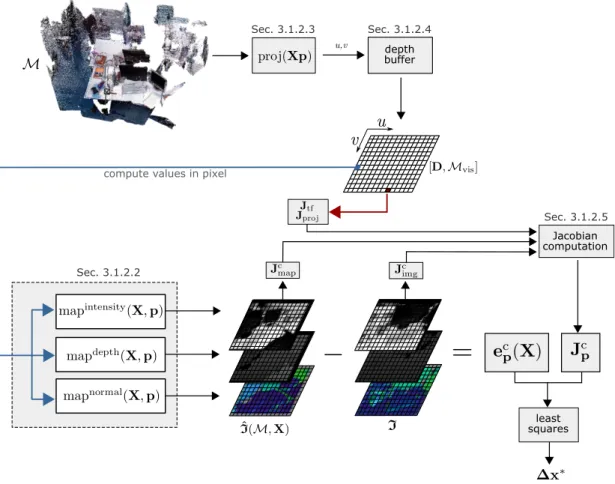
3 Registration and pose estimation 33 3.1 Incremental point cloud matching . . . 343.1.1 Multi-cue photometric point cloud matching . . . 34
3.1.2 Our approach to point cloud registration . . . 37
3.1.2.1 Photometric error minimization . . . 37
3.1.2.2 Cue mapping functions . . . 40
3.1.2.3 Projection models . . . 41
3.1.2.4 Computing visible points using depth buffers . . 42
3.1.2.5 Structure of the Jacobian . . . 43
3.1.2.5.1 Jacobian of transformation . . . 43
3.1.2.5.2 Jacobian of the mapping function . . . 43
3.1.2.5.3 Image Jacobian . . . 44
3.1.2.5.4 Jacobian of the projection function . . . 45
3.1.2.6 Hierarchical approach to photometric minimization 45 3.1.3 Experimental evaluation . . . 46
3.1.3.1 Registration performance and comparison . . . . 46
3.1.3.2 Runtime . . . 50
3.1.4 Related work . . . 51
3.1.5 Conclusion . . . 52
3.2 Constructing a map of environment . . . 52
4 Navigation in static environments 55 4.1 Traversability analysis . . . 56
4.1.1 Our approach to traversability analysis . . . 57
4.1.1.1 What is traversable for a robot . . . 57
4.1.1.2 Sparse 3D map . . . 58
4.1.1.3 Accounting for the vehicle height . . . 59
4.1.1.4 Efficient step detection . . . 59
4.1.1.5 Robust slope detection . . . 60
4.1.1.6 Traversability map estimation . . . 61
4.1.2 Learning traversability directly . . . 62
4.1.3 Experiments . . . 63
4.1.3.1 Timing experiments . . . 63
4.1.3.2 Ground truth comparison . . . 64
4.1.3.3 Traversability estimates obtained in different scenes 66 4.1.3.4 Limitations . . . 68
4.1.4 Related work . . . 68
4.1.5 Conclusion . . . 69
4.2 Exploration . . . 70
4.2.1 Frontier-based exploration . . . 71
4.2.2 Robust exploration using background knowledge . . . 74
4.2.2.1 Utility function for information-driven exploration 75 4.2.3 Predictive exploration . . . 76
4.2.3.1 Querying for similar environment structures . . . 76
4.2.3.2 Loop closures prediction . . . 77
4.2.3.3 Estimating the probability of closing a loop . . . 78
4.2.4 Predictive exploration experiments . . . 79
4.2.4.1 Map comparisons . . . 79
4.2.4.2 Exploration path length . . . 80
4.2.5 Related work . . . 81
4.2.6 Conclusion . . . 82
4.3 Robust homing . . . 83
4.3.1 Robust homing using map consistency checks . . . 84
4.3.1.1 Pairwise inconsistency measure . . . 84
4.3.1.2 Hypothesis test for pairs of scans . . . 86
4.3.1.3 One-vs-all consistency test for scans . . . 87
4.3.2 Adapting consistency check to RGBD data . . . 87
4.3.3 Map consistency estimate for the way to home . . . 88
4.3.4 Homing by rewinding the trajectory . . . 90
4.3.5 Scalability . . . 91
4.3.6 Experiments . . . 91
4.3.7 Related work . . . 98
4.3.8 Conclusion . . . 99
II
Towards dynamic environments
101
5 Detecting motion 103 5.1 Ground estimation and scene clustering . . . 1045.1.1 Range image based ground removal . . . 106
5.1.2 Fast and effective segmentation on laser range data . . . . 110
5.1.3 Experimental evaluation . . . 114
5.1.3.1 Runtime . . . 114
5.1.3.2 Segmentation results . . . 116
5.1.4 Related work . . . 120
5.1.5 Conclusion . . . 122
CONTENTS
5.2.1 Evaluating the alignment quality . . . 124
5.2.2 Experimental evaluation . . . 127
5.2.2.1 Alignment quality . . . 128
5.2.2.2 Runtime . . . 128
5.2.2.3 Support for tracking dynamic objects . . . 129
5.2.2.4 Support for clustering objects . . . 129
5.2.3 Related work . . . 133
5.2.4 Conclusion . . . 135
6 Conclusion 137 6.1 Short summary of key contributions . . . 138
6.2 Contributions to the ROVINA project . . . 140
6.3 Open source contributions . . . 141
1.1 Robots targeted in this thesis. . . 2
2.1 Microsoft Kinect and Asus Xtion sensors. . . 16
2.2 Data from a Microsoft Kinect sensor. . . 16
2.3 LiDARs used in this thesis. . . 17
2.4 LiDAR range image example. . . 17
2.5 Integral image illustration. . . 20
2.6 An example occupancy grid map. . . 21
2.7 Four-neighborhood and eight-neighborhood on a grid. . . 24
2.8 Performance comparison between Dijkstra’s and A* algorithms. . 28
2.9 Coordinate system used in the thesis . . . 29
3.1 Illustration of our approach to multi-cue point cloud registration. 35 3.2 Key ingredients of our framework. . . 38
3.3 S. Gennaro catacombs, recorded with a RobotEye 3D LiDAR. . . 48
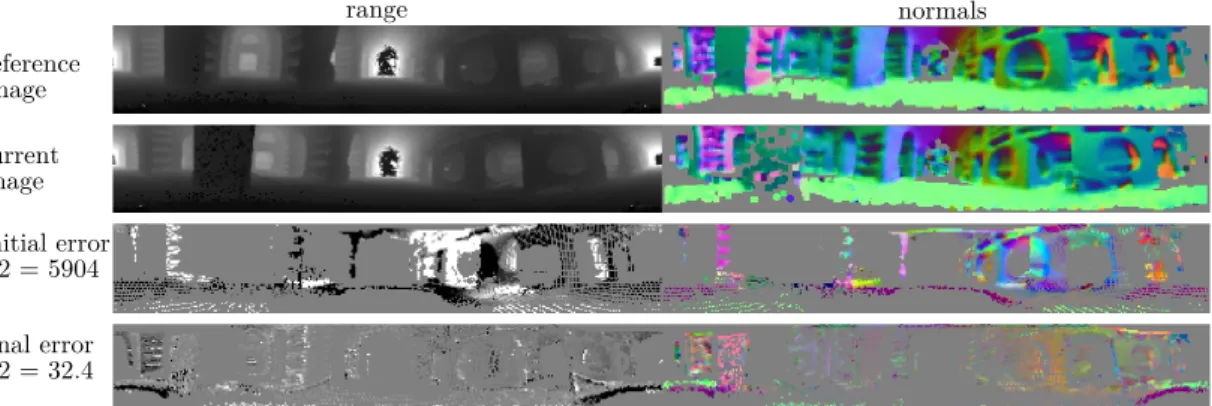
3.4 Error reduction while registering two LiDAR scans. . . 48
3.5 Error before and after registering two LiDAR scans. . . 49
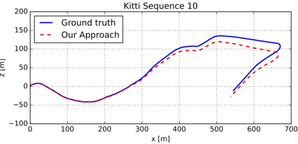
3.6 Ground truth comparison for sequence 10 of the KITTI dataset. . 49
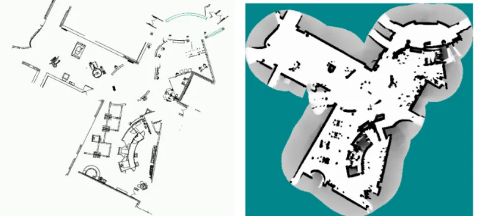
3.7 Part of the catacombs reconstructed by incremental matching. . . 52
3.8 A 3D map of the Roman catacombs viewed from above. . . 54
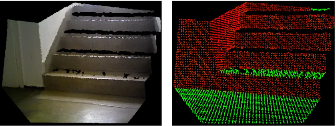
4.1 Traversability of a stair case observed with an RGBD sensor. . . . 56
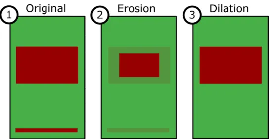
4.2 Erosion-dilation filter. . . 61
4.3 Illustration of traversability prediction from a depth image. . . 62
4.4 Test objects used for evaluating traversability. . . 64
4.5 Ground truth traversability comparison with objects from Figure 4.4. 65 4.6 Robot driving in the Priscilla catacombs. . . 66
4.7 Traversability map of the catacombs. . . 66
4.8 Real-world staircase traversability example. . . 67
4.9 Real-world niche traversability example. . . 67
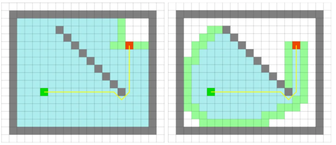
4.10 Real-world outdoor scene traversability example. . . 67 4.11 Robot making decisions on where to go and how to return home. 70
LIST OF FIGURES
4.12 A sequence of images illustrating frontier-based exploration. . . . 73
4.13 Example of the submap retrieval using FabMAP2. . . 76
4.14 Illustration of the loop closures prediction. . . 77
4.15 Illustration of exploration with active loop closing. . . 78
4.16 Predictive exploration outperforming frontier-based one. . . 79
4.17 Distances travelled for the frontier-based and proposed approaches. 80 4.18 Example that depicts pair-wise occlusions of two laser scans. . . . 85
4.19 Example point cloud from the double Asus Xtion system. . . 88
4.20 Map inconsistencies and which paths they influence. . . 89
4.21 Rewinding a trajectory through the office environment. . . 94
4.22 Three rewinded trajectories in different settings. . . 95
4.23 Rewinding a trajectory in a man-made cave in Niederzissen. . . . 96
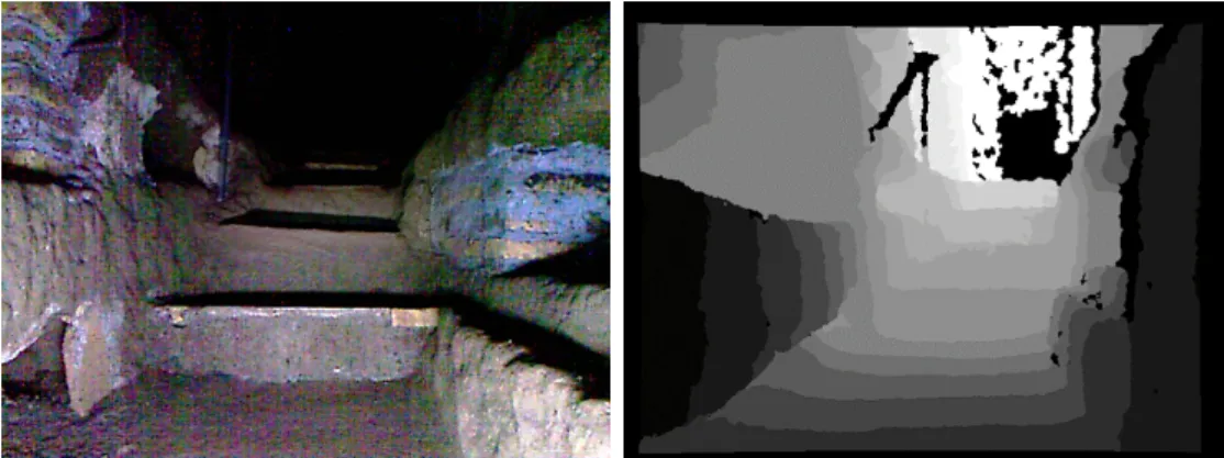
4.24 Rewinding another trajectory in the same setup as in Figure 4.23. 97 5.1 Motivation picture for our segmentation method. . . 105
5.2 Angles generated from range readings that we use to detect ground.107 5.3 Example scene taken with a 64-beam LiDAR. . . 109
5.4 Illustration of our point cloud clustering method. . . 110
5.5 Intuition behind our angle-based separation criterion. . . 111
5.6 Timings for ground removal and clustering on the KITTI dataset. 115 5.7 Timing comparison of Euclidean clustering to our method. . . 115
5.8 Performance comparison of our algorithm to baseline methods. . . 116
5.9 Our clustering compared to grid-based method on 64-beam data. 117 5.10 An example segmentation of a group of people from KITTI dataset.118 5.11 Our clustering compared to the grid-based method on 16-beam data.119 5.12 Motivation analyzing the quality of point cloud matches. . . 124
5.13 Projection with free space. . . 125
5.14 Real and virtual projected images. . . 125
5.15 Example matches of clouds of cars and pedestrians. . . 127
5.16 Changes in the similarity measure with different displacements. . 128
5.17 Our method supporting tracking of a moving object. . . 130
5.18 Using our measure to separate objects with spectral clustering. . . 131
5.19 Examples of hard-to-match vans from KITTI dataset. . . 132
3.1 Relative Pose Error on TUM desk sequences. . . 47
3.2 Average image processing runtime with std. deviation. . . 50
4.1 Timings for normal computation and traversability analysis. . . . 64
5.1 Average runtime and standard deviation per 360◦ laser scan. . . . 115
5.2 Runtime for objects match quality evaluation. . . 129
List of Algorithms
1 Breadth-First Graph Traversal . . . 252 Dijkstra’s Graph Traversal . . . 27
3 Ground labeling . . . 110
Introduction
1.1 General software for robot operation
T
hereare many tasks that are mundane, repetitive, or dangerous that humans do on a regular basis. Typical examples of such tasks range from surveying a particular potentially dangerous area to delivering goods and people. Mobile robots have the potential to aid or even substitute humans in these tasks. In order to carry out such tasks, the robots have to solve a number of challenges such as dealing with complex surroundings, performing mapping, localization, and navigation in static and dynamic environ-ments.Diverse environments put tight constraints on the methods and sensors that can be used by the robots. For example, while a robot that navigates in an urban environment can rely on RGB cameras for detecting objects around it, these cameras have less value in an underground site where there is no light apart from the one that the robot carries itself. To circumvent this problem, sensors like Microsoft Kinect or Asus Xtion can be used as they provide 3D data in the absence of light. However, using these sensors in an outdoor environment is complicated as they provide much less information when their infrared emitter is overwhelmed by the light from the sun. Because of these and other similar constraints, the robots are usually designed with a particular environment in mind and rely on different sensors.
Having different sensors onboard leads to additional complexity in designing the software that can work with the data coming from these sensors. A typical approach is to design custom algorithms that make use of specific sensors. This, however, leads to low code reusability forcing the methods to be reimplemented for every new robot configuration. To avoid these issues, it might be beneficial to invest more time into the design of the software to make it more sensor agnostic, i.e., making the same software work well with multiple types of sensors.
1.2. FOCUS ON ROBOTS OPERATING IN REAL WORLD
Figure 1.1: Robots targeted in this thesis. Left: ROVINA robot in the Roman catacombs of Priscilla.Middle: Clearpath Robotics Husky robot with custom sensor setup at Bonn University campus. Right AnnieWAY self driving car, image courtesy of [43].
In addition to the challenges presented above, robots navigating in real-world environments must make precise estimations about the surrounding world fast. Furthermore, these computations must be performed on an onboard processing unit, and as the amount of power the robot can carry with it is limited, expen-sive computations drain it quickly. The robots, thus, face a complex trade-off between how many computations they must make to understand the surround-ings, build a map, and localize themselves in it, how much they must move to gather new knowledge about the environment, and how much power these ac-tions take. Therefore, one of the cornerstones of developing robust algorithms for robots operating in the real world is efficiency. Robots require information at framerate or even faster and, at the same time, the quality of this information cannot be compromised, as any mistake potentially has a high cost.
In this thesis, we focus on developing robust and efficient algorithms that aid different parts of the robot operation pipeline. We present contributions to mapping, perception and navigation stacks of a robot navigating in real-world environments. The data that we work with come from various sensors, and we are able to process it at framerate on a mobile robot platform. All the methods presented in this thesis have been published at peer-reviewed international con-ferences and journals, and some of them have been made available as open source software.
This thesis is organized as follows. In Part I, we focus on the challenges associated with navigating in static environments, and present our solutions to typical problems that arise in these environments like incremental pose matching, traversability analysis, dealing with broken maps and navigation with or without a valid map. In Part II, we show how these methods can be adapted and extended to work in the environments with dynamic objects.
1.2 Focus on robots operating in real world
Our work is partially motivated by a project for autonomous exploration and dig-ital preservation of hard-to-access archaeological sites such as catacombs. Cata-combs are old Roman burying places used between the 2nd and 5th century in Italy. Even today, they are partially unexplored due to the high risk of entering them. First, most sites are unstable and can collapse. Second, most of the (non-ventilated) catacombs yield a high concentration of radioactive radon gas so that humans are only allowed to stay in these sites for 15 min-30 min to prevent serious health issues. Thus, robots are an excellent tool for the exploration, mapping, and digital preservation of such sites. To achieve that, the robots have to operate and explore the space in a completely autonomous fashion. As part of a joint effort in the ROVINA project, we have developed a robot depicted on the left of Figure 1.1, that is able to navigate and map catacombs of Priscilla in Rome.
Even though catacombs are challenging environments, they have one trait that simplifies robot operation: they are static. The static assumption holds for most underground environments but rarely for urban ones. Therefore, we have implemented a number of extensions to the methods required for static environ-ment navigation to aid the robot in dealing with the changing environenviron-ments. The presence of dynamic obstacles in an environment has a significant impact on the reasoning behind the actions of the robot. When targeting dynamic environ-ments, we target mobile robots such as one depicted in the middle of Figure 1.1, navigating the campus at the University of Bonn, as well as robots tailored for autonomous driving, such as the AnnieWAY car from the University of Karlsruhe shown on the right of Figure 1.1.
We focus on designing algorithms that work at least at the frame rate of the sensors mounted on real robots with constrained computational power while being generic and applicable to different indoor and outdoor environments. While a single Ph.D. thesis is, probably, not enough to completely solve perception, mapping, localization, and navigation of mobile robots in static and dynamic environments, we focus on providing the implementations for a number of crucial parts of these tasks. The contributions of this thesis are solutions to different aspects of the robot perception and navigation tasks that use a depth sensor as the source of information about the surrounding world. Depth sensors have been popularized by the introduction of the Microsoft Kinect sensor in 2010 and the consequent introduction of the Asus Xtion in 2011, as well as the Velodyne PUCK LiDAR in 2014. These sensors made it possible to obtain 3D information about the environment on a cheap mobile robot. We treat the data coming from Microsoft Kinect, Asus Xtion and LiDARs uniformly and represent it in the form of range images, as this representation allows for efficient processing of the sensor data. For more information on range images, we refer the reader to Section 2.2.
1.2. FOCUS ON ROBOTS OPERATING IN REAL WORLD
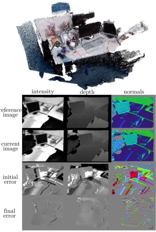
We envision that a robot that carries various sensors such as Microsoft Kinect, Asus Xtion or a LiDAR navigating an environment autonomously, must address a number of challenges in order to carry out its mission safely. We assume that the robot starts without any knowledge about the environment, and its goal is to explore this environment fully. To do this, the robot must be able to localize itself in an unknown environment. A typical approach to solving this problem is simultaneous localization and mapping (SLAM) as the robot must build its map and localize itself in it. SLAM is a relatively well-studied problem [119] and relies on a number of techniques. In this thesis, we only consider the graph-based variant of SLAM, where all the poses where the robot takes measurements are organized into a pose-graph representation that allows for integrating in-formation from different sensor measurements taken at various positions, and optimizing the resulting graph based on this. We refer the reader to a tutorial by Grisetti et al. [47] for more details on pose-graph construction and typical optimization techniques. Building such a graph usually consists of incrementally matching the point clouds while moving in an environment adding the edges with relative constraints to the graph, detecting so-called loop closure edges to avoid incremental error accumulation and an optimization algorithm that is able to op-timize this graph. In this thesis, we specifically address the point cloud matching by implementing our own generic point cloud matching algorithm, which takes advantage of the information provided by multiple cues available from the sensor data by optimizing the photometric error. To support incremental matching, this component must run at the frame rate of the sensor and work reliably utilizing all available information, such as color, depth and surface normals.
Having a consistent map of the currently observed environment allows the robot to plan paths through it in order to discover more about it. While this is not the main contribution of this thesis, we have also created a method that allows exploring an unknown environment efficiently. However, being able toplana path is not enough to guarantee safe navigation in an unknown environment along this path. The robot must know, which parts of the surrounding environment are traversable and if the map that it has built so far is reliable for navigation. We contribute solutions to both of these challenges. We analyze the traversability of the currently seen environment, and integrate it into a single consistent map while continuously monitoring the consistency of this resulting map. If, at any point in time, a map inconsistency is detected, the robot must be able to recover itself not relying on this inconsistent map. Such a method for robust robot recovery is also one of the main contributions of this thesis.
A robot equipped with the functionality described above is capable to au-tonomously explore a static environment, i.e., the one that does not change with time. This assumption holds for caves, catacombs, warehouses, and some
and-rescue scenarios, but is not valid for outdoor navigation in typical urban scenarios. To account for this, we extend the set of methods described above by further methods for scene analysis to detect objects that might be moving in the scene. In particular, we developed a method that clusters the data observed by the robot into meaningful objects in an unsupervised fashion. These objects can then be tracked with any tracking algorithm to find out if they are dynamic or static. To this end, we also implemented a robust measure that provides the information if two objects match each other using the notion of the shape of the objects. While these contributions do not solve navigation in dynamic en-vironments, we believe they are an important cornerstone to implementing such algorithms.
1.3 Main contributions
This thesis presents novel solutions to several relevant problems in the context of mobile robots operating with depth sensors. It provides contributions to multiple aspects of robot perception and navigation in the real world under computational constraints stemming from the fact that all these algorithms are capable of run-ning on board of a mobile robot platform. This section provides a short summary of the central achievements and methods that contribute to the state of the art in robotics.
The first contribution presented in this work is in the context of point cloud matching. Our method for photometric point cloud matching [26] pushes the state of the art forward by incorporating additional modalities into the standard photometric matching, presented by the dense visual odometry [67] (DVO) ap-proach. Our method allows for matching point clouds originating from various sensors, such as Microsoft Kinect or LiDARs at the frame rate of the used sensor. It builds upon DVO but allows using additional cues to aid the matching pro-cedure. Running it on real-world data shows that we can maintain a very good matching performance under various conditions using different sensors while us-ing the exact same code base, which we have also made available as an open source library. The method is presented in-depth in Section 3.1.
The second contribution of this thesis targets the scene analysis that can be performed on the range data perceived by the robot at real time. It is a method for performing scene traversability analysis [14]. This information is crucial for a robot when navigating in complex environments. This method has been de-veloped as part of the EC-funded ROVINA project, where we have deployed a robot to explore the Roman catacombs for the tasks of cultural heritage preser-vation. The method analyzes if the surroundings are traversable by the robot, which is the prerequisite for collision-free, autonomous navigation. The method
1.3. MAIN CONTRIBUTIONS
is strictly geometrical, running at the frame rate of the sensor on computationally constrained hardware using input data from cheap and rather noisy sensors. The software developed for this method has formed the basis for navigation in real underground sites in Rome and has been used by multiple components running on the robot such as the navigation and exploration stacks, proving it to be a viable method for analyzing traversability of static environments. This method is presented in-depth in Section 4.1.
The third contribution of this thesis builds upon the same input data and targets the navigation stack of the robot operating in an unknown environment. We have developed systems that allow the robot to navigate the environment autonomously, but the main contribution of this part of this work is a method that focuses on detecting if the map constructed by the robot driving through a static environment is in an inconsistent state, and on handling the safe return of the robot to the starting point by unwinding the recorded odometry trajectory [10, 96]. This method continuously retracts over the odometry data taken on the way up to the place where the mapping system failed, and corrects its position using point cloud matching. The main contribution of this method is not as much in a single state-of-the-art method, but in a combination of the above mentioned methods into a single system that has been successfully used within ROVINA project on a real robot platform in real underground environments. It is presented in Section 4.3 of this thesis.
The fourth contribution of this work is a robust and efficient clustering algo-rithm for point clouds that uses a novel cluster separation criterion defined on range images [11, 13]. The performance of this algorithm is guided by a single bounded threshold value and has performance as good as the classical Euclidean clustering while being orders of magnitude faster. It has been tested on real world data acquired with various Velodyne LiDARs and delivers state-of-the-art performance much faster than the frame rate of the sensor that provides data to it. More details on this method can be found in Section 5.1.
Lastly, our fifth contribution is a method to analyze the quality of the align-ment between the objects clustered with a clustering algorithm in a scenario where the objects have to be tracked [12]. We again make use of the range image data representation and use free space surrounding the objects as an additional criterion for providing a single score for quantifying the quality of a match of pairs of objects. For more details on this method, please refer to Section 5.2.
Overall this thesis presents five contributions, each of which target an im-portant part of the robot mapping, navigation, or scene analysis pipeline. All methods presented here are tested on real-world data and on real robots navigat-ing challengnavigat-ing environments. These methods share the fact that they work on range data and on their range image representation. Most of the contributions
presented here have been published as open source software, either as part of the ROVINA open source software suite or standalone.
1.4 Publications
Parts of this thesis have been published in the following peer-reviewed conference and journal articles:
• I. Bogoslavskyi, O. Vysotska, J. Serafin, G. Grisetti, and C. Stachniss. Ef-ficient traversability analysis for mobile robots using the kinect sensor. In
Proc. of the Europ. Conf. on Mobile Robotics (ECMR), 2013
• I. Bogoslavskyi and C. Stachniss. Fast range image-based segmentation of sparse 3d laser scans for online operation. In Proc. of the IEEE/RSJ Int. Conf. on Intelligent Robots and Systems (IROS), 2016
• I. Bogoslavskyi, M. Mazuran, and C. Stachniss. Robust Homing for Au-tonomous Robots. In Proc. of the IEEE Int. Conf. on Robotics and Au-tomation (ICRA), 2016
• D. Perea-Ström, I. Bogoslavskyi, and C. Stachniss. Robust exploration and homing for autonomous robots. In Journal on Robotics and Autonomous Systems (RAS), volume 90, pages 125–135, 2017
• I. Bogoslavskyi and C. Stachniss. Analyzing the quality of matched 3d point clouds of objects. InProc. of the IEEE/RSJ Int. Conf. on Intelligent Robots and Systems (IROS), 2017
• I. Bogoslavskyi and C. Stachniss. Efficient online segmentation for sparse 3d laser scans. In Photogrammetrie – Fernerkundung – Geoinformation (PFG), volume 85, pages 41–52, 2017
• B. Della Corte*, I. Bogoslavskyi*, C. Stachniss, and G. Grisetti. A general framework for flexible multi-cue photometric point cloud registration. In
Proc. of the IEEE Int. Conf. on Robotics and Automation (ICRA), 2018. * authors have contributed equally
1.5. COLLABORATIONS
1.5 Collaborations
Some work included in the publications presented above has been done in collab-oration with other people. The work “Efficient Traversability Analysis for Mobile Robots using the Kinect Sensor” [14] has been carried out at the University of Freiburg along with Olga Vysotska and Jacopo Serafin under the supervision of Giorgio Grisetti and Cyrill Stachniss. Olga has been helping in implementing the traversability algorithm, while Jacopo has provided his help in initial adaptation of the algorithm to the robot platform that was in the initial stage of development in Rome at the time.
The work “Robust Homing for Autonomous Robots” [10] has been carried out in collaboration with Mladen Mazuran. Mladen has provided his advice on adapting the method from his earlier work [80] to a new sensor.
We further collaborated with Daniel Perea-Ström on the paper “Robust ex-ploration and homing for autonomous robots” [96]. This paper focuses on imple-menting a robust and fail-safe system for robot exploration that is able not only to use the geometry of the environment to explore the environment efficiently, but is also able to detect when the underlying map of the environment is broken and in this case returns the robot safely to the initial position. In this work, Daniel was mostly focusing on exploration, while my focus has been the robust homing and integration of the components into a single system.
Finally, our last collaboration has been carried out along with Bartolomeo Della Corte, who is a student at the lab of Giorgio Grisetti. Bartolomeo and I have put equal efforts into developing the proposed algorithm and therefore share the first authorship of the paper.
Basic techniques
2.1 Least Squares
M
ultiple problems in robotics can be addressed by local minimiza-tion of squared errors. This type of minimizaminimiza-tion problems maps directly to the least squares formulation. The idea behind the least squares method is that if we can define a function that con-sists of a sum of squares of values that we have some control over, we can use efficient iterative techniques to find such a configuration that minimizes the re-sulting sum. It is used in many robotics applications, e.g., using iterative closest point algorithms for point cloud registration or in various graph optimization techniques for simultaneous localization and mapping. In this section we will outline the general least squares formulation and method as well as the typi-cal assumptions made in order to solve the underlying non-linear least squares problems efficiently.2.1.1 Least squares formulation
Let x = [x1, x2, . . .]⊤ ∈ IRn be a vector of values xi. Then we can talk about
minimizing the function F(x) that is defined as a sum of squares of functions fi
applied to x: F(x) = 1 2 m ∑ i=1 (fi(x))2, (2.1)
where fi : IRn → IR, i = 1, . . . , m are given functions, and m ≥ n. We want to
find a local minimizer x∗ for the functionF(x):
x∗ =argmin
x
2.1. LEAST SQUARES
We assume that the cost function F is differentiable and so smooth that the following Taylor expansion holds:
F(x+h) = F(x) +h⊤g+ 1 2h
⊤Hh+O(∥h∥3
), (2.3)
whereg is the gradient:
g ≡F′(x) = ∂F ∂x1(x) . . . ∂F ∂xn(x) , (2.4)
and His the Hessian:
H≡F′′(x) = [ ∂2F ∂xi∂xj(x) ] . (2.5)
2.1.2 Necessary and sufficient conditions for a local
mini-mizer
Ifx∗ is a local minimizer, then:
g∗ ≡F′(x∗) = 0. (2.6)
This condition is a necessary condition, but not a sufficient one, as such a solution can also be a saddle point, i.e., a point which is a local minimum in one direction and a local maximum in another direction. To determine if a given stationary pointxs is a local minimizer we can use the second order term in the
Taylor series: F(xs+h) =F(xs) + 1 2h ⊤H sh+O(∥h∥ 3 ), (2.7)
where Hs = F′′(xs). From the fact that F(xs+h) must be bigger than F(xs)
for any h we can formulate a sufficient condition for a local minimizer: if xs is a
stationary point andF′′(xs)is positive definite then xs is a local minimizer.
2.1.3
Descent methods
It is usually impossible to find the minimum ofF(x) directly, therefore a variety of iterative methods are used in order to descent into the minimum. We can search for the solution x∗ by iteratively moving in the direction towards a local minimizer. The direction towards the local minimizer has to be determined at each iteration. Roughly speaking, we can describe the procedure as one consisting of the following steps:
1. Search for the direction of descent h.
2. Make a step of some size αh in that direction.
3. Repeat the procedure until convergence.
By making a step we mean evaluating the function F for the argument x+αh. From the Taylor expansion in Equation (2.3):
F(x+αh) ≃ F(x) +αh⊤F′(x). (2.8) We say, that h is a descent direction if F(x+αh) is a decreasing function of α
atα = 0.
2.1.3.1 Steepest descent
When performing the optimization procedure we can pick bothh andα. Usually we want to minimize the number of steps we need to make in order to reach the minimum of the function F(x). We can say that we perform a stepαh, where α
is positive. Then, using Equation (2.8), we can write the relative gain in function value: lim α→0 F(x)−F(x+αh) α∥h∥ = αlim→0 F(x)−(F(x) +αh⊤F′(x)) α∥h∥ = lim α→0 −αh⊤F′(x) α∥h∥ = − 1 ∥h∥h ⊤F′(x) dot product = − ∥F′(x)∥cosθ, (2.9) where, θ is an angle between h and F′(x). Therefore, we see that the biggest change in function is reached if θ = π, i.e., h = −F′(x). This choice of α and
h is called “steepest descent” but it comes at a cost. The final convergence of this method is slow as the derivative F′(x) approaches zero at the final stages of the optimization. To mitigate this behavior other methods, like the Newton’s method, are commonly used.
2.1.3.2 Newton’s method
To have good convergence in the final stage we must pick the steph better than when using the steepest descent method. We can derive the Newton’s method from the fact that x∗ is a stationary point, i.e., F′(x∗) = 0. This is a non-linear system of equation. To solve it we consider its Taylor expansion:
F′(x+h) = F′(x) +F′′(x)h+O(∥h∥2
) ≃ F′(x) +F′′(x)h
= F′(x) +Hh. (2.10) Setting the termF′(x+h) to zero following the logic described above we search for the best direction vectorh as a solution to
2.1. LEAST SQUARES
Solving this equation allows us to find the current best direction vector h and iterate by
x→x+h. (2.12)
2.1.4 Non-linear least squares
In the case when the functionsfiare non-linear, more efficient methods are usually
used in order to find the minimum of F(x). These methods avoid computing the second derivatives of function F(x). More formally, we want to find x∗ =
argminxF(x), where F(x) = 1 2 m ∑ i=1 (fi(x))2 = 1 2f(x) ⊤f(x). (2.13)
Provided, thatfhas continuous second partial derivatives, we can write its Taylor expansion:
f(x+h) =f(x) +J(x)h+O(∥h∥2
), (2.14)
whereJ is the Jacobian. Making use of Equation (2.1), the partial derivatives of
F are: ∂F ∂xj (x) = ∂( 1 2 ∑m i=1(fi(x)) 2) ∂xj = m ∑ i=1 fi(x) ∂fi ∂xj (x). (2.15)
Thus the gradient is
F′(x) = J(x)⊤f(x). (2.16) Following the same logic, we can also estimate the Hessian:
F′′(x) = J(x)⊤J(x) +
m
∑
i=1
fi(x)fi′′(x). (2.17)
Such Hessian can be complicated to compute as it involves the second derivatives of functionsfi. In order to avoid computing them, approximations are used that
allow simplifying these equations. The most commonly used method to avoid computing the Hessian is the Gauss-Newton method presented in the section below.
2.1.4.1 Gauss-Newton method
The Gauss-Newton method approximates the functions f by linearizing f in the neighborhood of x, i.e., for small ∥h∥, the Taylor expansion of f is:
f(x+h)≃l(h)≡f(x) +J(x)h=f+Jh. (2.18) 12
The same operation can be applied to the sum of all functions f, i.e, to the F function: F(x+h)≃L(h) ≡ 1 2l(h) ⊤l(h) = 1 2f ⊤f+h⊤J⊤f+1 2h ⊤J⊤Jh = F(x) +h⊤J⊤f+1 2h ⊤J⊤Jh. (2.19)
From this it is easy to derive that the gradient and the Hessian of Lare:
L′(h) = J⊤f+J⊤Jh (2.20)
L′′(h) = J⊤J. (2.21)
Now we can find a unique minimizer by solving for h:
(J⊤J)h=−J⊤f. (2.22) And the typical next step is then: x → x+αh. The classical Gauss-Newton method uses α= 1.
2.1.4.2 Levenberg-Marquardt method
Levenberg and Marquardt suggested to use a damped Gauss-Newton method, where the step h is defined by solving the damped version of Equation (2.22):
(J⊤J+αI)h =−J⊤f, (2.23) where Iis an identity matrix.
For allα >0the coefficient matrix is positive definite which ensures that the steph, picked in such a way, is always taken towards the descent direction, which is not the case for Gauss-Newton algorithm, e.g., in the case of “overshooting” the correct solution. For large values of α the step is inverse proportional to
α itself and is oriented in the steepest descent direction. This is good if the current iteration is far from the local optimum. If, however, α is very small the method converges to a standard Gauss-Newton method, which ensures good final convergence. Usually it is a good idea to start with larger values of α related to the Jacobian:
αo =τ·max i {a
(0)
ii }, (2.24)
wherea(0)ii are the elements of matrix A0 =J(x0)⊤J(x0), andτ is the parameter
chosen by the user. The values ofα can be reduced with iterations depending on the gain ratio
ϱ= F(x)−F(x+h)
2.1. LEAST SQUARES
This way, at the start of the minimization, we use the steepest gradient de-scent, and towards the end of the minimization procedure we switch to the Gauss-Newton method. Overall, using Levenberg-Marquardt algorithm in place of Gauss-Newton method results in a more robust solution less sensitive to a bad initial guess.
2.1.5 Use cases in robotics
Non-linear least-squares techniques have multiple typical use cases in robotics. In this thesis they are used for point cloud registration and pose graph optimiza-tion. Most of the time the observations are correlated and we need to extend the formulation to account for this and the measurement uncertainty. In this case, functions fi(x) represent errors between the estimated constraint and the
measured one. We will denote these errors as
ei(x, zi) =hi(x)−zi, (2.26)
where, hi(x) is a function that maps x to a predicted measurement, while zi is
the actual observation.
If the additional information on the reliability of these measurements is avail-able, we can incorporate it into the squared error terms. We can therefore rewrite Equation (2.13) for the error term defined in Equation (2.26) in a matrix form as
E(x,z) = 1
2e(x,z)
⊤Λ e(x,z), (2.27)
whereΛ is the so-called information matrix. In this thesis, we assume our mea-surements to be uncorrelated so the information matrix only has diagonal values that depict our certainty in a particular sensor. This matrix propagates naturally through all the equations presented above, resulting in Equation (2.22) to have the form
(J⊤Λ J)h=−J⊤Λ e(x,z). (2.28)
2.1.6
Relation to adjustment theory
The least-squares formulation presented above, maps to well-known adjustment models [38, 88]. In this theory we have a vector of observations L, a vector of initial valuesX0 and a vector of adjustments ˆx. Combining these vectors yields
a vector of balanced parameters Xˆ: ˆ
X=X0+ ˆx. (2.29)
We can further define a vector of the observation estimates L0 that depends on
the current state X0 and some observation function
L0 =f(X0), (2.30)
which leads to the observations to be formally defined as
L=L0
+l, (2.31)
where,l is the shortened observation vector
l=L−L0. (2.32)
It is common to think of a vectorv as a vector of improvements that, combined with the shortened observation vector l, allows to define a functional model in the following matrix form:
l+v=Axˆ, (2.33) where A is the matrix of partial derivatives that maps to the Jacobian J in the previous sections. The goal of our optimization procedure is to minimize the needed improvementsvby minimizing the expressionv⊤v, from Equation (2.33). This results in the final equation
A⊤Axˆ =A⊤l, (2.34)
that we can solve with respect toxˆ to minimize the needed improvements. To account for the uncertainty of the measurements, we use the Gauss-Markov model. The covariance matrixΣll of this model is defined through a variance σ2o
that represents an absolute precision with which we can measure a particular modality, and the cofactor matrixQll, such that
Σll =σo2Qll. (2.35)
Here, the inverse of the cofactor matrix corresponds to the information matrix presented in the previous sections
Q−1
ll =Λ. (2.36)
In adjustment models, this matrix is usually called the weighting matrixPof the observations vector. This matrix consists of diagonal elements, each of which is a variance of a particular modality σ2
o/σi2 and can be homogenized as
Λ =P=P12P
1
2. (2.37)
Multiplying the Equation (2.33) by the matrixP12 from both sides, and
minimiz-ing the value of v⊤vusing the resulting equation, allows us to rewrite the Equa-tion (2.34) in the following form:
A⊤PAxˆ =A⊤Pl, (2.38)
which directly maps onto Equation (2.28). Therefore, without the loss of gener-ality, we can follow the notation presented in Section 2.1.4 in the remainder of this thesis for all problems that require a least-squares solution.
2.2. DEPTH AND RANGE IMAGES
Figure 2.1: Left: Microsoft Kinect (image courtesy of Microsoft), Right: Asus Xtion (image courtesy of Asus)
2.2
Depth and range images
In our work we heavily rely on range images. These images can be obtained in two ways. They can be provided by a sensor directly or can be generated as a projection of a 3D point cloud. There is also a way to generate a depth image from a stereo RGB image pair but this is not considered in this thesis.
2.2.1 Sensors that produce range data
Typical sensors that provide a range image out of the box are Microsoft Kinect and Asus Xtion as shown in Figure 2.1. These sensors generate depth data by emitting an infrared pattern and perceiving the distortion of this pattern.
Example images that are produced by such sensors can be seen in Figure 2.2. Every pixel of a range image contains a distance to the object in the real world. Because the image has rigid pixel structure and a depth value for each pixel, it allows to reconstruct 3D representation of the environment measured by the sensor.
A slightly less common case is to reconstruct a range image from a 3D scene or from a LiDAR sensor. A spherical or a cylindrical projection can be used in order to project the 3D points onto an image plane to generate a (virtual) range image. In this thesis, we use Velodyne and Ocular LiDARs shown in Figure 2.3. The main method for generating a range image from these LiDARs is to fix the angular resolution of the horizontal and the vertical viewport, thus mapping
Figure 2.2: Data from a Microsoft Kinect sensor. Left: RGB,Right: Depth
Figure 2.3: Left: 16-beam Velodyne PUCK LiDAR (image courtesy of Velodyne), Middle:
64-beam Velodyne HDL-64E LiDAR (image courtesy of Velodyne) Right: Ocular Robotics RobotEye RE05 3D LiDAR (image courtesy of Ocular Robotics).
range readings to discrete pixels of a range image. Using the angular resolution of the laser beams provided by the sensor manufacturer, we can minimize beam overlapping, thus generating a nearly perfect mapping from beams to a range image.
This results in images that look as presented in Figure 2.4. Note, that the range images generated from a Velodyne sensor span full view of 360 degrees around the sensor and wrap on the border, i.e., an object on the right border of an image can also appear on the left of the image. In this particular example the wall that goes out of the image on the left continues on the right.
Figure 2.4: Top: 3D representation of a single LiDAR scan,Bottom: range image constructed from the same data. The part of the image that corresponds to the floor is removed for clarity.
2.2. DEPTH AND RANGE IMAGES
2.2.2
Efficient data representation
Range images are useful to perform efficient computations on 3D data. Note, that usually range images are considered to be 2.5D data representation, as the 3D points that fall into the same pixel under a projection operation, have to be discretized into the pixel coordinates, and each pixel has a single range value stored in it. However, in the case of Velodyne LiDARs, we can guarantee that the range image contains all data from the 3D scene as we have control over how these data are generated. The Velodyne sensor rotates a vertical array of 16, 32, 64 or 128 beams to produce the full spherical scene representation. The angular resolution of the placement of the beams and the speed of rotation are given as parameters of the sensor, thus, we can tailor the size of the range image to match the number of beams up to a negligible error in the laser firing timings.
Range images are a useful representation of the 3D data as they allow for an extremely efficient neighbor search with O(1) complexity. We are making use of this property in multiple parts of this thesis. First, we propose a generalized framework for photometric matching of point clouds. The proposed method runs at the frame rate of the sensor partially due to the fact that we can avoid searching for neighbors of each point in 3D, which is a typical step in point cloud registration methods. This simplification is only possible because we are using the image representation of the 3D data. Additionally we make use of range images in the clustering section of this thesis, where we process the data received from a Velodyne sensor to find clusters of objects of interest in the vicinity of the robot. We achieve performance comparable to a standard Euclidean clustering while having the runtime performance orders of magnitude faster. This speed up comes from the fact that we analyze the neighbors of a point on a grid defined by the range image. As the neighbor search runs in constant time, it allows us to process all data coming from the sensor at up to 667 Hz. Lastly, we extend our clustering method by adding a fast quality assessment method to detect if the clouds of two objects match. We also make extensive use of range images in this part of this work. Range image representation is again responsible for quick execution of our algorithm on data from a real world dataset, and for quick estimation of the free space around the object.
2.2.3
Fast normal computation
Range image representation allows for fast and effective normal direction com-putation. Classically, to compute a normal vector of a point, a plane is fitted to the 3D points within some neighborhood of the query point. The normal is then computed as a direction of the normal vector to this plane. This mathematically sound approach, however, comes at a cost as it requires searching for neighbors for
every point. This algorithm, at best, has an asymptotic complexity ofO(nlogn), where n is the number of the points in the whole point cloud. When working on 3D data and the number of points is high, the runtime of algorithms that rely on searching for neighbors in 3D is doomed to deteriorate. As the mobile robots are usually computationally constrained, it is a desirable feature to avoid the potentially costly operations.
The range image representation outlined in the previous section is strictly structured as opposed to the unordered 3D point cloud representation. The points that lie close in the real world get projected to the nearby pixels in the range image representation. This allows us to perform the neighbor search in the image plane. Because the image has a rigid grid structure, neighborhood search has the complexity of O(1) which has a desirable property of being independent from the number of points in the point cloud.
Our approaches exploit information about the surface normals of the perceived environment. Thus, the first operation we perform is to compute a normal vector for each 3D point using the depth image. For a point p, we can compute its normal by considering a Gaussian distribution with parametersµ and Σ, which models the distribution of the neighboring points of p. The eigenvector of Σ, which corresponds to the smallest of the three eigenvalues, provides the direction of the normal.
We apply a fast method for normal extraction that exploits the structure of the input similar to Holzeret al.[61], and take advantage of the underlying hardware. We can rewrite the computation of the mean and the covariance matrix as:
µ = 1 N ∑ i pi | {z } P = 1 NP (2.39) Σ = 1 N ∑ i pipi⊤ | {z } S −µµ⊤ = 1 NS−µµ ⊤, (2.40)
where N is the number of neighbors of the point p. If we know the terms P
and S, we can compute the covariance matrix and thus the normals in constant time. By exploiting the fact that we are using a depth image as the input, we can realize the computation of P and S in constant time too through the use of integral images.
The integral imageI(i, j)→(Pij,Sij)maps the pixel coordinates(i, j)to the
tuple (Pij,Sij) such that
Pij = i ∑ k=1 j ∑ l=1 pkl Sij = i ∑ k=1 j ∑ l=1 pklpkl⊤, (2.41)
2.2. DEPTH AND RANGE IMAGES
Figure 2.5: Left: an image filled with integer pixel values. Right: an integral image computed from the image on the left. The value stored in the pixel labeledAon the right is the sum of all pixels in a red rectangle on the left. The sum of all elements in a blue rectangle from the original image is computed by the provided formula.
where pkl corresponds to the 3D point, which is observed by the pixel (k, l).
Thus, this integral image is a 2D array where the position(i, j)contains the sum
Pij and the squared sum Sij of all other points visible in the rectangular area
between (1,1) and (i, j). Exploiting the fact that the terms S and P support addition and subtraction, we can determine S and P for any rectangular region
(i1, j1)to (i2, j2) in the integral image by
I(i1, j1, i2, j2) =I(i2, j2) +I(i1, j1)− I(i1, j2)− I(i2, j1). (2.42)
By processing the depth image from the top left to the lower right corner, each computation exploits the result of the previous step leading to a constant time computation of Pij and Sij for each pixel. Figure 2.5 depicts an integral image
computed from a toy example image filled with integer values.
Note that the computation of the normals through the integral image is an approximation. The reason is that only rectangular image regions can be queried with Equation (2.42) and the queries are performed in image coordinates and not in world coordinates. The appropriate size of the region, however, can easily be determined given the distance of the query point to the camera.
The implementation of the algorithm described above can furthermore exploit the SSE extensions of Intel CPUs by operating on packed structures of four floats. The points are stored as homogeneous vectors p= [x y z 1]⊤. The terms P and
Sare stored as a 4-dimensional vector and as a4×4matrix respectively. Adding points to an accumulator P using this representation, results in a homogeneous component that contains the number of points. This has the effect of removing conditional instructions and of performing the evaluation almost entirely in the SSE subsystem of the CPU. This provides a speed up of a factor of 3 compared to an implementation of the same algorithm without SSE instructions.