UC Berkeley
UC Berkeley Previously Published Works
Title
Dominant currency paradigm†
Permalink
https://escholarship.org/uc/item/52b56456
Journal
American Economic Review, 110(3)
ISSN 0002-8282 Authors Gopinath, G Boz, E Casas, C et al. Publication Date 2020-03-01 DOI 10.1257/aer.20171201 Peer reviewed
Dominant Currency Paradigm
∗
Gita Gopinath
Emine Boz
Camila Casas
Harvard IMF Banco de la Rep ´ublica
Federico J. D´
ıez
Pierre-Olivier Gourinchas
Mikkel Plagborg-Møller
IMF UC Berkeley Princeton
June 25, 2019
Abstract
We propose a ‘dominant currency paradigm’ with three key features: dominant cur-rency pricing, pricing complementarities, and imported inputs in production. We test this paradigm using a new data set of bilateral price and volume indices for more than 2,500 country pairs that covers 91% of world trade, as well as detailed firm-product-country data for Colombian exports and imports. In strong support of the paradigm we find that: (1) Non-commodities terms of trade are uncorrelated with exchange rates. (2) The dollar ex-change rate quantitatively dominates the bilateral exex-change rate in price pass-through and trade elasticity regressions, and this effect is increasing in the share of imports invoiced in dollars. (3) U.S. import volumes are significantly less sensitive to bilateral exchange rates, compared to other countries’ imports. (4) A 1% U.S. dollar appreciation against all other currencies predicts a 0.6% decline within a year in the volume of total trade between coun-tries in the rest of the world, controlling for the global business cycle. We characterize the transmission of, and spillovers from, monetary policy shocks in this environment.
∗
This paper combines two papers:Casas et al.(2016) andBoz et al.(2017). We thank Isaiah Andrews, Richard Baldwin, Gary Chamberlain, Michael Devereux, Charles Engel, Christopher Erceg, Doireann Fitzgerald, Jordi Gal´ı, Michal Koles ´ar, Philip Lane, Francis Kramarz, Brent Neiman, Maury Obstfeld, Jonathan Ostry, Ken Rogoff, Arlene Wong, and seminar participants at several venues for useful comments. We thank Omar Barbiero, Vu Chau, Tiago Fl ´orido, Evgenia Pugacheva, Jianlin Wang for excellent research assistance and Enrique Montes and his team at the Banco de la Rep ´ublica for their help with the data. The views expressed in this paper are those of the authors and do not necessarily represent those of the IMF, its Executive Board, or management, nor those of the Banco de la Rep ´ublica or its Board of Directors. Gopinath acknowledges that this material is based on work supported by the NSF under Grant Number #1061954 and #1628874. Any opinions, findings, and conclusions or recommendations expressed in this material are those of the author(s) and do not necessarily reflect the views of the NSF. All remaining errors are our own.
1
Introduction
Nominal exchange rates have always been at the center of fierce economic and political debates on
spillovers, currency wars, and competitiveness. It is easy to understand why: in the presence of price
rigidities, nominal exchange rate fluctuations are associated with fluctuations in relative prices and
therefore have consequences for real variables such as the trade balance, consumption, and output.
The relationship between nominal exchange rate fluctuations and other nominal and real
vari-ables depends critically on the currency in which prices are rigid. The first generation of New
Keyne-sian (NK) models, the leading paradigm in international macroeconomics, assumes prices are sticky
in the currency of the producing country. Under this ‘producer currency pricing’ paradigm (PCP), the
law of one price holds and a nominal depreciation raises the price of imports relative to exports (the
terms-of-trade) thus improving competitiveness. This paradigm was developed in the seminal
con-tributions ofMundell(1963) andFleming(1962),Svensson and van Wijnbergen(1989), andObstfeld
and Rogoff(1995).
There is, however, pervasive evidence that the law of one price fails to hold. Out of this
ob-servation grew a second pricing paradigm. In the original works of Betts and Devereux(2000) and
Devereux and Engel(2003), prices are instead assumed to be sticky in the currency of the destination
market. Under this ‘local currency pricing’ paradigm (LCP), a nominal depreciation lowers the price
of imports relative to exports, a decline in the terms-of-trade, thus worsening competitiveness. Both
paradigms have been extensively studied in the literature and are surveyed inCorsetti et al.(2010).
Recent empirical work on the currency of invoicing of international prices questions the validity
of both approaches. Firstly, there is very little evidence that the best description of pricing in
inter-national markets follows either PCP or LCP. Instead, the vast majority of trade is invoiced in a small
number of ‘dominant currencies,’ with the U.S. dollar playing an outsized role. This is documented in
Goldberg and Tille(2008) and inGopinath(2015). Secondly, exporters price in markets characterized
by strategic complementarities in pricing that give rise to variations in desired mark-ups.1 Thirdly,
1
most exporting firms employ imported inputs in production, reducing the value added content of
exports.2 The workhorse NK models in the literature `a laGal´ı and Monacelli(2005) instead assume constant demand elasticity and/or abstract from intermediate inputs.
Based on these observations, this paper proposes an alternative: the ‘dominant currency paradigm’
(DCP). Under DCP, firms set export prices in a dominant currency (most often the dollar) and change
them infrequently. They face strategic complementarities in pricing, and there is roundabout
pro-duction using domestic and foreign inputs. We then test this paradigm using a newly constructed
data set of bilateral price and volume indices for more than 2,500 country pairs that covers 91% of
world trade, and a firm level database of the universe of Colombian exports and imports.
According to DCP, the following should hold true: First, at both short and medium horizons the
terms-of-trade should be insensitive to exchange rate fluctuations. Second, for non-U.S. countries
exchange rate pass-through into import prices (in home currency) should be high and driven by the
dollar exchange rate as opposed to the bilateral exchange rate. For the U.S., on the contrary,
pass-through into import prices should be low. Third, for non-U.S. countries, import quantities should be
driven by the dollar exchange rate as opposed to the bilateral exchange rate. In addition, U.S. import
quantities should be less responsive to dollar exchange rate movements as compared to non-U.S.
countries. Fourth, when the dollar appreciates uniformly against all other currencies, it should lead
to a decline in trade between countries in the rest of the world (i.e.excluding the U.S.).
The stability of the terms-of-trade under DCP follows from the pricing of imports and exports in
a common currency and the low sensitivity of these prices to ER fluctuations. This contrasts with
the predictions of the PCP and LCP paradigms. Under PCP (LCP) the terms-of-trade depreciates
(ap-preciates) almost one-to-one with the exchange rate as the price of imports rise (is stable) alongside
stable (rising) export prices, in home currency. It also differs from predictions of models with flexible
2
The fact that most exporters are also importers is well documented. SeeBernard et al.(2009),Kugler and Verhoogen (2009),Manova and Zhang(2009) among others. This is also reflected in the fact that value added exports are significantly lower than gross exports, particularly for manufacturing, as documented inJohnson(2014) andJohnson and Noguera(2012). Amiti et al.(2014) present empirical evidence of the influence of strategic complementarities in pricing and of imported inputs on pricing decisions of Belgian firms.
prices and strategic complementarities in pricing such asAtkeson and Burstein(2008) andItskhoki
and Mukhin(2017). Unlike these models, the terms-of-trade stability under DCP is associated with
volatile movements of the relative price of imported to domestic goods for non-dominant (currency)
countries. Furthermore, this volatility is driven by fluctuations in the value of the country’s currency
relative to the dominant currency, regardless of the country of origin of the imported goods.
Conse-quently, demand for imports depends on the value of a country’s currency relative to the dominant
currency. When a country’s currency depreciates relative to the dominant currency, all else equal, it
reduces its demand for imports fromallcountries.
In the case of exports, in contrast to PCP, which associates exchange rate depreciations with
increases in quantities exported (controlling for demand), DCP predicts a negligible impact on goods
exported to the dominant-currency destination. For exporting firms whose dominant currency prices
are unchanged there is no increase in exports. For those firms changing prices the rise in marginal
cost following the rise in the price of imported inputs and the complementarities in pricing dampen
their incentive to reduce prices, leaving exports mostly unchanged. The impact on exports to
non-dominant currency destinations depends on the fluctuations of the exchange rate of the destination
country currency with the dominant currency. If the exchange rate is stable then DCP predicts a
weak impact on exports to non-dollar destinations. On the other hand, if the destination country
currency weakens (strengthens) relative to the dominant currency it can lead to a decline (increase)
in exports.
Fluctuations in the value of dominant currencies can also have implications for cyclical
fluctu-ations in global trade (the sum of exports and imports). Under DCP, a strengthening of dominant
currencies relative to non-dominant ones is associated with a decline in imports across the periphery
without a significant increase in exports to dominant currency markets, thus negatively impacting
global trade. In contrast, in the case of PCP, the rise in competitiveness for the periphery generates
an increase in exports. Moreover, the increase in exports dampens the decline in imports as
is muted so the impact on global trade is weak.
We further demonstrate numerically that the different paradigms lead to contrasting implications
for the transmission of monetary policy shocks within and across countries. With a Taylor rule, the
inflation-output trade-off in response to a monetary policy (MP) shock for a non-dominant currency
worsens under DCP relative to PCP. That is, a monetary policy rate cut raises inflation by much
more than it increases output, as compared to PCP. Further, under DCP, contractionary MP shocks
in the dominant country have strong spillovers to MP in the the world and reduce
rest-of-world and global trade, while MP shocks in non-dominant currency countries generate only weak
spillovers and have little impact on world trade.
Our empirical findings strongly support the predictions of DCP. Using the global database of
bilateral trade price and volume indices we show the following. First, a regression of the bilateral
non-commodities terms of trade on changes in the bilateral exchange rate yields a contemporaneous
coefficient on the exchange rate of 0.037, with a 95% confidence interval[0.02,0.05], consistent with DCP. For comparison, the coefficient should be close to1under PCP and to−1under LCP.
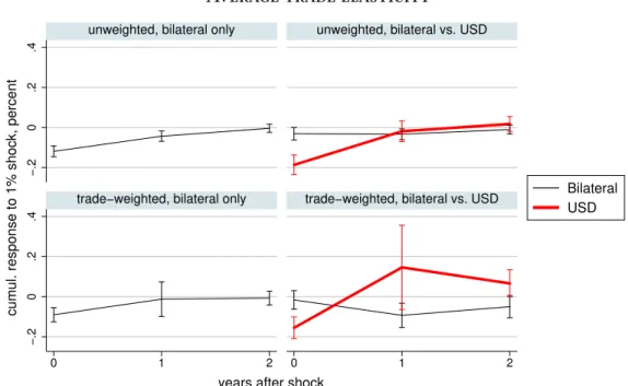
For our second finding, we estimate exchange rate pass-through and trade elasticity regressions
at the country-pair level. We first follow standard practice and estimate the pass-through ofbilateral exchange rates into import prices and volumes.3 We document that when country j’s currency depreciates relative to countryiby 10%, import prices in countryjfor goods imported from country
irise by 8%, suggestive of close to complete pass-through at the one year horizon. However, adding the U.S. dollar exchange rate as an additional explanatory variable and controlling for the global business cycle with time fixed-effects knocks the coefficient on the bilateral exchange rate from
0.76 down to 0.16. The coefficient on the dollar exchange rate of 0.78 largely dominates that of the
bilateral exchange rate. Moreover, the magnitude of the dollar pass-through is systematically related
to the dollar invoicing shares of countries. Specifically, increasing the dollar invoicing share by 10
3
This follows naturally from the classic Mundell-Fleming paradigm, according to which the price an importing country faces (when expressed in the importing country’s currency) fluctuates closely with the bilateral exchange rate. Accordingly, studies of exchange rate pass-through focus on trade-weighted or bilateral exchange rate changes (Goldberg and Knetter, 1997;Burstein and Gopinath,2014).
percentage points causes the contemporaneous dollar pass-through to increase by 3.5 percentage
points. Similar to the price regressions, adding the U.S. dollar exchange rate to a bilateral volume
forecasting regression knocks down the coefficient on the bilateral exchange rate by a substantial
amount. The contemporaneous volume elasticity for the dollar exchange rate is -0.19, while the
elasticity for the bilateral exchange rate is an order of magnitude smaller at -0.03.
These pass-through estimates point to a potential misspecification in the standard pass-through
regressions that ignore the role of the dollar. We also show that the dollar’s role as an invoicing
currency is indeed special, as it handily beats the explanatory power of the euro in price and volume
regressions. The data is also consistent with an additional key prediction of the dominant currency
paradigm: U.S. import prices and volumes are significantly less sensitive to the exchange rate, as
compared to other countries’ imports.
Third, we demonstrate empirically that the strength of the U.S. dollar is a key predictor of
rest-of-world (i.e. excluding the U.S.) trade volume and inflation, again controlling for measures of the
global business cycle. We find that a 1% appreciation of the U.S. dollar relative to all other
curren-cies is associated with a 0.6% contraction in rest-of-world aggregate import volume within the year.
Furthermore, countries with larger dollar import invoicing shares experience higher pass-through
of the dollar exchange rate into consumer and producer price inflation.
The global database has the advantage of covering almost all of world trade, but it is not at the firm
level and is only available at an annual frequency. We demonstrate that all our aggregate findings
hold also when we use firm-level data from Colombia, a small open economy that is representative
of emerging markets in its heavy reliance on dollar invoicing with 98% of exports invoiced in
dol-lars. Using prices and quantities defined at the firm-10-digit product-country (origin or
destination)-quarter (or year) level for manufactured goods (excluding petrochemical and basic metal industries),
we confirm that the U.S. dollar exchange rate knocks down the bilateral exchange rate for price pass
through and trade elasticity of exports and imports to/from non-dollarized economies. Further, we
To further contrast the different pricing paradigms, we simulate a model economy that is subject
to commodity price shocks, productivity shocks, and third country exchange rate shocks, all
cal-ibrated to Colombia, and test its ability to match the data. Using a combination of calibration and
estimation, we document that the data strongly rejects PCP and LCP in favor of DCP. We demonstrate
that all features of DCP matter for quantitatively matching the facts, including strategic
complemen-tarities in pricing and imported input use. Under our benchmark DCP specification we find, in line
with the data, the export pass-through at four quarters to both dollar and non-dollar destinations
to be 65%. Instead, when we shut down strategic complementarities and imported input use, the
predicted pass-through declines by half to 30%.
Related literature. Our paper is related to a relatively small literature that models dollar pricing. These includeCorsetti and Pesenti(2005),Goldberg and Tille(2008),Goldberg and Tille(2009),
De-vereux et al.(2007),Cook and Devereux(2006) andCanzoneri et al.(2013). All of these models, with
the exception ofCanzoneri et al.(2013), are effectively static with one-period-ahead price stickiness.
UnlikeCanzoneri et al.(2013), we explore a three region world, which is crucial to analyze differences
between dominant and non-dominant currencies.Goldberg and Tille(2009) explore three regions but
in a static environment. In addition, the dollar pricing literature assumes constant desired mark-ups
and production functions that use only labor.
Our contribution to this literature is two-fold. Firstly, we develop a new Keynesian open economy
model that combines dynamic dominant currency pricing, variable mark-ups and imported input
use in production. We develop testable implications and demonstrate the differential transmission of
monetary policy shocks across countries. Secondly, we empirically evaluate the dominant currency
paradigm using two novel databases described previously.
Our empirical evidence on the terms of trade is related toObstfeld and Rogoff(2000), who
con-duct one of the earliest tests of the Mundell-Fleming paradigm against the Betts-Devereux-Engel
and the trade-weighted exchange rate for 21 countries, using quarterly data for 1982-1998. They
report an average correlation of 0.26, which they interpret as a rejection of local currency pricing.
Even though the correlation is well less than 1, which would lend weak support for producer
cur-rency pricing, they conjecture that the low correlation could be because of the construction of the
trade-weighted exchange rates and/or because their terms of trade measures include commodity
prices. With the help of our globally representative data set, we improve uponObstfeld and Rogoff
(2000) in several dimensions. Specifically, we examine the bilateral terms of trade, excluding com-modity prices and we estimate pass-through coefficients as opposed to correlations. Moreover, we
test additional predictions of the different pricing paradigms.
Our exchange rate pass-through analysis is among the first to exploit a globally representative
data set on bilateral trade volumes and values. To our knowledge, the only other work that utilizes a
similarly rich data set isBussi`ere et al.(2016), who analyze trade prices and quantities at the product
level.4
The remaining literature on exchange rate pass-through falls into two main camps. First, many
papers use unilateral (i.e., country-level) time series, which limits the ability to analyze cross-sectional
heterogeneity and necessitates the use of trade-weighted rather than truly bilateral exchange rates
(e.g.,Leigh et al.,2015). Second, a recent literature estimates pass-through of bilateral exchange rates
into product-level prices, as opposed to unit values, but these micro data sets are available for only
a few countries (see the review byBurstein and Gopinath,2014).
The evidence on asymmetric responses of the volume of exports and imports is consistent with
that documented by Alessandria et al.(2013) for exports and Gopinath and Neiman (2014) for
im-ports.5
4
The goal of that paper is to quantify the elasticity of prices and quantities to the bilateral exchange rate and check if Marshall-Lerner conditions hold. In contrast, our goal is to empirically evaluate the predictions of the various pricing paradigms and in the process highlight the dollar’s central role in global trade.
5
The typical explanations for the sluggish export response relies on quantity frictions arising from sunk or search costs under PCP. DCP, consistent with the data, predicts that such relative prices are stable and therefore, does not require quantity frictions in the short-term to generate slow adjustments in exports.
Outline. Section 2presents the DCP model, proposes testable implications, and contrasts the trans-mission of monetary policy shocks across pricing paradigms. Section 3empirically tests the
impli-cations derived inSection 2using the global database. Section 4tests and estimates the model using
the Colombian micro data. Section 5concludes.
2
Model
Consider an economyj that trades goods and assets with the rest of the world. The nominal bilateral exchange rate between country j and another country i is denotedEij, expressed as the price of currency i in terms of currency j. We assume that the U.S. dollar is the dominant currency and let E$j denote the price of a U.S. dollar in currency j. An increase in Eij (resp. E$j) represents a depreciation of countryj’s currency against that of countryi(resp. the dollar).
As in the canonical open economy framework ofGal´ı (2008), firms adjust prices infrequently `a laCalvo. However, we depart fromGal´ı(2008) along four dimensions. First, we nest three different pricing paradigms: producer currency pricing, local currency pricing as well as dominant currency
pricing. Second, the production function uses not just labor but also intermediate inputs produced
domestically and abroad. Third, we allow for strategic complementarity in pricing that gives rise to
variable, as opposed to constant, mark-ups. Last, international asset markets are incomplete with
only risk-less bonds being traded, while Gal´ı (2008) assumes complete markets. We describe the
details below.
2.1
Households
Countryj is populated with a continuum of symmetric households of measure one. In each period householdhconsumes a bundle of traded goodsCj,t(h). Each household also sets a wage rateWj,t(h) and supplies an individual variety of labor Nj,t(h) in order to satisfy demand at this wage rate. Households own all domestic firms. To simplify exposition we omit the indexation of households
when possible. The per-period utility function is separable in consumption and labor and given by, U(Cj,t, Nj,t) = 1 1−σc C1−σc j,t − κ 1 +ϕN 1+ϕ j,t (1)
where σc > 0 is the household’s coefficient of relative risk aversion, ϕ > 0 is the inverse of the Frisch elasticity of labor supply andκscales the disutility of labor.
The consumption aggregator Cj,t is implicitly defined by a Kimball (1995) homothetic demand aggregator: X i 1 |Ωi| Z ω∈Ωi γijΥ |Ωi|Cij,t(ω) γijCj,t dω= 1. (2)
InEq. (2),Cij,t(ω)represents the consumption by households in countryj of varietyωproduced by countryiat timet.γij is a set of preference weights that captures home consumption bias in country
j, withP
iγij = 1, while|Ωi| is the measure of varieties produced in countryi. The functionΥ(.) satisfies the constraints Υ (1) = 1, Υ0(.) > 0 and Υ00(.) < 0. As is well-known, this demand structure gives rise to strategic complementarities in pricing and variable mark-ups. It captures the
classic Dornbusch(1987) andKrugman (1987) channel of variable mark-ups and pricing-to-market
as described below.
Households in countryj solve the following dynamic optimization problem,
max Cj,t,Wj,t,B$j,t+1,Bj,t+1(s0) E0 ∞ X t=0 βtU(Cj,t, Nj,t), (3)
where Et denotes expectations conditional on information available at time t, subject to the
per-period budget constraint expressed in home currency,
Pj,tCj,t+E$j,t(1 +i$j,t−1)B $ j,t+Bj,t = Wj,t(h)Nj,t(h) + Πj,t (4) +E$j,tBj,t$ +1+ X s0∈S Qj,t(s0)Bj,t+1(s0).
In this expression,Pj,t is the price index for the domestic consumption aggregatorCj,t. Πj,t repre-sents domestic profits transferred to domestic households, owners of domestic firms. On the financial
in-terest ratei$ j,t.
6
Bj,t$ +1 denotes the dollar debt holdings of this bond at timet. They also have access to a full set of domestic state contingent securities (inj currency) that are traded domestically and in zero net supply. DenotingS the set of possible states of the world,Qj,t(s)is the period-t price of the security that pays one unit of home currency in periodt+ 1and states ∈ S, andBj,t+1(s)are the corresponding holdings.
The optimality conditions of the household’s problem yield the following demand system:
Cij,t(ω) = γijψ Dj,t Pij,t(ω) Pj,t Cj,t, (5) whereψ(.) := Υ0−1(.)>0so thatψ0(.)<0,Dj,t :=P i R ΩiΥ 0|Ωi|Cij,t(ω) γijCj,t C ij,t(ω) Cj,t dω is a demand
index and Pij,t(ω) denotes the price of variety ω produced in country i and sold in country j, in currencyj. Define the elasticity of demandσij,t(ω) := −∂logCij,t(ω)
∂logZij,t(ω)
, whereZij,t(ω) := Dj,tPij,t(ω) Pj,t
.
The log of the optimal flexible price mark-up isµij,t(ω) := log
σij,t
σij,t−1
. It is time-varying and we
let Γij,t(ω) := ∂µij,t ∂logZij,t(ω)
denote the elasticity of that markup. By definition, the price index Pj,t satisfiesPj,tCj,t =P
i
R
ΩiPij,t(ω)Cij,t(ω)dω.
Inter-temporal optimality conditions for international and domestic bonds are given by the usual
Euler equations: C−σc j,t =β(1 +i $ j,t)Et C−σc j,t+1 Pj,t Pj,t+1 E$j,t+1 E$j,t (6) C−σc j,t =β(1 +ij,t)Et C−σc j,t+1 Pj,t Pj,t+1 (7) where(1 +ij,t) = (P
s0∈S Qj,t(s0))−1 is the inverse of the price of a nominally risk-freej-currency bond at timetthat delivers one unit ofj currency in every state of the world in periodt+ 1.
Households are subject to a Calvo friction when setting wages inj-currency: in any given period, they may adjust their wage with probability1−δw, and maintain the previous-period nominal wage otherwise. As we will see, they face a downward sloping demand for the specific variety of labor
they supply given byNj,t(h) =
W
j,t(h)
Wj,t
−ϑ
Nj,t, whereϑ >1is the elasticity of labor demand and
6
This dollar interest rate can be country specific, hence the dependency onjto reflect country risk premia, financial frictions or to ensure stationarity of the linearized model.
Wj,t is the aggregate nominal wage in countryj, defined below. The standard optimality condition for wage setting is given by:
Et ∞ X s=t δsw−tΘj,t,sNj,sW ϑ(1+ϕ) j,s " ϑ ϑ−1κPj,sC σ j,sN ϕ j,s− ¯ Wj,t(h)1+ϑϕ Wj,sϑϕ # = 0, (8) whereΘj,t,s := βs−t C −σc j,s C−j,tσc Pj,t Pj,s
is the stochastic discount factor between periodstands ≥ t used to discount profits andW¯j,t(h)is the optimal nominal reset wage in periodtand countryj. This implies thatW¯j,t(h)is preset as a constant mark-up over the expected weighted-average of future marginal rates of substitution between labor and consumption and aggregate wage rates, during the duration
of the wage. Sticky wages are useful to match the empirical fact that wage-based real exchange rates
move closely with the nominal exchange rates.
2.2
Producers
Each producer inj manufactures a unique variety ω, which is sold both domestically and interna-tionally. The output of the firm is used both for final consumption and as an intermediate input for
production. The production function uses a combination of laborLj,tand intermediate inputs Xj,t, with a Cobb Douglas production function:
Yj,t =eaj,tL1−j,tαXj,tα (9)
whereαis the share of intermediates in production andaj,t is an aggregate productivity shock. The intermediate input aggregatorXj,ttakes the same form as the consumption aggregator inEq. (2):
X i 1 |Ωi| Z ω∈Ωi γijΥ |Ω i|Xij,t(ω) γijXj,t dω= 1, (10)
whereXij,t(ω)represents the demand by firms in countryj for varietyω produced in countryias intermediate input. The labor inputLj,t is a constant elasticity aggregator of the individual varieties
Lj,t(h)supplied by each household,Lj,t =
h
R1
0 Lj,t(h)
(ϑ−1)/ϑdhiϑ/(ϑ−1),withϑ >1.
in each country i and the demand for domestic individual varieties (both for consumption and as intermediate input) takes a form similar to that inEq. (5).
Markets are assumed to be segmented so firms can set different prices by destination market and
invoicing currency. Denote Pk
ji,t(ω)the price of a variety ω originating inj, sold in countryi and invoiced in currencyk. The per-period nominal profits of the domestic firm producing varietyωare then given by:
Πj,t(ω) = X i,k Ekj,tPji,tk (ω)Y k ji,t(ω)− MCj,tYj,t(ω) (11) with the convention thatEjj,t:= 1. In that expression,Yji,tk (ω) = Cji,tk (ω) +Xji,tk (ω)is the demand for domestic variety ω from country j invoiced in currency k in country i, both for consumption and as an input in production, whileYj,t(ω) = P
i,kY k
ji,t(ω)is the total demand across destination markets iand invoicing currenciesk. MCj,t denotes the nominal marginal cost of countryj firms in their home currency. GivenEq. (9), it is given by:
MCj,t = 1 αα(1−α)1−α · Wj,t1−αPj,tα eaj,t . (12)
The optimality conditions for hiring labor are given by,
(1−α)Yj,t Lj,t = Wj,t MCj,t, Lj,t(h) = Wj,t(h) Wj,t −ϑ Lj,t, (13)
with the aggregate nominal wage Wj,t defined asWj,t = R Wj,t(h)1−ϑdh
1
1−ϑ, while the demand
for intermediate inputs is determined by,
αYj,t Xj,t = Pj,t MCj,t , Xij,t(ω) =γijψ Dj,t Pij,t(ω) Pj,t Xj,t. (14)
2.3
Pricing
Firms choose prices at which to sell injand in international marketsi, with prices reset infrequently. As inGal´ı(2008), we consider a Calvo pricing environment where firms are randomly allowed to reset
choices by firms, in particular under dominant currency pricing. Consequently, we assume that
firms can set their prices either in the producer currency (j), in the destination currency (i), or in the dominant currency ($).
Denoteθk
ji the fraction of exports from region j to regionithat are priced in currency k, with
P
kθ k
ji = 1 for any pair {i, j}. We allow for all pricing combinations but will focus on subsets. The benchmark of PCP corresponds to the case where θj
j,i = 1 for everyi 6= j. The case of LCP corresponds toθiji = 1for everyi 6=j. Under DCP,θ$ji = 1for everyi6= j. Lastly, we assume that all domestic prices are sticky in the home currency, an assumption consistent with a large body of
evidence: θj
jj = 1for everyj.
Consider the pricing problem of a firm from countryj selling in countryiand invoicing in cur-rencyk, and denoteP¯ji,tk (ω)its reset price. This reset price satisfies the following optimality condi-tion: Et ∞ X s=t δsp−tΘj,t,sYji,sk |t(ω)(σ k ji,s(ω)−1) Ekj,sP¯ji,tk (ω)− σkji,s(ω) σkji,s(ω)−1MCj,s ! = 0. (15) In this expression, Yk
ji,s|t(ω)is the quantity sold in country iinvoiced in currency k at times by a firm that resets prices at time t ≤ s and σkji,s(ω) is the elasticity of demand. This expression im-plies thatP¯k
ji,t(ω)is preset as a markup over expected future marginal costs expressed in currencyk, MCj,s(ω)/Ekj,s, over the duration of the price spell. Observe that because of strategic complemen-tarities, the mark-up over expected future marginal costs is not constant.
2.4
Testable Implications
Before we close the model, we can already outline a number of testable implications of our framework
for the joint behavior of exchange rates, export and import prices, and quantities. We explore them
empirically inSection 3.
inflation for goods originating from countryican be expressed as: ∆pij,t = X k θijk ∆pkij,t+ ∆ekj,t ,
where the summation is over invoicing currencies. Under Calvo pricing,∆pkij,t = (1−δp) ¯pkij,t−pkij,t−1, andp¯kij,tis the (log) reset-price defined inEq. (15). If all goods fromitoj are either producer-priced (PCP), locally-priced (LCP) or priced in the dominant currency (DCP), θi
ij +θ j ij +θ $ ij = 1 and we obtain: ∆pij,t =θiji ∆eij,t+θ$ij∆e$j,t + (1−δp) X k θkij p¯kij,t−pkij,t−1. (16) In the very short run, δp → 1, and we can ignore the last term of the previous equation: changes in bilateral import prices and in the bilateral terms of tradeT OTij = Pij/(PjiEij)only depend on the bilateral nominal exchange rates, the dollar exchange rate, and the share of trade invoiced in
different currencies.
On the quantity side a log-linear approximation (around a symmetric steady state) of Eqs. (5)
and(14)yields,
∆yij,t= −σij(∆pij,t−∆pj,t) + ∆yj,td , whereσij is the elasticity of demand andyd
j,t is the (log) of aggregate demand in countryj.
Proposition 1 (pass-through). When prices are fully rigid and pre-determined in their currency of in-voicing (δp → 1), pass-through into bilateral import prices expressed in currencyj and quantities from
countryito countryj (controlling for destination pricespj,tand demandyj,td ) are given by:
∆pij,t = θiij∆eij,t+θij$∆e$j,t (17)
∆yij,t = −σij θiij∆eij,t+θij$∆e$j,t (18) • In the case of PCP,θi ij =θ j ji = 1and
∆pij,t = ∆eij,t, ∆pji,t =−∆eij,t ∆totij,t = ∆pij,t−(∆pji,t+ ∆eij,t) = ∆eij,t.
• In the case of LCP,θjij =θjii = 1and
∆pij,t = 0, ∆pji,t = 0
∆totij,t = ∆pij,t−(∆pji,t+ ∆eij,t) =−∆eij,t ∆yij,t = 0.
• In the case of DCP,θij$ =θji$ = 1and
∆pij,t = ∆e$j,t, ∆pji,t = ∆e$i,t ∆totij,t = ∆pij,t−(∆pji,t+ ∆eij,t) = 0
∆yij,t = −σij,t∆e$j,t.
It should be clear that the predictions for prices, when prices are yet to change, do not depend
on what drives the exchange rate variation, that is, whether it arises from monetary policy shocks,
financial shocks or other shocks. Empirically, we should expect those countries relying more heavily
on dollar pricing to display greater sensitivity to the dollar exchange rate, even when controlling for
the bilateral exchange rate between countriesi andj.7 We summarize the testable implications of DCP below.
Testable Implications. (Import Price and Quantity Pass-Through)
1. The bilateral terms of trade should be insensitive to bilateral exchange rates.
2. For non-U.S. countries exchange rate pass-through into import prices (in home currency) should be high and driven by the dollar exchange rate as opposed to the bilateral exchange rate. Countries that rely more heavily on dollar import invoicing should see more of this effect. For the U.S., on the contrary, pass-through into import prices should be low.
3. For non-U.S. countries, import quantities should be driven by the dollar exchange rate as opposed to the bilateral exchange rate. U.S. import quantities should be less responsive to dollar exchange rate movements as compared to non-U.S. countries.
7
Note that if the source of the shock generates co-movement across exchange rates, the resulting collinearity would show up in the regressions as large standard errors around the point estimates on each bilateral exchange rate. As we report below, this is not an issue.
4. When all countries’ currencies uniformly depreciate relative to the dollar, it should lead to a decline in trade between the rest of the world (i.e. excluding the U.S.).
The first three implications follow directly fromProposition 1. The last implication is obtained
from the aggregation of import volumes across country-pairs where the U.S. is neither the origin nor
the destination country. DenoteR the set of such country-pairs: R ≡ {(i, j), i 6= j, i 6= $, j 6= $}.
Letωij denote countryj total non-commodity import value from countryiin some reference year, normalized so that P
Rωij = 1. We conceptualize the rest-of-the-world aggregate trade bundle,
yR,t, as a Cobb-Douglas aggregate of individual-country bilateral (log) gross imports with weights
ωij: y R,t :=
P
Rωijyij,t. Ceteris paribus, under DCP, a uniform depreciation relative to the dollar ∆e$,t >0, leads to a decline in non-commodity trade in the rest of the world:
∆yR,t= X R ωij∆yij,t=− X R ωijσij,t ! ∆e$,t<0. (19)
Under either PCP or LCP, the growth of the rest-of-the-world trade is instead∆y
R,t = 0, either be-cause bilateral non-dollar exchange rates are unchanged (under PCP) or bebe-cause there is no bilateral
pass-through (LCP).
As the horizon increases, the frequency of price adjustment increases and the pass-through
pre-dictions depend also on the response of reset pricesp¯kij,t to exchange rates. We demonstrate in Sec-tion 4.2 that the divergent predictions across the different paradigms hold at longer than annual
frequencies in the presence of strategic complementarities in pricing and imported input use.8
8
This result does not depend on the exogeneity of the currency of invoicing. Some of the ingredients from our model, namely imported input use in production and strategic complementarities in pricing, are precisely those that would give rise endogenously to dominant currency in pricing. This is demonstrated byGopinath et al.(2010) in a partial equilibrium environment andMukhin(2018) in a general equilibrium environment. Nonetheless, our testable predictions continue to hold, even after endogenizing the currency choice: as shown inGopinath et al.(2010), firms choose to price in currencies in which their reset prices are most stable, i.e., desired medium-run pass-through into the price (expressed in the invoicing currency) is low. In other words, our empirical findings will continue to be relevant in an environment with endogenous currency choice.
Lastly, as the horizon increases the impact of exchange rate fluctuations on prices and quantities depend on the source of the shock. The ideal test would be to examine the joint response of exchange rates, prices, and quantities to an exogenous shock such as a monetary policy shock. The problem is that in the data exchange rate fluctuations have little to do with monetary policy shocks or other identified policy shocks. Instead exchange rates appear to be driven by a ‘residual’ that the literature names ‘financial shocks.’ Practically this shows up as low power in testing the channel from identified exogenous shocks to exchange rates and to trade.
2.5
Closing the Model and Contrasting Shock Transmission
Before turning to our empirical results, this subsection demonstrates the differential transmission of
monetary policy (MP) shocks across different pricing paradigms in a Small Open Economy (SOE).
Then, using a 3-country Large Open Economy (LOE) framework, it further documents the asymmetry
in monetary policy spillovers under DCP, depending on whether the MP shocks originate in the
dominant currency country or elsewhere. We show that when countries follow a Taylor rule: (i) The
inflation-output trade-off in response to a monetary policy shock for a small open economy worsens
under DCP relative to PCP. (ii) MP shocks in the dominant country have strong spillovers to MP in
the rest-of-the world and reduce rest-of-world and global trade, while MP shocks in non-dominant
currency countries generate only weak spillovers and little impact on world trade. Details of the
simulations are provided in an online appendix.
2.5.1 Closing the Model
To evaluate shock transmission, we need to close the model. This requires that in addition to the
equilibrium conditions specified inSection 2we spell out the processes for interest rates and impose
market clearing conditions. We assume that the nominal interest rate in each countryiis set by its monetary authority and follows a Taylor rule with inertia:
ii,t−i∗ =ρm(ii,t−1−i∗) + (1−ρm) (φMπi,t+φYy˜i,t) +εi,t.
In this expression,φM captures the sensitivity of policy rates to consumer price inflationπi,t = ∆ lnPi,t,φY measures the sensitivity to the output gapy˜i,t,ρm captures the inertia in setting policy rates, while the target nominal interest rate is assumed equal to the steady state international
bor-rowing ratei∗.εi,tevolves according to anAR(1)process,εi,t = ρεεi,t−1+mi,twheremi,tare serially independently distributed innovations.9
9
In Section 4.2we examine moments of the stationary distribution for a small open economy. As is well known, in the absence of further assumptions the SOE model just described when solved around a well behaved steady state with
β(1 +i∗) = 1is non-stationary in that the level of real debt and therefore other real variables are permanently changed
Goods, labor and domestic bond market-clearing conditions requireYi,t(ω) =P
j(Cij,t(ω) +Xij,t(ω)),
Ni,t =Li,t,andBi,t(s0) = 0,∀s0 ∈ S. The remaining market clearing conditions depend on whether we consider a small open economy (SOE) or a large open economy (LOE) environment. In the SOE
case, all foreign variables are taken as exogenous and not impacted by shocks in the SOE. In the LOE
case, we impose the additional requirement thatP jB
$
j,t = 0.
2.5.2 Calibration
Preference aggregator. We adopt theKlenow and Willis(2016) functional form for the demand functionΥ(.). This gives rise to the following demand for individual varieties:
Yij,t(ω)≡ Cij,t(ω) +Xij,t(ω) =γi
1 +lnσ−1
σ −lnZij,t(ω)
σ/
(Cj,t+Xj,t)
whereZij,t(ω) ≡ Dj,tPij,t(ω) Pj,t
as previously defined and σ andare two parameters that determine the elasticity of demand and its variability as follows:
σij,t(ω) = σ 1 +lnσ−1σ −lnZij,t(ω) , Γij,t(ω) = σ−1−lnσσ−1 +lnZij,t(ω) .
In a symmetric steady stateZij,t(ω) = (σ−1)/σ, the elasticity of demand isσwhile the elasticity of the mark-up isΓ = /(σ−1). Strategic complementarities and variable markups arise when >0, while= 0corresponds to the constant elasticity case.
Parameter values. Table 1lists parameter values employed in the simulation. The time period is a quarter. Several parameters are set to values standard in the literature (see e.g.,Gal´ı,2008). Following
Christiano et al.(2011) we set the wage stickiness parameterδw = 0.85corresponding roughly to a year and a half average duration of wages. The steady state elasticity of substitution between varieties
dollar interest rate in countryi6= $is an increasing function of its external debt,i$
i,t=i$,t+ψ(e(B
$
i,t+1/P$)−B¯$i−1) +$
i,t, whereψ > 0measures the responsiveness of the dollar rate to the country’s real dollar debt holdingsB$
i,t+1/P$where P$is exogenous from the SOE perspective. B¯$
i is the exogenous steady-state real dollar debt holdings. This is a standard assumption in the small open economy literature to induce stationarity in a log-linearized environment. Because of the dependence on aggregate debt individual households do not internalize the effect of their borrowing choices on the interest rate. In this section we study the impulse response to a small one time shock and consequently the model with or without the stationarity assumption delivers almost identical results, as also shown bySchmitt-Grohe and Uribe(2003).
Parameter values for calibrated model
Parameter Value Parameter Value
Household Preferences Demand
Discount factor β 0.99 Elasticity σ 2.00
Risk aversion σc 2.00 Super-elasticity 1.00
Frisch elasticity ofN ϕ−1 0.50 Home-bias γ 0.70
Disutility of labor κ 1.00 Rigidities
Labor demand elasticity ϑ 4.00 Wage δw 0.85
Steady state NFA B¯$ 0 Price δp 0.75
Production Monetary Rule
Intermediate share α 2/3 Inertia ρm 0.50
(log) Productivity a 1 Inflation sensitivity φM 1.5 Output gap sensitivity φY 0.50/4 Shock persistence ρε 0.50 SS. interest rate i∗ (1/β)−1
Table 1:Parameter values for calibrated model.
σ is assumed in the model to be the same across and within regions. Accordingly, we calibrate to an average of these elasticities measured in the literature. Specifically, Broda and Weinstein(2006)
obtain a median elasticity estimate of 2.9 for substitution across imported varieties, while Feenstra
et al.(2010) estimate a value close to 1 for the elasticity of substitution across domestic and foreign
varieties. Thus, we setσ = 2.
To parameterize , which controls the strength of the strategic complementarities, we rely on estimates from the micro pass-through literature that converges on very similar values forΓdespite the differences in data and methodology. FollowingAmiti et al.(2016),Amiti et al.(2014),Gopinath
and Itskhoki(2010) we setΓ = 1. Because in steady stateΓ =/(σ−1)this implies= 1. The home bias share is set to 0.7. This implies steady-state spending on imported goods in the consumption
bundle and intermediate input bundle equal to thirty percent.10
2.5.3 Small Open Economy
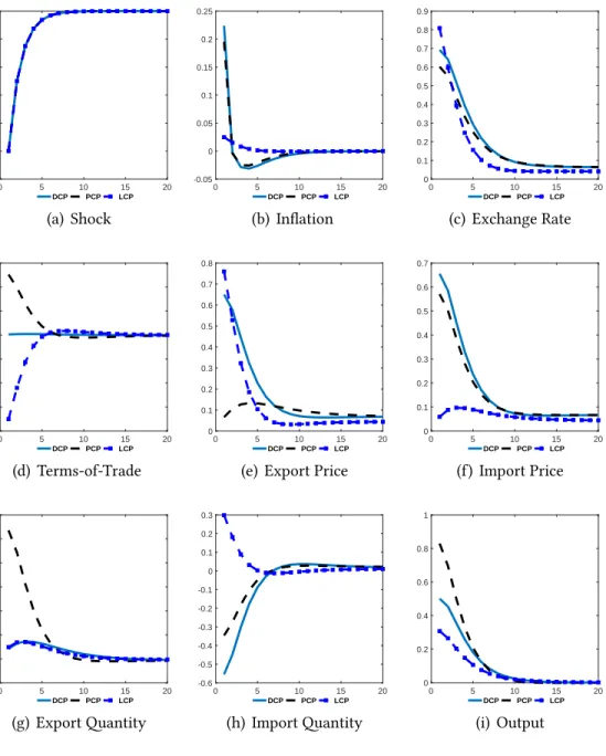
In this section we contrast the impulse responses to a monetary policy shock in a SOE (labeled H) under different pricing regimes. Fig. 1plots the impulse response to a25 basis point exogenous cut in
10
For the SOE case we assume exogenous rest-of-the world demand such that exports as a ratio of GDP is 45%. The specific value of this ratio is not essential to the results.
domestic interest rates (Fig. 1(a)). In each sub-figure, we contrast the response under three regimes: Dominant Currency Paradigm (DCP), Producer Currency Pricing (PCP), and Local Currency pricing
(LCP).
Exchange rate and inflation. Following the monetary shock, domestic interest rates decline but less than one-to-one as the exchange rateE$Hdepreciates by around 0.8% (Fig. 1(c)) raising inflation-ary pressures on the economy (Fig. 1(b)). This in turn dampens the fall in nominal interest rates via
the monetary policy rule. As seen inFig. 1(b)the increase in inflation in the case of DCP and PCP far
exceeds that of LCP since exchange rate movements have a smaller impact on the domestic prices of
imported goods when import prices are sticky in local currency.
Terms-of-trade. The exchange rate depreciation is associated with almost a one-to-one depreci-ation of the terms-of-trade in the case of PCP and a one-to-one apprecidepreci-ation in the case of LCP
(Fig. 1(d)). In contrast, under DCP, the terms-of-trade depreciate negligibly and remain stable
be-cause both export and import prices are stable in the dominant currency.
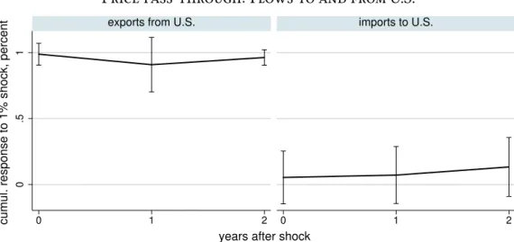
Exports and imports. With stable export and import prices in the dominant currency under DCP, the home currency price of exports and imports rises with the exchange rate depreciation as depicted
inFigs. 1(e)and1(f ). This in turn generates a significant decline in trade-weighted imports (0.43%),
despite the expansionary effect of monetary policy, and only a modest increase in trade-weighted
exports (0.1%) (Figs. 1(g) and1(h)). This contrasts with the PCP benchmark that generates a large
increase in exports and with the LCP benchmark that generates an increase in imports (from the
demand expansion). The decline in imports in the case of PCP is lower than that under DCP because
of export expansion under PCP and the use of imported inputs.
Output. As depicted inFig. 1(i)the expansionary impact on output is muted under DCP relative to PCP, with the lowest impact under LCP. Under DCP, there is an expenditure switching effect from
0 5 10 15 20 -0.3 -0.25 -0.2 -0.15 -0.1 -0.05 0 DCP PCP LCP (a) Shock 0 5 10 15 20 -0.05 0 0.05 0.1 0.15 0.2 0.25 DCP PCP LCP (b) Inflation 0 5 10 15 20 0 0.1 0.2 0.3 0.4 0.5 0.6 0.7 0.8 0.9 DCP PCP LCP (c) Exchange Rate 0 5 10 15 20 -0.8 -0.6 -0.4 -0.2 0 0.2 0.4 0.6 DCP PCP LCP (d) Terms-of-Trade 0 5 10 15 20 0 0.1 0.2 0.3 0.4 0.5 0.6 0.7 0.8 DCP PCP LCP
(e) Export Price
0 5 10 15 20 0 0.1 0.2 0.3 0.4 0.5 0.6 0.7 DCP PCP LCP (f ) Import Price 0 5 10 15 20 -0.2 0 0.2 0.4 0.6 0.8 1 1.2 DCP PCP LCP (g) Export Quantity 0 5 10 15 20 -0.6 -0.5 -0.4 -0.3 -0.2 -0.1 0 0.1 0.2 0.3 DCP PCP LCP (h) Import Quantity 0 5 10 15 20 0 0.2 0.4 0.6 0.8 1 DCP PCP LCP (i) Output
Figure 1:Impulse response to a monetary policy shock in a SOE
imports towards domestic output that is absent under LCP, while DCP misses out on the
expansion-ary impact on exports under PCP. Comparing Figs. 1(b) and 1(i), the inflation-output trade-off in
response to expansionary monetary policy worsens under DCP relative to both PCP and LCP (where
output does not expand much, but inflation increases the least). In the case of DCP, inflation rises by
0.35% on impact and output by 0.56%, a ratio of 0.4. In the case of PCP, that ratio is almost halved to
2.5.4 Large Open Economies
For the LOE case we consider three economies,U,GandR. These economies are symmetric, except for international pricing and bond markets in which the the dollar (the currency ofU) is dominant.11 Assuming 100% dollar pricing in international trade, we focus on the asymmetry in the transmission
of monetary policy shocks that originate inU, relative to those inG/R.
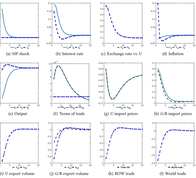
Monetary policy shock in dominant currency country. We first consider apositive 25 basis point shock to the nominal interest rate inU. The impulse responses to this monetary tightening are plotted in Fig. 2. The outcomes in G andRare the same for all variables, including their exchange rates, both of which depreciate by 0.65% relative to the dollar on impact.
The rise in interest rates inU leads to a decline in output (-0.6%, Figure 2(e)), an appreciation of the dollar (0.65%, Figure 2(c)), and a fall in inflation (-0.02%,Fig. 2(d)). The decline in inflation is,
however, negligible (in contrast to PCP) because dollar pricing generates a low pass-through of the
dollar appreciation into the price of imported goods, as seen in Fig. 2(g). On the other hand, the
pass-through into export prices (in the destination currency) is high, as depicted inFig. 2(h), which
in turn generates a significant decline in exports (Fig. 2(i)). Imports decline because of the decline
in overall demand given MP tightening so overall, the trade balance to GDP deteriorates mildly. The
terms of trade (Fig. 2(f )) are largely unchanged.
The monetary tightening inU has a larger effect on inflation on impact inG/R(0.2%,Fig. 2(d)) than inU because the depreciation has high pass-through into import prices of the former countries. This in turn generates an endogenous increase in interest rates (0.15%,Fig. 2(b)) inG/Rvia the Taylor rule, leading to a mild contraction in output (-0.03%, Fig. 2(e)). Despite the depreciation of theG/R exchange rates relative to the dollar, their exports toU decline (-0.4%,Fig. 2( j)) because dollar prices
11
We simulate the model also for the case when there is a full set of Arrow-Debreu securities traded. The impulse re-sponses, qualitatively and quantitatively, are very close. This is intuitive because under perfect foresight, the noncontingent bond is sufficient to complete the market, i.e., the equilibrium conditions of the cases with complete markets and incomplete markets with a bond are the same. When an unanticipated shock hits, only the initial period’s equilibrium conditions differ across the two cases.
toU change by little so there is no significant positive expenditure switching effect, and the decline in overall demand inU generates a decline in exports toU. Also, because of dollar pricing, there is a sharp decline in exports fromGtoR(-0.85%,Fig. 2( j)) and vice versa. This is because the depreciation of these countries’ currencies relative to the dollar makes all imports more expensive, leading to a
switch in expenditures away from imported goods. This is then further accentuated by the (mild)
negative impact on consumption from the rise in interest rates in response to the inflationary effect.
As follows from the previous discussion, a monetary tightening in U and the accompanying uniform appreciation of the dollar relative to other countries generate a decline in rest-of-world
trade (-0.83%, Fig. 2(k)), defined as the sum of quantities traded betweenG andR. It also causes a decline in global trade (-0.73%,Fig. 2(l)), defined as the sum of export quantities from all countries.
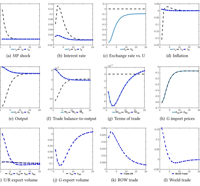
Monetary policy shock in non-dominant currency country. We next consider a25 basis point monetary tightening in a non-dominant currency country. Without loss of generality, we set this to be
G. As depicted in Fig. 3(c),G’s currency appreciates uniformly relative toU andRon impact, and by a magnitude similar to that inFig. 2(c). This is because, despite the endogenous change in interest
rates in each country (Fig. 3(b) differs from Fig. 2(b)), the change in the interest rate differential
between countries is quite similar, which is what matters for the exchange rate change.
The transmission of the shock to interest rates inG(Fig. 3(b)) is partly muted because the decline in inflation is endogenously contained through the Taylor rule. The negative impact on inflation of
-0.2% (Fig. 3(d)) contrasts with the much smaller effect of a MP shock inU onU’s inflation (Fig. 2(d)). This differential response arises from the strong pass-through of the appreciation of G’s currency into its import prices. The rise in interest rates in G leads to a decline in output (-0.6%, Fig. 3(e)). While pass-through into import prices (inG’s currency) is high (-0.6%,Fig. 3(h)), pass-through into export prices (in destination currency) is low. Consequently, there is only a small negative impact
on exports fromG(-0.05%,Fig. 3( j)), in contrast to the large negative impact of a MP tightening inU onU’s exports (Fig. 2(i)). While exports are not responsive, there is a significant increase in imports
0 5 10 15 20 -0.05 0 0.05 0.1 0.15 0.2 0.25 0.3 U G R (a) MP shock 0 5 10 15 20 -0.05 0 0.05 0.1 0.15 0.2 iU iG iR (b) Interest rate 0 5 10 15 20 0 0.1 0.2 0.3 0.4 0.5 0.6 0.7 eG eR (c) Exchange rate vs. U 0 5 10 15 20 -0.05 0 0.05 0.1 0.15 0.2 U G R (d) Inflation 0 5 10 15 20 -0.7 -0.6 -0.5 -0.4 -0.3 -0.2 -0.1 0 0.1 yU yG yR (e) Output 0 5 10 15 20 -2 0 2 4 6 8 10 10 -3
totGU totRU totGR
(f ) Terms of trade 0 5 10 15 20 -0.11 -0.1 -0.09 -0.08 -0.07 -0.06 -0.05 -0.04 pGU pRU (g) U import prices 0 5 10 15 20 0 0.1 0.2 0.3 0.4 0.5 0.6 0.7 pUG pUG (h) G/R import prices 0 5 10 15 20 -1 -0.8 -0.6 -0.4 -0.2 0 0.2 yUG yUR
(i) U export volume
0 5 10 15 20 -1 -0.8 -0.6 -0.4 -0.2 0 0.2 yGU yGR ( j) G/R export volume 0 5 10 15 20 -1 -0.8 -0.6 -0.4 -0.2 0 0.2 Trade GR (k) ROW trade 0 5 10 15 20 -0.8 -0.6 -0.4 -0.2 0 0.2 World trade (l) World trade
Figure 2: Impulse responses to a 25 basis point monetary tightening in U. Rest-of-world trade is defined as
the sum of quantities traded betweenGandR. World trade is defined as the sum of export quantities from all countries.
0 5 10 15 20 -0.05 0 0.05 0.1 0.15 0.2 0.25 0.3 U G R (a) MP shock 0 5 10 15 20 -0.02 0 0.02 0.04 0.06 0.08 0.1 0.12 0.14 iU iG iR (b) Interest rate 0 5 10 15 20 -0.7 -0.6 -0.5 -0.4 -0.3 -0.2 -0.1 0 0.1 eG eR (c) Exchange rate vs. U 0 5 10 15 20 -0.25 -0.2 -0.15 -0.1 -0.05 0 0.05 U G R (d) Inflation 0 5 10 15 20 -0.5 -0.4 -0.3 -0.2 -0.1 0 0.1 yU yG yR (e) Output 0 5 10 15 20 -15 -10 -5 0 5 10 -3 TBU TBG TBR (f ) Trade balance-to-output 0 5 10 15 20 -10 -8 -6 -4 -2 0 2 10 -3
totGU totRU totGR
(g) Terms of trade 0 5 10 15 20 -0.7 -0.6 -0.5 -0.4 -0.3 -0.2 -0.1 0 pUG pRG (h) G import prices 0 5 10 15 20 -0.1 0 0.1 0.2 0.3 0.4 0.5 0.6 yUG yUR yRU yRG
(i) U/R export volume
0 5 10 15 20 -0.12 -0.1 -0.08 -0.06 -0.04 -0.02 0 0.02 yGU yGR ( j) G export volume 0 5 10 15 20 0 0.005 0.01 0.015 0.02 0.025 0.03 Trade UR (k) ROW trade 0 5 10 15 20 -0.05 0 0.05 0.1 0.15 World Trade (l) World trade
Figure 3: Impulse responses to a 25 basis point monetary tightening in G. Rest-of-world trade is defined as
the sum of quantities traded betweenU andR. World trade is defined as the sum of export quantities from all countries.
intoGfromU, andRthrough the expenditure switching channel following the depreciation of their currencies relative toG’s (Fig. 3(i)). The terms of trade are stable, as in the case of the MP shock in
U (Fig. 3(g)).
Since exports from U and R to G increase significantly, while exports out of G decline only marginally, the monetary tightening inGis associated with an expansion in global trade (Fig. 3(l)), and almost no effect on rest-of-world trade (gross trade betweenU andR,Fig. 3(k)).
3
Global Empirical Evidence
This section tests the model predictions derived inSection 2.4, using bilateral trade volumes and unit
values for a large number of countries. We show that, consistent with DCP, the U.S. dollar plays an
outsized role in driving international trade prices and quantities. We first document that bilateral
terms of trade are essentially uncorrelated with bilateral exchange rates. Next, we demonstrate that
the bilateral (importer vs. exporter) exchange rates matter less than the exchange rate vis-`a-vis the
U.S. dollar for pass-through and trade elasticities of the average country in our sample. We also find
the euro to be much less important than the dollar. The effects of the dollar are stronger when the
importing country has a higher fraction of trade invoiced in dollars. The dollar’s role is greatest
for trade between emerging market pairs, consistent with their higher reliance on dollar pricing.
Finally, we show that the overall strength of the U.S. dollar is a key predictor of gross trade and
producer/consumer price inflation in the rest of the world.
3.1
Data
The core of our data set consists of panel data on bilateral trade values and volumes from Comtrade.
UN Comtrade provides detailed annual customs data for a large set of countries at the HS 6-digit
product level with information about the destination country, dollar value, quantity, and weight of
imports and exports. This dataset makes it possible to compute volume changes over time for each
chained Fisher price indices to aggregate up from the product level to the bilateral country level.
We focus entirely on data for non-commodity goods, except noted otherwise. Given the inherent
difficulty in drawing a line between commodities and non-commodities, we define commodities fairly
broadly as HS chapters 1–27 and 72–83, which comprise animal, vegetable, food, mineral, and metal
products.
The biggest challenge for constructing price and volume indices using customs data is the
so-called unit value bias. Unit values, calculated by dividing observed values by quantities, are not
actual prices. Even when there is no price change, unit values can change due to compositional
shifts. To take a stab at correcting for this bias, we follow the methodology developed byBoz et al.
(2019). Specifically, we eliminate 6-digit products with a unit value variance higher than a threshold
as those observations are more likely to be biased. To check whether this provides a sufficient fix,
we compare our Comtrade estimated price indices with those reported by the BLS based on actual
import prices for the U.S. We find that our indices track the BLS import price indices fairly well.
Results of this comparison, further details of Comtrade data construction as well as sources of other
macroeconomic data are provided in the online appendixA.1.
3.2
Terms of Trade and Exchange Rates
We first relate bilateral terms of trade to bilateral exchange rates using panel regressions (testable
implication 1). In this subsection, a cross-sectional unit is defined to be anunordered country pair, so that both trade flows between two countriesiandj are associated with the cross-sectional unit {i, j}. Recall thatpij denotes the (log) price of goods exported from countryito countryjmeasured in currencyj,eij the (log) bilateral exchange rate between countryiand countryj expressed as the price of currencyiin terms of currencyjandtotij = pij−pji−eij the (log) bilateral terms of trade, defined as the ratio of import prices to export prices (measured in the same currency). Moreover, let
ppiij denote the (log) ratio of the producer price index (PPI) in countryidivided by PPI in country
Terms of trade and exchange rates unweighted trade-weighted
(1) (2) (3) (4)
∆totij,t ∆totij,t ∆totij,t ∆totij,t ∆eij,t 0.0369*** -0.00938 0.0813*** 0.0218
(0.00863) (0.0130) (0.0235) (0.0317)
PPI no yes no yes
R-squared 0.008 0.011 0.028 0.042 Observations 24,270 19,847 24,270 19,847
Dyads 1,347 1,200 1,347 1,200
Table 2: The first (resp., last) two columns use unweighted (resp. trade-weighted) regressions. All regressions
include two∆ER lags and time FE. S.e. clustered by dyad. The number of dyads is about half that in Table3since here the two ordered country tuples(i, j)and(j, i)are collapsed into one cross-sectional unit{i, j}. *** p<0.01, ** p<0.05, * p<0.1.
We consider regressions of the following form:
∆totij,t =λij +δt+ 2 X k=0 βk∆eij,t−k + 2 X k=0
θk∆ppiij,t−k+εij,t, (20)
whereλij andδt are dyad (i.e., country pair) and time fixed effects. Regression Eq. (20)relates the growth rate of the bilateral terms of trade to the growth rate of the bilateral nominal exchange
rate (and lags). As discussed in Section 2.4, if exporting firms set prices in their local currencies as
in PCP and prices are sticky, the contemporaneous exchange rate coefficient β0 should equal 1. If instead exporting firms set prices in the destination currency as in LCP and prices are sticky, the
contemporaneous exchange rate coefficient should be−1. If most prices are invoiced in U.S. dollars and are sticky in nominal terms, the coefficientsβk should be close to zero. As indicated inEq. (20), some of our specifications control for lags 0–2 of the growth rate of the ratio of PPI in both countries,
since firms’ optimal reset prices should fluctuate with domestic cost conditions.
We consider both unweighted and trade-weighted regressions. To obtain trade weights, for each
dyad and year, we compute the share of world non-commodities trade value (in dollars) attributable
In line with DCP, we find that bilateral exchange rates are virtually uncorrelated with bilateral
terms of trade. The results of the panel regressions are shown in Table 2. If we do not control for
relative PPI, the regression results indicate that the contemporaneous effect of the exchange rate
on the terms of trade is positive. While the sign is consistent with PCP, the magnitude is not, as
the 95% confidence interval equals [0.02, 0.05] in the unweighted regression, and [0.04 , 0.13] in
the weighted regression.12 The coefficients on the lags (not reported) are also small in magnitude.
When controlling for relative PPI, the point estimates of the coefficients on the bilateral exchange
rate shrink further toward zero, and confidence intervals remain narrow. Hence, our results lend
strong support to DCP: the terms of trade are unresponsive to bilateral exchange rates.
Although the lack of correlation could in principle be consistent with a world of 50% PCP and
50% LCP, the next subsections refute that possibility. In addition, while the lack of correlation is
consistent with any currency being a dominant currency, we provide evidence next that the major
dominant currency is indeed the dollar. The stability of the terms of trade for the average country
in our sample cannot be explained by a model with flexible prices and strategic complementarities
in pricing as in Atkeson and Burstein(2008) andItskhoki and Mukhin (2017) because, as we show
next, the import pass-through into destination country prices at-the-dock is high, while that into
consumer or producer prices, reported in online appendix A.2.2, is an order of magnitude smaller,
contrary to the presence of strong complementarities in pricing.
Lastly, online appendixA.2.1demonstrates that the terms of trade are nearly uncorrelated with
the bilateral exchange rate across all advanced/emerging economy trade flows.
3.3
Exchange Rate Pass-through Into Prices
Next, we relate international prices and exchange rates (testable implication2). Exchange rate
pass-through regressions are reduced-form regressions that relate price changes to exchange rate changes
and other control variables relevant for pricing. We follow the literature and estimate the standard
12
Attenuation bias is not a worry in this context, since the explanatory variables of interest (exchange rates) are precisely measured, except perhaps for time aggregation issues at the annual frequency.
pass-through regression as described inBurstein and Gopinath(2014). In the rest of this section, the
cross-sectional unit is anorderedcountry pair(i, j). We estimate
∆pij,t =λij +δt+ 2 X k=0 βk∆eij,t−k+ 2 X k=0 βk$∆e$j,t−k (21) + 2 X k=0 ηk∆eij,t−k×Sj+ 2 X k=0 ηk$∆e$j,t−k ×Sj+θ0Xi,t +εij,t,
where λij and δt are dyadic and time fixed effects. Xi,t are other country i controls, namely the change in the (log) producer price index of the exporting countryimeasured in currencyi(and two lags).13 We have modified the textbook pass-through regression by including the dollar exchange
rate, i.e., the log price e$j of a U.S. dollar in currency j, alongside the bilateral exchange rate, as suggested inSection 2.4. Lastly, we interact the bilateral and dollar exchange rates with the importing
country’s dollar invoicing share Sj. We consider different versions of this general specification, omitting dollar exchange rates and/or interaction terms.
As a benchmark, the estimates from bilateral pass-through regressions on bilateral exchange rates
(i.e., omitting the dollar exchange rates and interaction terms) are reported in columns (1) and (4) of
Table 3. The two columns correspond to unweighted and trade-weighted regressions, respectively.14
According to the regression estimates, when countryj’s currency depreciates relative to countryi by 10%, import prices in country j rise by 8%, suggestive of close to complete pass-through at the one year horizon.15 The second and third lags (not reported) are economically less important.
Columns (2) and (5) report estimates from regressions that include the dollar exchange rate in
addition to the bilateral one. Including the dollar exchange rate sharply reduces the relevance of the
bilateral exchange rate. It knocks the coefficient on the bilateral exchange rate from 0.76 to 0.16 in
the unweighted regression, and from 0.77 to 0.34 in the weighted regression. Instead, almost all of
13
Online appendixA.2.5shows that our results are robust to adding importer PPI and GDP growth as additional control variables.
14
Henceforth, the trade weights are given by the average (across the years 1992–2015) share of world non-commodities trade value attributable to anordereddyad(i, j).
15
Exchange rate pass-through into prices
unweighted trade-weighted
(1) (2) (3) (4) (5) (6)
∆pij,t ∆pij,t ∆pij,t ∆pij,t ∆pij,t ∆pij,t
∆eij,t 0.757*** 0.164*** 0.209*** 0.765*** 0.345*** 0.445*** (0.0132) (0.0126) (0.0169) (0.0395) (0.0449) (0.0336) ∆eij,t×Sj -0.0841*** -0.253*** (0.0240) (0.0482) ∆e$j,t 0.781*** 0.565*** 0.582*** 0.120* (0.0143) (0.0283) (0.0377) (0.0622) ∆e$j,t×Sj 0.348*** 0.756*** (0.0326) (0.0796) R-squared 0.356 0.398 0.515 0.339 0.371 0.644 Observations 46,820 46,820 34,513 46,820 46,820 34,513 Dyads 2,647 2,647 1,900 2,647 2,647 1,900
Table 3: The first (resp., last) three columns use unweighted (resp. trade-weighted) regressions. All regressions
include two∆ER lags, lags 0–2 of exporter∆PPI, and time FE. S.e. clustered by dyad. *** p<0.01, ** p<0.05, * p<0.1.
the effect is absorbed by the dollar exchange rate.16 Notice that, due to our inclusion of time fixed
effects, the apparent dominance of the dollar cannot be an artifact of special conditions that may
apply in times when the dollar appreciates or depreciates against all other currencies, for example due to global recessions or flight to safety in asset markets. Online appendix A.2.5shows that our
results are robust to the choice of time sample, including removing the post-2008 period.
The cross-dyad heterogeneity in pass-through coefficients is related to the propensity to invoice
imports in dollars. Columns (3) and (6) interact the dollar and bilateral exchange rates with the share
of invoicing in dollars at the importer country level, as in regression Eq. (21). Notice that we do
not have data on the fraction ofbilateraltrade invoiced in dollars, so we use the importer’s country-level share as a proxy. As expected, the import invoicing share plays an economically and statistically
16
In the literature,unilateralexchange rate pass-through is sometimes estimated using a Vector Error Correction Model (VECM) that allows for cointegration between price levels and exchange rates. However,Burstein and Gopinath(2014, p. 403) find VECM results to be highly unstable across specifications, and this issue is likely to be compounded by measurement error in our bilateral data.