Inter-American Development Bank Banco Interamericano de Desarrollo (BID)
Research Department Departamento de Investigación
Working Paper #484
Sudden Stops and Exchange Rate Strategies
in Latin America
by
Arturo Galindo
Alejandro Izquierdo
Inter-American Development Bank
Cataloging-in-Publication data provided by the Inter-American Development Bank
Felipe Herrera Library
Galindo, Arturo.
Sudden stops and exchange rate strategies in Latin America / by Arturo Galindo, Alejandro Izquierdo.
p. cm. (Research Department Working paper series ; 484) Includes bibliographical references.
1. Foreign exchange rates--Latin America I. Izquierdo, Alejandro, 1964-. II. Inter-American Development Bank. Research Dept. III. Title. IV. Series.
332.456 G129---dc21
©2003
Inter-American Development Bank 1300 New York Avenue, N.W. Washington, D.C. 20577
The views and interpretations in this document are those of the authors and should not be attributed to the Inter-American Development Bank, or to any individual acting on its behalf. The Research Department (RES) produces the Latin American Economic Policies Newsletter, as well as working papers and books, on diverse economic issues.
To obtain a complete list of RES publications, and read or download them please visit our web site at: http://www.iadb.org/res
1. Introduction
1Recent crises in Latin America have motivated a lively debate over the choice of an exchange rate regime. It is standard in the profession to think about flexible exchange rates as the appropriate tool when the source of shocks comes from the real side of the economy, whereas fixed exchange rates are better suited for scenarios where monetary shocks are frequent. These views abstract from financial issues that have become quite relevant recently, namely, the effects of debt valuation and contingent liabilities on public sector sustainability following a sudden stop in capital flows.
Just like many other Emerging Markets (EMs), Latin American countries were hit hard by the capital flow standstill that followed the Russian crisis of August 1998. We argue that one of the main reasons why this unexpected stop in capital flows was so costly in some cases has a lot to do with the fact that this shock exposed many economies to substantial swings in the real exchange rate (RER). Some countries were more prepared than others to absorb this dramatic change in relative prices. We show that a large depreciation of the RER can lead to fiscal sustainability problems, particularly in relatively closed, highly indebted, heavily dollarized (and mismatched) emerging markets. Implicit in this line of reasoning is the fact that RER behavior may be highly influenced by capital account developments.
Given this context, we will explore the hypothesis that the choice of an exchange rate strategy following a sudden stop in capital flows (and the success of this strategy) may be influenced by the fiscal costs that countries have to face when the RER depreciates to its new equilibrium. In turn, these costs depend on a variety of initial conditions, which we explore in more detail below. When fiscal sustainability does not become an important issue, and in the absence of heavy liability dollarization that may lead to the materialization of contingent liabilities, it may be possible to accommodate the need for RER adjustment by allowing for higher flotation of the nominal exchange rate, coupled with a credible monetary policy rule, such as inflation targeting. But when fiscal sustainability is at stake, it may be very difficult to commit to a credible monetary policy, given that lack of access to capital markets at the time of a crisis may lead to the expectation that a series of liabilities will have to be monetized. In cases of extreme fiscal insolvency, it may even be necessary to surrender monetary policy (i.e., via
1 The authors work at the Research Department of the Inter-American Development Bank (IADB). They are
dollarization) at the same time that a fiscal adjustment or other solvency resolution mechanisms are implemented.
Drawing heavily on work by Calvo, Izquierdo and Talvi (2002),2 we argue that three characteristics make countries particularly vulnerable to a standstill in capital flows: 1) A small share of tradable goods output relative to domestic absorption of tradable goods, which, under certain conditions, leads to big swings in the RER; 2) Liability dollarization in non-tradable sectors (including the government), which makes them particularly vulnerable to big balance sheet effects following RER depreciation; and 3) High initial public debt levels, which may become unsustainable after an RER depreciation, particularly if debt is denominated in foreign currency.
Sometimes these weaknesses may remain hidden for a long period of time if the exchange rate is fixed or tightly managed (e.g., displaying Fear of Floating, see Calvo and Reinhart, 20023). As a result, politicians and the general public become largely unaware of the magnitude of the problem, thus undermining the political support for the necessary fiscal and financial adjustment and reform. We make particular emphasis on this point when we focus on Argentina’s response to the sudden stop.
In this context, we analyze policy decisions taken by a set of countries that underwent strong adjustment following the Russian crisis. We describe their ongoing exchange rate regimes, their response to the crisis, and their choice of a way out of the crisis, based on the fiscal and financial issues they faced. We also explore different measures of the success of their strategies in terms of output behavior, monetary outcomes, and their ability to compensate for the capital flow standstill by boosting other components of the balance of payments account, such as exports. In other words, we focus on the ability of countries to provide the right pricing information implicit in RER fluctuations, and their capacity to sustain credible monetary policies along the way.
The paper is organized as follows: section 2 describes the evolution of capital flows to Latin America after the Russian crisis and the countries’ response via current account adjustments. Section 3 presents a framework to measure the effects of sudden stops on the RER.
authors’ and do not necessarily reflect those of the Inter-American Development Bank.
2 See Guillermo Calvo, Alejandro Izquierdo and Ernesto Talvi, “Sudden Stops, The Real Exchange Rate and Fiscal
Sustainability: Lessons from Argentina,” Research Department Working Paper 469, Inter-American Development Bank.
Section 4 shows how Latin American countries responded to the capital shock and the real exchange adjustment in terms of their exchange rate policies, and identifies some of the reasons underlying the strategies that were adopted. Section 5 analyzes their degree of success. Section 6 studies the current exposure of the countries in our sample to a sudden stop. Section 7 concludes.
2. The World Scene after Russia
Russia’s August 1998 crisis has been a landmark in emerging capital markets. Massive capital inflows that set sail to Latin America in the early 1990s, financing high growth rates and large current account deficits, came all of a sudden to a standstill following Russia’s partial foreign debt repudiation in August 1998. It was a real challenge for analysts to imagine how a crisis in a country with little if any financial or trading ties to Latin America could have such profound effects on the region. This puzzle seriously questioned traditional explanations for financial crises (based on current account and fiscal deficits) and led to studies that focused on the intrinsic behavior of capital markets. In this respect, it was argued that prevailing rules for transactions at the heart of capital markets, such as margin credit, may have been responsible for the spread of shocks from one country to other regions (see, for example, Calvo, 19994).
Figure 1 shows bond spreads for EMs, which display a dramatic increase following the Russian crisis. Although they have since decreased, spreads exhibit a substantial gap compared to pre-crisis levels, exceeding 250 basis points for 2001.5 This gap was much higher for 1999 and 2000 (over 700 basis points and 300 basis points, respectively, as shown in Table 1).
3 Guillermo Calvo and Carmen Reinhart, 2002, “Fear of Floating,” forthcoming in Quarterly Journal of Economics. 4 Guillermo Calvo, 1999, “Contagion in Emerging Markets: When Wall Street is a Carrier,” mimeographed
document, University of Maryland. As the argument goes, to the extent that there exist large fixed costs (relative to the size of projects) in obtaining information about a particular country, resulting economies of scale lead to the formation of clusters of specialists, or informed investors, who lead capital markets. These investors leverage their portfolios to finance their investments and are subject to margin calls in the event of a fall in the price of assets placed as collateral. Remaining investors, the uninformed, observe transactions made by informed investors, but are subject to a signal-extraction problem, given that they must figure out whether sales of the informed are motivated by lower returns on projects or by the informed facing margin calls. As long as the variance of returns to projects is sufficiently high relative to the variance of margin calls, uninformed investors may easily interpret massive asset sales as an indication of lower returns and decide to get rid of their holdings as well, even though the cause for informed investors’ sales was indeed due to margin calls.
Figure 1. 400 600 800 1000 1200 1400 1600 1800 Ja n-9 8 Ap r-98 Ju l-9 8 Oct -98 Ja n-9 9 Ap r-99 Jul -9 9 Oct -99 Ja n-0 0 Ap r-00 Ju l-0 0 Oct -00 Jan-01 Ap r-01 Jul-01 Oc t-01 EMBI+ W/O Argentina
External Financial Conditions
(EMBI+, Spread over US Treasuries)
Source: JP Morgan Chase.
Table 1.
1999 2000 2001
EMBI + 666 307 393
EMBI + w/o Argentina 757 315 259
Source: JP Morgan Chase. Note: Values are yearly averages.
Difference in Bond Spreads with Minimum Pre-Crisis Levels
For most EMs, higher interest rates were accompanied by a large reduction in capital inflows. Latin American markets were no exception. Figure 2 and Table 2 show that the decline was sharp, particularly for portfolio flows, mimicking the sharp interest rate hike. The fact that the root of this phenomenon lay in Russia’s crisis indicates that the capital-inflow slowdown
contained a large unexpected component. “Large and unexpected” are the two defining characteristics of what the literature calls Sudden Stop (Calvo and Reinhart, 20006).
Figure 2. 0% 1% 2% 3% 4% 5% 6% 19 97-I V 19 98-I 19 98-II 19 98 -I II 19 98-I V 19 99-I 19 99-II 19 99 -I II 19 99-V 20 00-I 20 00-II 20 00 -I II 20 00-I V 20 01-I 20 01-II
Sudden Stop in LA 7 Biggest Economies
(Capital flows, % of GDP)
Source: Central Banks of Argentina, Brazil, Chile, Colombia, Mexico, Peru and Venezuela
Table 2.
1998.II 2001.III Reversal
Capital Flows 5.6 1.6 -4.0
Non-FDI Capital Flows 2.0 -0.9 -2.9
FDI 3.6 2.5 -1.1
Source: LA7 countries Central Banks.
Capital Flows, % of GDP, LA7 Biggest Economies
To the extent that the slowdown in capital flows was unexpected, it forced countries to a drastic adjustment of their current account deficits to accommodate the shortage of external
6 See Guillermo Calvo and Carmen Reinhart, 2000, “When Capital Flows Come to Sudden Stop: Consequences and
Policy” in Peter K. Kenen and Alexander K. Swoboda, editors, Reforming the International Monetary and Financial System, Washington, DC, United States: International Monetary Fund.
credit. Starting in the fourth quarter of 1998, key Latin American countries showed a steady decline in their current account deficit, which eventually reached a zero balance by the end of 2000.7 This adjustment of the current account was on average equivalent to 5 points of GDP for the seven biggest Latin American economies (see Figure 3).
Figure 3. -6% -5% -4% -3% -2% -1% 0% 1997 -I 19 97-I I 19 97 -I II 19 97-I V 1998 -I 19 98-II 19 98 -I II 19 98-I V 1999 -I 19 99-I I 19 99 -I II 19 99-V 2000 -I 20 00-I I 20 00 -I II 20 00-I V 2001 -I 20 01-II 20 01 -I II
Current Account in LA7 Biggest Economies
(4 quarters, % of GDP)
Source: Central Banks of Argentina, Brazil, Chile, Colombia, Mexico, Peru and Venezuela.
As shown in Table 3, this was a common response across individual countries. However the sharpness of the adjustment varies from case to case. For most countries the current account gap was closed within a year of the sudden stop, with the exception of Argentina and Brazil, who, for reasons that we will explore below, were not subject to such strong adjustment. For
7 Although FDI flows fell on average in the aftermath of the Russian crisis, they did increase significantly in Brazil,
where FDI flows rose 80 percent in dollar terms from the second quarter of 1998 to the second quarter of 2001. We follow up on this fact because it may be an important element behind the resumption of capital flows to Brazil. A possible explanation is that higher interest rates led to sharp declines in domestic collateral, adding to the perception that this asset class was more risky than expected. Thus, domestic firms found it more difficult to finance the current operations and expansion plans, further depressing their plants’ market value. This may have opened attractive investment opportunities for G7-based firms whose collateral was insulated from EM financial turmoil, leading to a sharp increase in FDI.
illustrative purposes, throughout the paper we have included Mexico’s 1994 sudden stop experience, although Mexico was not subject to a sudden stop after the Russian crisis.
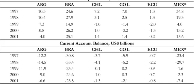
Table 3. Net Private Capital Flows and Current Account Balance
ARG BRA CHL COL ECU MEX*
1997 10.3 24.6 7.2 7.0 1.3 34.8
1998 10.4 27.9 3.1 2.5 1.3 19.3
1999 7.3 14.9 -1.0 -1.4 -2.0 4.0
2000 0.8 26.2 1.0 -0.2 -1.5 13.2
2001 -4.0 25.1 1.4 1.4 0.2 15.6
Current Account Balance, US$ billions
ARG BRA CHL COL ECU MEX*
1997 -12.2 -30.8 -3.7 -5.9 -0.7 -23.4
1998 -14.5 -33.4 -4.1 -5.2 -2.2 -29.7
1999 -11.9 -25.4 -0.1 0.2 0.9 -1.6
2000 -9.0 -24.6 -1.0 0.3 0.7 -2.3
2001 -6.6 -23.5 -1.3 -2.1 -0.8 -7.4
Source: World Economic Outlook (IMF), December 2001. */ Figures for Mexico are for the period 1993-97.
Net Private Capital Flows, US$ billions
3.
Sudden Stops and Real Exchange Rate Adjustment
So far we have made a case for the stalling of capital flows. But what are the consequences of this event in terms of RER behavior and debt sustainability analysis? Two key elements in this discussion are the unexpected component of the sudden stop and its duration. It is clear that expectations prevailing before the Russian crisis had not factored in the widespread effects on EMs that followed, so the unexpected element required for a sudden stop is met. A different question is whether this shock was perceived as temporary or highly persistent, which is quite relevant from a policy perspective. With the benefit of hindsight it is easy to argue that the shock had a large persistence component, since the stalling in capital inflows has lasted for more than three years. But it is not clear that it was perceived as such from the very beginning (this is an important point that we will revisit when we discuss Argentina in greater detail). Indeed, investors and policymakers had witnessed a quick recovery of capital flows following the Mexican crisis at the end of 1994, which could have led them to expect a similar quick recovery
after the Russian collapse. But things turned out to be different. Figure 4 shows that two years after the Mexican crisis there was more than a complete recovery of capital flows, whereas there has been no recovery in the region since the Russian crisis.
Figure 4. 35 40 45 50 55 60 65 70 75 T T+1 T+2 T+3 Tequila Russia
Sudden Stop in LAC
(Net private capital flows, US$ billions)
Note: “LAC” refers to Western Hemisphere countries, according to IMF definition.
“T” denotes the year of occurrence of the crisis. Source: World Economic Outlook (IMF), December 2001.
Sudden stops are typically accompanied by large contractions in international reserves
and declines in the relative price of non-tradables with respect to tradables (i.e., RER depreciation). To illustrate the effects on the RER, we present a framework developed in Calvo, Izquierdo and Talvi, 2002. Consider the case of a small open economy that experiences a current account deficit before a sudden stop takes place. By definition:
*, *
* S Y
A
CAD= + − (1)
where CAD is the current account deficit, A* is absorption of tradable goods, S* represents non-factor payments to foreigners, and Y* is the supply of tradable goods. If financing of the current account deficit is stopped, the full amount of that imbalance needs to be cut. A measure of the percentage fall in the absorption of tradable goods needed to restore equilibrium is given by:
, 1 *
/ ω
η =CAD A = − (2)
where ω is a measure of the un-leveraged absorption of tradable goods, defined as: . * / *) * (Y −S A = ω (3)
Notice that this measure captures the share of absorption of tradable goods that is financed by the supply of tradable goods.8 The lower this value, the higher will be the share of absorption of tradables financed from abroad. In other words, relatively closed economies with a small supply of tradable goods will be highly leveraged. As we will see later, this is an important consideration regarding RER behavior after a sudden stop in capital flows.
Table 3 shows that the current account adjustment was sharp in most cases. Indeed, it is not uncommon to see an abrupt adjustment towards current account balance within a year following the sudden stop.
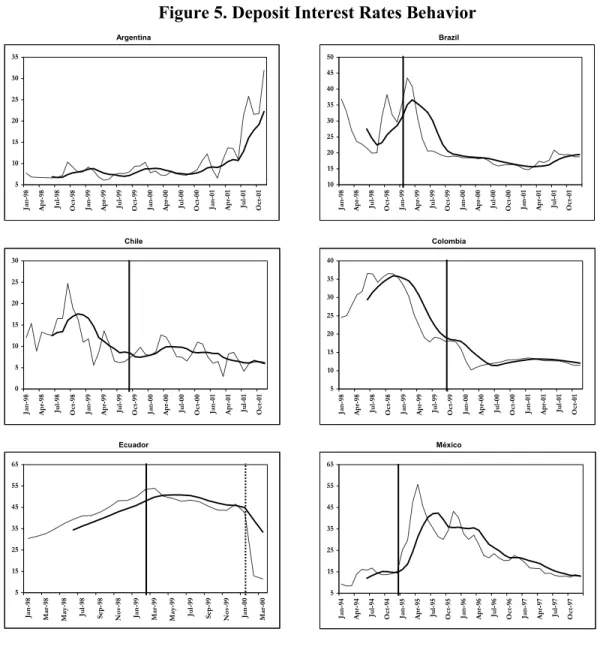
In order to obtain an estimate for η that can be used for cross-country comparisons, we proxy A* with imports. We use the observed current account adjustment for different periods, taken as a share of imports at the time of the crisis, in order to illustrate the observed percentage fall in absorption of tradable goods. Results are shown in Table 4 for 1999 and 2001. Countries like Chile, Colombia, and Ecuador, where the percentage fall ranged anywhere from 18 to 49 percent, experienced a quick and substantial adjustment in absorption of tradable goods by 1999.9 Adjustment in Brazil and Argentina has taken longer, a phenomenon that we will analyze in more detail later.
Table 4.
ARG BRA CHL COL ECU MEX*
1999 vs 1998 6.1 10.6 18.8 31.3 49.0 39.5
2001 vs 1998 18.7 13.1 13.1 18.0 21.3 31.2
Source: World Economic Outlook (IMF), December 2001. */ Figures for Mexico are for the period 1994-97.
Current Account Change, % of 1998 Imports
8 Net of non-factor payments.
Having shown that the percentage fall of tradable goods absorption can be substantial after a sudden stop, we now consider effects on non-tradable goods. A common assumption in the literature is that preferences are homothetic, implying that the income expansion path of tradable vis-à-vis non-tradable goods is linear. Under this assumption, given an RER, consumption of non-tradable goods is therefore proportional to that of tradable goods.10 As a result, a decline in demand for tradable goods of size η must be matched by a proportional fall of equal size in the demand for non-tradable goods. Now consider the effects of this fall in demand on the RER. Given that the price of tradable goods is determined from abroad, all we need to take into account is the behavior of the tradable goods market. Define demand for non-tradables as:
,
p a
h= −χ (4)
where h is (the log of) demand for non-tradable goods, and p is (the log of) the relative price of non-tradable to that of tradable goods, i.e., the inverse of the RER. Then, for a given RER, the fall in demand following a sudden stop is simply:
.
1 ω
η= − =
da (5)
Assuming, for simplicity, that the supply of non-tradable goods is fixed (so that dh = 0), then the required percentage change in the real exchange, after differentiation of (4), is given by:
; / ) 1 ( −ω χ = dp (6)
that is to say, the more closed an economy is in terms of its supply of tradables,11 relative to absorption of tradables, the higher the impact on the RER needed to restore equilibrium after a sudden stop. The intuition for this result is that, in the short run, the ability to generate purchasing power in terms of tradables is exports minus debt service. Thus, a Sudden Stop that requires a greater external surplus implies a larger proportional sacrifice in absorption in terms of tradables, the smaller is ω. Another element that affects our measure of un-leveraged
10 In what follows we abstract from investment. This is indeed a major omission, which is, however, likely to be
less misleading in a steady state context such as the present one. Catena and Talvi (2001) reach similar results in terms of a full-fledged dynamic model. See Marcelo Catena and Ernesto Talvi, 2001, “Sudden Stops in a Dynamic General Equilibrium Model: An Application to Latin American Countries,” mimeographed document.
absorption is non-factor payments (S*), typically composed of interest payments, which implicitly captures indebtedness levels. High indebtedness therefore reduces available resources to finance absorption of tradable goods, requiring greater RER realignment following a standstill in capital flows. Given these characteristics, ω is a good summary statistic to measure the impact on RER realignment. A further simplifying assumption is that the supply of tradable goods can be measured by exports whereas, as earlier noted, imports serve as a proxy for absorption of tradables.12 Table 5 contains a list of Latin American EMs ranked by this measure in 1998.13 Chile clearly leads the ranking in terms of openness. Argentina, although not the lowest ranked in the group, stands 15 percentage points below Chile, indicating that it would need greater RER realignment following a sudden stop.
Table 5.
BRA MEX* ARG ECU COL CHL
0.56 0.58 0.66 0.66 0.70 0.81
Source: World Economic Outlook (IMF), and own estimates. Note: This measure is calculated in 1998 for all countries, except for Mexico (1994).
Un-leveraged Absorption Coefficient (ω)
Another key element in determining the size of the required change in the RER is given by the price elasticity of the demand for home goods, χ. Estimates for developing countries are much lower than those for industrial countries, implying that sudden stops can be much more devastating for EMs. Thus, not only are sudden stops a much more common feature of developing countries, but their effects can be more dangerous as well. Actually, the higher vulnerability of EMs to sudden stops could partly explain their higher recurrence.
Given this framework, we ask next what should be the size of RER realignment following a sudden stop that requires a full adjustment of the current account deficit, using 1998 as a starting point. To compute this, we make use of equation (6), taking a value of χ = 0.4 (the lower bound of the literature). Given that we measure the RER as the inverse of p, we compute the rate of depreciation for 1/p. Obviously, these figures should not be taken at face value, but as
12 A scenario which is more plausible in the short run. 13 Except for Mexico, where values are computed for 1994.
a way of ranking the effects of a sudden stop across countries.14 Table 6 shows the results. As it stands, this exercise would indicate that Argentina would have needed to depreciate its RER by 46 percent in order to bring down its current account to a value of zero, whereas Chile, for example, would only have needed to depreciate its RER by 32 percent. This means that Argentina should have depreciated its RER about 43 percent more than Chile in order to close the current account gap.
Table 6.
BRA MEX* ARG ECU COL CHL
52.5 51.0 46.2 46.1 43.0 32.4
Source: World Economic Outlook (IMF), and own estimates. Note: This measure is calculated in 1998 for all countries, except for Mexico (1994).
Required % Change in Equilibrium RER
As a matter of fact, since the Russian crisis, Chile has depreciated its currency vis-à-vis the dollar by about 45 percent in real terms, and closed a current account gap of almost 19 percent of imports. Chile’s current account deficit was equivalent to 6 percent of GDP in 1998 and fell to zero in 1999; in this respect, it would look like Chile’s adjustment was bigger than that of Argentina, where the current account deficit fell from 4.9 percent of GDP in 1998 to 2.4 percent of GDP in 2001. However, if Argentina’s reduction in the current account gap is measured as a share of imports (the relevant measure from our perspective), the reduction was also 19 percent, similar to the adjustment observed in Chile. According to this model Argentina’s depreciation should have been at least as large as that of Chile (45 percent), clearly indicating that the depreciation of the RER that effectively took place in Argentina (around 14 percent) was far from sufficient given the underlying adjustment in the current account.15 The slow adjustment of RER observed in Argentina can be explained by the combination of a fixed
14 Here we have abstracted from several factors, such as the fact that we have kept the supply of both tradable and
non-tradable goods constant, and we have assumed that the price elasticity of demand of non-tradables is low and the same across countries. Again, these figures do not attempt to match observed figures. Instead, they aim to reveal the main transmission channels behind sudden stops.
15 Had Argentina reduced its current account balance to zero, the required adjustment would have been higher than
exchange rate and price stickiness (a relevant feature given the weight of public wages and public utility fees in price behavior), which retarded the adjustment of the RER.
4. Exchange
Rate
Responses after the Sudden Stop
So far we have explored the consequences of sudden stops on RER realignment. We focus next on exchange rate responses after the capital flow standstill. Following the Russian crisis and the subsequent cut in external financing, many Latin American countries opted for redefining their exchange rate regimes. Prior to the Russian crisis, most countries in the region were engaged in limited flotation agreements. After the capital standstill, countries like Brazil, Chile, Colombia and Ecuador, who were following target zone regimes, decided to float. Mexico followed a similar path after its crisis episode in late 1994. The only country that adhered to its fixed regime (at least for a few more years after the sudden stop) was Argentina, where a currency board had been in place since the early 1990s.
But in most cases the abandonment of prevailing regimes was not instantaneous. Before leaving their target zones behind, all countries tried to defend them by selling international reserves, and by introducing more flexibility through variants of their existing regimes, such as the enlargement of bands. Table 7 summarizes the basic characteristics of prevailing exchange rate target zones, the variants introduced when the sudden stop materialized, the dates of abandonment, and the amount and share of reserves lost between the moment the sudden stop occurred and the date the regime was abandoned.
Table 7. Characteristics of Exchange Rate Arrangements
BRA CHL COL ECU MEX*
Regime Pre Sudden Stop Width +/-4%Target Zone:
Crawling Band Rate of Crawl: To preserve PPP Width: +/- 5%
Crawling Band Rate of Crawl: To preserve PPP
Width: +/- 7%
Crawling Band Rate of Crawl: To preserve PPP
Width: +/- 5%
Target Zone Fixed low limit. Crawling
upper limit
Modifications After Sudden Stop
Jan.1999: Width increased to +/-5% Dec 1998: Width increased to +/-8% with an increasing factor of 0.41% per month. Sep 1998: Realignment of the Band. June 1999: Second Realignment and width increased to
+/-10%
Mar.1998: Realignment and width increased to +/-10%. Sept.1998: Rate
of crwal increased to 20% and width increased
to +/-15%
Dec 1994: Upper limit was devalued by
15.3%
Floatation Date Jan.1999 Sept.1999 Sept.1999 Feb.1999 Dec. 1994
Change in Reserves $US(Billions)a -33.0 -2.1 -2.4 -0.5 -20.4
Change in Reserves %a -49.1% -12.9% -23.5% -24.4% -76.4%
Notes: aBetween end of first quarter 1998 and the date of float
Source: IMF Exchange Arrangements and Exchange Restrictions Various Issues and IFS
The efforts to defend target zones were unsuccessful. After trying to manipulate their systems as much as possible, all countries except Argentina decided to float. The failure to defend the bands was associated with the fact that the RER adjustments implied by the sudden stop were of such a magnitude that, if corrected exclusively with nominal exchange rate adjustments, much more flexibility than that allowed by prevailing regimes would be needed. This necessity to accommodate the RER generated higher depreciation expectations than what authorities could commit to. The clear possibility of further realignments of target zones led to runs on the currencies and the massive loss of reserves observed in Table 7. At the same time, and in response to the liquidity shortages and higher risk premiums inherent to the runs, interest rates rose significantly during the defense period (Table 8).
At this stage, after it became evident that the defense strategy would not be successful, countries were faced with the need to make a decision with respect to the prevailing exchange rate regime. Two crucial issues were dominant in this decision: i) the fiscal effects that would follow after the adjustment of the RER to its new equilibrium; and ii) whether the new monetary regime would be consistent with the new fiscal stance.
Table 8.
Increase in Interest Rates (Basis Points)
BRA CHL COL ECU MEX
Deposit Rates 601.7 1266.3 1069.3 1669.0 1656.0
Source: IMF/IFS. Reports difference between peak interest rate during the crisis period (before floating) and average figure for quarter previous to the sudden stop.
An important requirement for guaranteeing a sustainable new exchange rate regime is that the fiscal position resulting from the transition to the new regime does not generate strong pressure on monetary policy. That is, that monetary policy does not become subordinated to fiscal disarray. When facing the decision to switch to a new regime, countries had to deal with the fact that sharp exchange rate movements could deteriorate their fiscal stance, either directly through a revaluation of dollar denominated public debt, or indirectly through the emergence of contingent liabilities, mainly those coming from the financial sector.
The best example of such disorders is the case of Ecuador. Initially, Ecuador chose to float the exchange rate in 1999 and ran into a huge fiscal imbalance induced by the revaluation of its external debt. Given the pressure coming from the fiscal side, monetary commitments were subdued and the monetary system collapsed as devaluation expectations remained high. Under these circumstances, the only alternative to regain any credibility was to abdicate responsibility for monetary policy by dollarizing in 2000. Even then, as will be discussed later, this policy was not fully successful until debt-restructuring agreements were reached several months later.
In contrast, the decision of most other countries to float was consistent with the fact that high fiscal disarray was not evident at the time and that, hence, floating could be coupled with a sustainable monetary policy. In this respect, the degree of mismatch of government liabilities was a key ingredient to guarantee a low fiscal impact of the exchange rate adjustment.
A key determinant in any fiscal sustainability analysis is the debt to output ratio (b), which can be defined as:
, * * * * eY Y eB B Y pY B pB b + + = + + = (7)
where e is the RER (defined as the price of tradables relative to non-tradables), p is the inverse of the RER, B is debt payable in terms of non-tradables, B* is debt payable in terms of tradables, Y
is output of non-tradables, and Y* is output of tradables. The ideal case in terms of sustainability would be that in which the debt to output ratio remains unaltered after RER depreciation.16 We call this a perfect match, which takes a value of one according to our measure. Table 9 shows the degree of mismatch of our sample countries in 1998.
Table 9.
ARG ECU MEX* COL BRA CHL
B/e B* 0.1 0.02 0.39 0.59 1.76 1.30
Y/e Y* 8.6 2.94 7.30 6.36 12.34 2.85
(B/e B*)/(Y/e Y*) 0.01 0.01 0.05 0.09 0.14 0.45
Source: Own estimates. Note: Values are given for 1998, except for Mexico (1994).
Public Sector Debt Mismatch Measure
The magnitude of mismatch provides relevant insights about the decision that countries took regarding the degree of flexibility of their exchange rate arrangements in the aftermath of the sudden stop and the appropriateness of their strategies. Obviously, Argentina had a lot to lose from allowing sharp RER fluctuations. So did Ecuador, but unlike Argentina, it chose to float. As we will show below, this had a strong impact on its debt valuation and fiscal sustainability. Other countries, where mismatches were not as high, opted for more flexibility in their exchange rate regimes.
Mismatches are not the only determinant of fiscal vulnerability. Indeed, valuation effects become more relevant in highly indebted countries (as was the case in Ecuador). In contrast, even if changes in relative prices are large, their effects may be negligible when indebtedness levels are low (as, we will see below, was the case of Chile, even when it was not perfectly matched).
Having presented the effects of a sudden stop on the RER and the vulnerability to valuation effects due to mismatches, we put both pieces together and analyze the fiscal impact of the RER swing after a sudden stop that forces a country to close the current account gap. Consider the typical sustainability calculation, where the size of the primary surplus necessary to
keep a constant ratio of debt to output is computed, given a cost of funds, and a growth rate for the economy. Take the standard asset accumulation equation:
, ) 1 ( ) 1 ( 1 t t t s r b b − + + = + θ (8)
where bt is the debt to output ratio, r is the interest rate on debt, θ is the output growth rate, and st is the primary surplus. To obtain a constant debt to output ratio ( ), the budget surplus must satisfy: − b . 1 ) 1 ( ) 1 ( − + + = − θ r b st (9)
Key to any sustainability analysis is the debt to output ratio (b), which, as we have seen, could be highly affected by RER depreciation when the degree of mismatch in terms of tradables vis-a-vis non-tradables is high. Table 10 reports a simple fiscal sustainability exercise based on the framework described above, showing the fiscal effects produced by the adjustment of the RER to post-sudden-stop equilibrium values once the current account gap is closed. As stated earlier, for simplicity, this methodology abstracts from several factors and should therefore not be taken at face value. For instance, the fact that in determining RER realignment we consider the supply of tradable and non-tradable goods to be fixed, or that we are not using precise measures for each country on the price elasticity of demand for home goods, will most probably not lead to precise estimates. Still though, this exercise could be a valuable tool in providing an indication of fiscal vulnerability to RER swings.
−
Table 10.
ARG BRA CHL COL ECU MEX*
(a) Base Exercise
Observed Public Debt (% of GDP) 36.5 51.0 17.9 28.5 81.0 19.4
Real Interest Rate 7.1 5.8 5.9 7.3 6.3 7.9
Real GDP Growth 3.6 2.6 6.3 2.6 2.1 3.2
Observed Primary Surplus (% of GDP) 0.9 0.6 0.6 -1.9 -0.2 1.3
Req. Primary Surplus (% of GDP) 1.2 1.6 -0.1 1.3 3.4 0.9
(b) Change in Relative Prices
Real Exchange Rate Depreciation 46.2 52.5 32.4 43.0 46.1 51.0
Imputed Public Debt (% of GDP) 49.8 58.4 18.8 34.2 105.4 25.0
Real Interest Rate 7.1 5.8 5.9 7.3 6.3 7.9
Real GDP Growth (decade average) 3.6 2.6 6.3 2.6 2.1 3.2
Req. Primary Surplus (% of GDP) 1.7 1.9 -0.1 1.6 4.4 1.1
NPV of Change in Req. Primary
Surplus 9.7 7.4.
3 0.9 5.7 24.4 5.6
Source: Own estimates. Note: Values are given for 1998, except for Mexico (1994).
Fiscal Sustainability Depreciation that Closes Current Account Gap
Clearly Argentina and Ecuador, the two countries with the highest mismatches according to Table 9, are the ones that would experience the greatest valuation effects on their debt. Argentina’s debt to output ratio increases by 36 percent, while Ecuador’s increases by nearly 30 percent. On the other side of the spectrum lies Chile, with a trivial increase of 5 percent. This increase in debt leads to changes in the required primary surplus of 0.5 points of GDP for Argentina, 1 point for Ecuador, and almost no change for Chile.
At this point, it is important to note that precisely the same features that determine that a country is exposed to high (low) volatility of the RER are those that also make them more (less) vulnerable to valuation effects. In this respect, relatively closed, highly indebted and dollarized countries like Argentina are prone to exhibit larger RER fluctuations and valuation effects that undermine their fiscal stance, a combination of factors that could prove to be quite dangerous.
This exercise has only focused so far on the effects of changes in debt valuation on fiscal sustainability as a consequence of RER depreciation after a capital flow standstill. But it is worth mentioning that Sudden Stops have typically led to higher interest rates and lower growth expectations. Evaluating the full impact of a capital flow standstill on sustainability should
incorporate these elements, which may be substantial for highly indebted countries. As an example, consider the case of Argentina. The addition of an increase of 200 basis points in the real interest rate and a one percent fall in growth on top of debt valuation effects stemming from RER depreciation would require an increase in the required primary surplus of 2 percentage points of GDP.
The last line of Table 10 reports the net present value of the changes in the required surplus needed to keep a sustainable debt stance following a real depreciation that closes the current account gap.17 Given that this exercise reveals the need for a permanent adjustment, this measure provides a better idea of the increase in the fiscal burden. Even if the differences in the required primary surplus seem to be small in some cases, going over this adjustment every period can add up to a substantial effort. It is also important to mention that these figures are based only on differences in required surpluses. Much bigger numbers would obtain if the net present value of the differences between the required surplus after RER depreciation and the observed primary surplus were computed, given that some countries were already in a vulnerable position in terms of sustainability before the sudden stop materialized.
For most of the countries that chose to float (except for Ecuador) the post Sudden Stop RER equilibrium does not lead to extremely high fiscal disorders. For all except Argentina and Ecuador, the net present value of the adjustment in the required primary surplus remains below 7.5 percent of GDP. This figure goes up to 9.7 percent for Argentina and 24.4 percent for Ecuador. In order to illustrate our point that these economies were already facing a vulnerable fiscal position, we compute the net present value of the differences between required and observed primary surpluses. Estimates jump all the way to 23.9 and 110.4 percentage points of GDP for Argentina and Ecuador, respectively. Allowing for strong adjustment in the RER in these countries would have brought strong fiscal pressure that could have led to stronger runs on the currency. Argentina chose to stick to its fixed exchange rate, and could have had higher chances of success had it immediately corrected its fiscal imbalance. But this was far from being the case, because at the time it was not at all clear that fiscal adjustment of such a magnitude was necessary, particularly because the RER realignment was concealed. The fact that the nominal
exchange rate was fixed, and that domestic prices were relatively inflexible to a downward adjustment, led to a small depreciation of the RER through 1999 (6.1 percent). This misalignment justifies the political controversy that followed regarding the need for fiscal adjustment, given that it was not at all clear at the time that the required correction in the RER was much higher, and therefore the need for fiscal adjustment was much larger.
Even if the RER misalignment had been obvious at the time, fiscal adjustment of such a magnitude may have had a significant impact on aggregate demand. This, of course, given its cost in an environment of high unemployment, has to be weighed against the costs of not carrying the adjustment forward. Delaying the adjustment only raised sustainability concerns, which led to higher interest rates and debt service, something that put substantial additional pressure on the fiscal position and reduced chances of recovery of both the public and private sector.
Unlike Argentina, Ecuador allowed a sharp adjustment in the RER in 1999 by adopting an even more flexible regime than its prevailing target zone. However, given its high level of indebtedness and high currency mismatches, its fiscal position quickly deteriorated, forcing default on debt and a run against the currency. As the RER depreciated, many contingent liabilities materialized, in particular those related with currency mismatches in the financial and real sectors. Estimates on the fiscal cost of the banking crisis for Ecuador are around US$2.6 billion, nearly 20 percent of GDP in 1999.18 This deteriorated even more the fiscal position of Ecuador, eliminating completely any possibility of carrying an independent monetary policy. Once these contingent liabilities are factored in, the sustainability exercise shows that the debt to GDP ratio would rise to 122.7 percent after a Sudden Stop. Similarly, if fiscal contingencies arising from mismatches in banks balance sheets (estimated at nearly US$19 billion, based on developments that took place in 2001) had been factored in for Argentina, the net present value of the required fiscal surplus adjustment more than doubles (22.1 percentage points).
Given the relevance of contingent liabilities coming from the financial sector, and their almost inevitable impact on fiscal sustainability, we focus next on the banking system to assess ) /( ) 1 )( * (
17 This is computed as , where s* is the required primary surplus after RER depreciation, s
is the required primary surplus before RER depreciation, r is the real interest rate, and θ is the growth rate of the economy. This is obtained by solving (8) forward and taking the difference between the stream of flows valued at s* with respect to the stream of flows valued at s. In other words, it measures the change in debt (in percentage points of GDP) that corresponds to the increase in the primary surplus.
θ
θ −
+
−s r
s
the degree of mismatches that prevailed at the time of the crisis. We concentrate on mismatches that occur when sectors engaged in non-tradable activities obtain credit payable in tradable goods. These sectors are particularly vulnerable to RER depreciation, because their sources of income are valued at non-tradable prices, whereas their liabilities are valued at tradable prices. As a result, RER fluctuations can lead to bankruptcies, non-performing loans, and bank bailouts. Table 11 provides some insights on the exposure of the financial system to swings in the RER. The first line shows the share of dollar denominated loans in total financial system loans. The second line shows the share of tradable production in GDP as proxied by the share of exports. Assuming that credit is allocated proportionally across sectors, high differences between figures in these two lines imply high mismatches in the real sector. Another measure of the share of tradable activities in total production can be obtained from national accounts data. This figure is presented in the third line as an alternative to line two. Once again, assuming that credit is allocated proportionally, deviations from line one provide an estimate of implicit mismatches. In any case, high mismatches would seem to be relevant in Argentina and Ecuador. This does not seem to be the case in countries like Brazil, Chile or Colombia.19
At this stage, it is important to highlight that contingent liabilities may emerge even when this type of mismatches is not present. Such is the case of Colombia, where significant contingent liabilities were revealed in the aftermath of the crisis. However, the source of the problem was not due to currency mismatches, but to the strong rise in interest rates that took place while the exchange rate band was defended after the sudden stop. Such a rise in interest rates deteriorated the payment ability of firms independent of their debt composition.
19 We do not have data for Brazil and Colombia on loan dollarization, but conversations with central bank staff in
these countries tend to suggest that these figures are relatively low compared to tradable production. It is worth noting that these figures do not include direct financing from firms in foreign currency abroad.
Table 11.
ARG BRA CHL COL ECU MEX*
Share of Dollar Loans on Total Loans 61.6 - 9.4 - 60.4 n.a.
Share of Tradable Sector Production on 10.4 7.5 26.0 13.6 25.4 12.1
Total Production, 1
Share of Tradable Sector Production on 26.2 22.9 30.6 30.6 46.3 23.9
Total Production, 2
Source: Corresponding Central Banks. Note: Values for Mexico are given for 1994.
Financial Mismatches, June 1998
In summary, most Latin American countries in the aftermath of the sudden stop chose to float their exchange rate. Floating the exchange rate brought about a strong adjustment in the RER (something that we discuss in more detail in the next section). This decision was based on the degree of existing mismatches in the public sector, indebtedness levels, and the possibility that contingent liabilities could materialize after floatation. For all those cases where prevailing exchange rate regimes were abandoned (except for Ecuador), the immediate exchange rate adjustment was not expected to produce significant fiscal impacts, given that indebtedness levels were low, and no substantial mismatches were present at the time.
The experience of Ecuador suggests that countries with fiscal sustainability problems would face serious challenges in adopting a floating exchange rate regime with a defined monetary rule because monetary policy would not be credible. Fiscal dominance crushes the credibility of any monetary commitment. This also applies to fixed exchange rates as long as fiscal adjustment cannot be accomplished. When uncertainty about monetary policy reaches such limits, surrendering monetary policy may be the only available option. In any event, this needs to be accompanied by some kind of fiscal resolution, be it strong fiscal adjustment, or even default.
5. Evaluation of Exchange Rate Strategies
We now evaluate the merits and demerits of the exchange rate strategies followed along several dimensions, such as the ability to realign the RER, switch production to tradable goods, sustain activity levels, eradicate devaluation expectations and restore credibility to monetary policy.
Real Exchange Rate Behavior
Following the sudden stop initiated in 1998, all countries that abandoned their target zones went through a swift and substantial adjustment of their RER. This reveals the fact that the capital flow standstill had indeed been an important source of RER misalignment. By the end of 2001, only Argentina lagged behind, with a depreciation of 14.1 percent (see Table 12). As was previously discussed, Argentina stuck to its fixed exchange rate policy. This strategy, coupled with the fact that it proved to be quite difficult to induce a fall in domestic prices, made it hard to accommodate the RER misalignment. It is clear that Argentina was bound to face large difficulties by changing its currency arrangement (something that became evident after Ecuador’s experience). Unfortunately, Argentina did not go over a fiscal adjustment of the magnitude needed following the sudden stop to counterbalance the effects that the inevitable RER depreciation would impose on fiscal sustainability. With the benefit of hindsight, it can be said that little was learned from the Ecuadorian lesson, where, even after choosing a permanent anchor (as would be the case of dollarization), stabilization was only possible after a fiscal resolution was accomplished with a debt restructuring arrangement in mid-2000.
Table 12.
ARG BRA CHL COL ECU MEX
1998 I vs. 1999 IV 6.1 59.7 17.2 21.2 98.3 27.1
1998 I vs. 2001 IV 14.1 113.2 51.8 30.3 21.0 26.3
Source: IMFIFS. */ Figures for Mexico are for the period 1994 IV - 1998 III.
Real Exchange Rate Depreciation After the Sudden Stop
Export Switching
After RER depreciation, countries differed in their ability to switch production to tradable goods. This is an important characteristic that we visited previously when analyzing the effect of a sudden stop on absorption of tradable goods. Indeed, the faster a country can expand its supply of tradable goods, the smaller is the fall in absorption of tradables that is required to absorb the shock to the capital account. We keep track of the contribution of exports to close the current account gap by measuring the change in exports relative to changes in the current account balance. Table 13 illustrates this. This allows us to separate members of the set of countries studied here between fast export-switchers and slow-export switchers. Countries like Mexico,
Chile, Colombia and Ecuador had already started to move towards export switching, although mildly, by end-1999. By contrast, Brazil could not expand exports one year after the crisis, even though its RER depreciated substantially. The worst performer was Argentina, but this behavior can be explained by the fact that RER depreciation hardly materialized one year after the crisis for the reasons mentioned above (the RER vis-à-vis the dollar depreciated by only 6 percentage points).20
Table 13.
ARG BRA CHL COL ECU MEX*
1999 vs 1998 -127.5 -47.6 11.1 8.7 8.0 43.8
2001 vs 1998 7.5 86.8 102.3 43.8 41.9 156.0
Exports Change, %
ARG BRA CHL COL ECU MEX*
1999 vs 1998 -10.6 -6.5 2.4 3.5 5.0 24.3
2001 vs 1998 1.9 14.6 15.3 10.2 11.3 68.3
Source: World Economic Outlook (IMF), December 2001. */ Figures for Mexico are for the period 1994-97.
Exports Change / Current Account Change, %
The export switching process did materialize three years after the crisis, as can be seen in Table 13. The case of Brazil shows one of the most dramatic differences. Although exports actually fell one year after the Russian crisis, they contributed greatly to closing the current account gap by 2001. Chile has also been quite successful in compensating for the capital flow standstill with higher exports. We also observe that following the 1994 crisis, Mexico was the quickest and largest export switcher, a behavior that is not only due to RER depreciation, but that may also be associated with the country’s accession to NAFTA in 1995.
Interest Rates and Inflation
We now move to interest rate and inflation rate behavior to judge the merits of the choice of exchange rate regime and the credibility of monetary policy. Most countries that decided to float announced at the same time some particular monetary strategy. Brazil, Chile and Colombia
20 The challenge for Argentina will be to boost export performance in 2002, now that the abandonment of
convertibility has taken place and substantial RER depreciation will follow. An obstacle in this respect will be the degree of access to export credit, something that has typically been reduced in times of crises, particularly after default on external debt.
chose an inflation-targeting framework. Mexico adopted a monetary regime based on targeting
of “cortos,” a strategy to target monetary aggregates through reserve requirements. We first
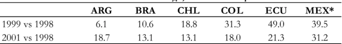
analyze the success of these policies in bringing devaluation expectations down by tracking interest rate behavior. Figure 5 shows deposit interest rates series before and after the change in regime.
The case of Colombia is a clear example of the ability of the switch in regime to reduce devaluation expectations. The expansion of the target zone in Colombia had already reduced pressure on interest rates, but the announcement of flotation with inflation targeting led to a further reduction in interest rates (from over 18 percent at the time of the announcement, to about 11 percent by end 2001). The devaluation of the exchange rate did not put excessive pressure on the fisc, nor did it apparently add excessive liabilities because of currency mismatches that could introduce uncertainty about the sustainability of monetary policy. As a result, Colombia managed to substantially reduce devaluation expectations, bringing interest rates down. However, the switch in regime was not done swiftly, and instead authorities defended the exchange rate for a long time, putting substantial pressure on interest rates. As we will see later, this could have been an important factor behind the slow recovery in economic activity.
Brazil also managed to reduce interest rates after the switch in regime, from about 35 percent at the time of the switch, to about 18 percent by end 2001, and in this respect the country regained credibility regarding its monetary regime. Still, though, interest rates have remained high in real terms. Although Brazil was not subject to large debt valuation effects at the time of the crisis, interest rates took a while before they fell. This fed into the fiscal deficit, and despite Brazil’s fiscal effort to increase its primary surplus (equivalent to 3 percentage points of GDP), debt increased substantially from 51 to 68 percent of GDP. This deterioration in sustainability may be a factor behind the interest rates’ resistance to falling further.
Figure 5. Deposit Interest Rates Behavior Argentina Brazil Chile Colombia Ecuador México 10 15 20 25 30 35 40 45 50 Jan-98 Ap r-98 Jul -98 Oct-98 Jan-99 Ap r-99 Jul -99 Oct-99 Jan-00 Ap r-00 Jul -00 Oct-00 Jan-01 Ap r-01 Jul -01 Oct-01 0 5 10 15 20 25 30 Jan-98 Ap r-98 Jul -98 Oct-98 Jan-99 Ap r-99 Jul -99 Oct-99 Jan-00 Ap r-00 Jul -00 Oct-00 Jan-01 Ap r-01 Jul -01 Oct-01 5 10 15 20 25 30 35 40 Jan-98 Ap r-98 Jul -98 Oct-98 Jan-99 Ap r-99 Jul -99 Oct-99 Jan-00 Ap r-00 Jul -00 Oct-00 Jan-01 Ap r-01 Jul -01 Oct-01 5 15 25 35 45 55 65 Jan-94 Ap r-94 Jul -94 Oct-94 Jan-95 Ap r-95 Jul -95 Oct-95 Jan-96 Ap r-96 Jul -96 Oct-96 Jan-97 Ap r-97 Jul -97 Oct-97 5 15 25 35 45 55 65 Jan-98 Mar -98 May-98 Jul -98 Se p-98 Nov-98 Jan-99 Mar -99 May-99 Jul -99 Se p-99 Nov-99 Jan-00 Mar -00 5 10 15 20 25 30 35 Jan-98 Ap r-98 Jul -98 Oct-98 Jan-99 Ap r-99 Jul -99 Oct-99 Jan-00 Ap r-00 Jul -00 Oct-00 Jan-01 Ap r-01 Jul -01 Oct-01
Note: A six-month moving average is also included. A vertical line indicates the abandonment date of prevailing exchange rate regimes. For the case of Ecuador, a second line indicates the announcement of dollarization.
Source: IMFIFS, and Central Bank of Ecuador.
Chile also managed to reduce interest rates by abandoning its previous regime. Although most of the fall in interest rates materialized after the flexibilization of the band of December 1998, there has been an additional milder fall after the adoption of the inflation-targeting regime in September 1999, with interest rates floating below 10 percent by 2001. Chile was able to accommodate to its new regime without any fiscal costs, something that contributed highly to the success of this policy.
The Mexican case is quite different in this respect. Interest rates remained high for several years before they converged to reasonable levels. Although Mexico does not seem to have been too vulnerable to valuation effects, high interest rates led to bankruptcies, which took time to be resolved, and eventually led to a bailout of the banking system estimated in nearly 20 percent of GDP. This pressure, coupled with a less clear-cut monetary policy, may be responsible for the long time it took for interest rates to converge.
Argentina managed to fight against devaluation expectations for a long time, but its fiscal stance was quickly deteriorating due to fast-rising interest payments. These, in turn, were a consequence of Argentina’s precarious sustainability position once RER realignment is factored in. Besides, expansionary monetary policy carried out in 2001, partly in an effort to recover economic activity, and partly as a consequence of the bailout of public banks facing liquidity problems, was inconsistent with a fixed exchange rate regime.21 All these events led to expectations of a balance of payments crisis, which in turn triggered a massive deposit withdrawal. The latter was not only motivated by devaluation expectations (given that most deposits were denominated in foreign currency), but also by the fact that a devaluation would lead to bankruptcies in the banking sector, given that, as previously discussed, credit mismatches were substantial (recall Table 11). This, in turn, made depositors fear that they would have to pay the brunt of the bailout, and as a result, they decided to leave the banking system. This put great pressure on interest rates, which were following an explosive path that was stopped by government intervention with the introduction of a deposit freeze, currently Argentina’s main problem yet to be solved.
Ecuador’s case is perhaps the most revealing in terms of exchange rate choices. Interest rates reached their highest point just at the time of the announcement of flotation of the currency (around 55 percent), and remained high until the announcement of dollarization was made in January 2000, when interest rates fell dramatically to levels around 11 percent (see Figure 5). Still, though, this situation was not the same for the public sector. When we take a look at the behavior of public bond spreads, we observe that they remained high despite the announcement of dollarization, and only fell substantially after a debt restructuring deal was reached with private creditors (Figure 6). These events are consistent with the fact that the resignation of monetary policy was a key condition to reach stability, since it became clear that the government
had no way of monetizing its fiscal burden. But at the same time, bond spreads gave in only when fiscal resolution was addressed.
Figure 6. 500 1,000 1,500 2,000 2,500 3,000 3,500 4,000 4,500 5,000 D ec-98 Ma r-99 Ju n-99 Se p-99 D ec-99 Ma r-00 Ju n-00 Se p-00 D ec-00 Ma r-01 Jun-01 Se p-01 De c-01
EMBI+ EMBI+ Ecuador
Sovereign Bonds “Stripped” Spreads
Source: J.P. Morgan Chase. Default →
← Dollarization
← Agreement
If the effectiveness of monetary policy is measured by the ability to keep inflation within reasonable limits, inflation targeters were successful in this respect. As shown in Table 14, inflation in all these countries was kept within limits despite strong nominal exchange rate depreciation. Why the degree of pass-through of exchange rate movements to prices was so small is still a matter of research.
Table 14.
ARG BRA CHL COL ECU MEX*
1997 0.5 6.9 6.1 18.5 30.6 9.8
1998 0.9 3.2 5.1 18.7 36.1 7.0
1999 -1.2 4.9 3.3 10.9 52.2 35.0
2000 -0.9 7.0 3.8 9.2 96.2 34.4
2001 -1.0 6.6 3.7 8.0 37.0 20.6
Source: World Economic Outlook (IMF), December 2001. */ Figures for Mexico are for the period 1993-97.
Consumer Price Index, yoy % change
As stated above, Mexico was the only country among floaters that did not adopt an inflation target. Notably also, the pass through in Mexico was much higher than that in other countries. Mexican inflation remained relatively high until 1997, when it reached 20.6 percent. In a longer horizon, however, their current monetary policy has been adequate to reduce inflation to one-digit levels in 2001 (4.5 percent).
Output Behavior
Table 15 shows the evolution of GDP growth through the sudden stop years. To some extent, the way economies recovered after the standstill in capital flows and the adoption of a particular exchange rate strategy is a valuable measure of success. Clearly, Chile is the country that best fits the main story line described in this paper. It was able to adopt an independent monetary policy, i.e., a monetary policy not subordinated to fiscal pressure, which allowed the country to recover faster than others. After an initial contraction of 1.1 percent of GDP, Chile experienced a strong recovery in 2000 (5.4 percent), and has succeeded in maintaining the growth pace in 2001. From previous analysis, we inferred that although Colombia was able to reduce devaluation expectations by accommodating the needed RER depreciation and switching to an inflation-targeting policy, it took a long time to do so. As shown above, high interest rates prevailed for a long time, bankruptcies developed, and output suffered.22 More recently, Colombia’s fiscal position has deteriorated (something that we will explore in the next section),
22 Additionally some impact could also have come from balance sheet effects of firms indebted abroad.
and concerns about sustainability may be affecting investment and output decisions. As a result, after a 4.1 percent contraction in 1999, recovery was slow (2.8 percent growth in 2000 and 1.4 percent in 2001). Brazil has also faced high interest rates recently that have put pressure on its fiscal position. Although growth reached 4.4 percent in 2000, it could not be sustained in 2001. Argentina is a clear-cut case of no output recovery within the sample period, given that expectations of RER realignment and fiscal unsustainabilty remained high, thus leading to the postponement of investment decisions. Ecuador experienced the worst fall within the sample countries. The combination of a sudden stop and a wrong exit policy (floating in a context of high liability dollarization) led to a strong contraction of economic activity that was only reversed when a more credible monetary arrangement was adopted and the fiscal stance was substantially improved. Finally, Mexico is the country in our sample with the fastest recovery. Note that this recovery takes place in a context of high domestic interest rates. Presumably, what led Mexico’s recovery was the fast switch to exports associated with NAFTA, and the fact that high domestic interest rates may have not been an important factor, since most investment included funding from abroad.
Table 15.
ARG BRA CHL COL ECU MEX*
1997 8.1 3.3 7.4 3.4 3.4 2.0
1998 3.8 0.2 3.9 0.6 0.4 4.4
1999 -3.4 0.5 -1.1 -4.1 -7.3 -6.2
2000 -0.5 4.4 5.4 2.8 2.3 5.2
2001 -2.7 1.8 3.3 1.4 5.2 6.8
Source: World Economic Outlook (IMF), December 2001. */ Figures for Mexico are for the period 1993-97.
Real Gross Domestic Product, yoy % change
6. What About Current Sustainability?
In response to the sudden stop in capital flows during the late 1990s, many countries of the region chose to float their exchange rate. As discussed above, given the low degree of liability dollarization and the relatively small impact of sharp RER adjustment on public finances, in
1998 nearly 30% of total debt of large non-financial enterprises was denominated in foreign currency. In part this also explains the need to defend the target zone and the delay in floating the exchange rate.
most cases this policy seems to have been adequate. However, the level of indebtedness and of liability dollarization has varied since then. In part the level of indebtedness has grown endogenously due to the increase in interest rates countries faced after the sudden stop while trying to defend their exchange rates.
A relevant question is how countries would react today to similar shocks, and whether the same type of policies would be fit now. To answer this question we revisit the sustainability exercise developed above. The fact that we conduct this experiment does not mean that we expect further shocks of this kind to materialize in the near future. As a matter of fact, some countries have been able to place bonds even after Argentina’s crisis, and so far, there have been no serious signs of contagion.23 Having said this, we analyze the impact on fiscal accounts of a RER adjustment that closes the current account gap, taking as initial conditions the fiscal stance and interest rates prevailing in 2001. Results are reported in Table 16.
It is important to note that the departure point of many of the countries in the sample, in terms of their debt to GDP ratio, is significantly higher than that in 1998. Brazil, for example increased its debt to GDP ratio to 68.1 (17.1 percentage points greater than in 1998) and Colombia to 49.1 (20.7 greater than in 1998). Additionally, countries like Argentina and Brazil face higher interest rates now.
The basic sustainability exercise shows important need of adjustment when we compare the required primary surplus after the depreciation to currently observed surpluses in Argentina, Brazil and Colombia. The reason that motivates this adjustment however differs between Argentina and the other two countries. The high degree of dollarization and mismatches in Argentina, coupled with a fragile fiscal position, raises concerns about the ability to conduct independent monetary policy. Indeed, fiscal dominance may be present for some time. This situation worsens when we consider the materialization of contingent liabilities. An immediate question that emerges, based on Ecuador’s experience, is whether Argentina’s recent choice to float its exchange rate and announce a monetary target was the right exchange rate strategy given its high degree of dollarization, fiscal unsustainability, and the underlying collapse of demand for domestic currency-denominated money assets.