THE CURRENT ACCOUNT AND THE NEW RULE IN A NOT-SO-SMALL OPEN ECONOMY

(1)

vol. XXXIII (3), 2009, 529-557

THE CURRENT ACCOUNT AND THE NEW RULE

IN A NOT-SO-SMALL OPEN ECONOMY

IÑAKI ERAUSKIN-IURRITA Universidad de Deusto-ESTE

This paper provides an extension of the new rule for the current account [Kraay and Ventura (2000)], abandoning the small open economy assumption: the response of transitory income shocks on the current account is equal to the new rule (savings generated by the shock multiplied by the domestic holdings of foreign assets over total domestic assets) plus the saving generated by the shock in the foreign economy multiplied by the foreign country’s share of domestic capital in foreign total assets. The extended new rule provides a good description for the behavior of current accounts, and is even better than the new rule, which would be rejected by recent evidence.

Keywords: Current account, intertemporal approach, traditional rule, new ru-le.

(JEL F41, F43)

1. Introduction

International ﬁnancial integration has accelerated enormously in re-cent years, which has implied a tremendous change in the magnitude of cross-border holdings of assets and liabilities. For example, while in the period 1970-1995 only 3.4% of the domestic capital in the USA I deeply thank Javier Gardeazabal for all his help. I also thank two anonymous re-ferees, The Co-editor Gabriel Pérez Quirós, Cruz Ángel Echevarría, Asier Minondo, Jesús Vázquez, Rafael Doménech, Antonio Fatás, José García Solanes, Salvador Or-tigueira, Philippe Bacchetta, Javier Coto-Martínez, and seminar participants at the VIII Encuentro de Economía Aplicada, at the XXIX Simposio de Análisis Econó-mico, and at the University of the Basque Country (DFAE-II) for their very helpful suggestions and comments. I am very much indebted to Jaume Ventura for kindly providing me with the data set for Kraay and Ventura (2000). The ﬁnancial support of Diputación Foral de Gipuzkoa (through the Departamento para la Innovación y la Sociedad del Conocimiento, via Red Guipuzcoana de Ciencia y Tecnología) and Gobierno Vasco (through the Programa de ayudas para apoyar las actividades de grupos de investigación del sistema universitario vasco) is gratefully acknowledged. The remaining errors and omissions are entirely the responsibility of the author.

(2)

was owned, on average, by foreign investors, in the recent period 1996-2004 this had reached 16.1%. Similar numbers apply to many countries around the world: in Germany, for instance, the percentage of domestic capital in the hands of foreign investors increased from 2.3% during 1970-1995 to 9.7% in the period 1996-2004; in Spain the increase was from 4.8% to 17.1%.1 As Lane and Milesi-Ferretti (2007, p. 224) put it, “In particular, the size of countries’ external position is now such that ﬂuctuations in exchange rates and asset prices cause very signi-ﬁcant reallocations of wealth across countries”. This has important implications for the behavior of current accounts.

According to the standard version of the intertemporal approach to the current account (or the traditional rule), the impact of transito-ry income shocks (ﬂuctuations in output, for example) on the current account is equal to the amount of saving generated by the shock in all countries since countries invest the marginal unit of wealth in for-eign assets. This occurs when investment risk is weak and diminishing returns are strong2. As is widely known, the empirical evidence is at odds with the traditional rule: “there are some patterns in the current accounts of industrial countries that are inconsistent with the basic theory that international economists have been using for more than two decades” (Ventura, 2003, p. 510). Recent studies have challenged the traditional rule [Kraay and Ventura (2000), Ventura (2001), Kraay and Ventura (2003), and Ventura (2003); K&V hereafter]. According tothe new rule,the impact of transitory income shocks on the current account is equal to the saving generated by the shock multiplied by the country’s share of foreign assets in total assets, since “the country invests the marginal unit of wealth as the average one” when invest-ment risk is strong and diminishing returns are weak (K&V, 2000, p. 1138). The new rule seems to be well supported in the long run, as well as in the short run (once costs of adjustment to investment are in-troduced) [K&V (2003); and Ventura (2003)]. However, an important implicit assumption both in the traditional rule and in the new rule is that the country is a small open economy. Thus foreign holdings of domestic capital are assumed to be constant, which is clearly re-strictive, especially when ﬁnancial markets are becoming increasingly integrated.

1

See Section 3 for more details of the database upon which these numbers are based.

2

See Obstfeld and Rogo(1995, 1996), Razin (1995), and Frenkel, Razin and Yuen (1996), for example, for excellent surveys on the intertemporal approach to the current account.

(3)

This paper suggests a straightforward extension of the new rule, aban-doning the small open economy assumption. It analyzes the impact of transitory income shocks on the current account in a two-country sto-chastic growth model. According to the extended new rule, the impact of transitory income shocks on the current account is equal to the new rule plus an additional term. This term captures the saving generated by the income shock in the foreign economy multiplied by the foreign country’s share of domestic capital in foreign total assets. The extend-ed new rule provides a good description for the empirical evidence on current accounts for 19 OECD countries in the period 1970-2004, both in the short run and the long run, and is even better than the new rule. Additionally, we have found that the new rule would be rejected by recent evidence.

2. Theory

2.1 Basic structure

The world economy is composed of two countries, each of them produc-ing only one homogeneous good. Each country has a representative agent with an inﬁnite time horizon. The homogeneous good produ-ced by both countries can be either consumed or invested in capital without having to incur in any kind of adjustment costs. There are three assets: domestic capital, foreign capital and bonds. Unstarred variables refer to the domestic economy, whereas the starred variables refer to the foreign economy. Both domestic capital, N, and foreign capital,NW_{, can be owned by the domestic representative agent or the} foreign representative agent. The subscript g denotes the holdings of assets of the domestic representative agent and the subscripti denotes the holdings of assets of the foreign representative agent. It must be satisﬁed, therefore, that

N = Ng+Ni

(4)

Domestic production is obtained using only domestic capital,N, thro-ugh an DN function, and it is expressed through a ﬁrst order stocha-stic dierential equation, so that production ﬂow g\ is subject to a stochastic disturbance

g\ =Ngw+Ng|>

where A 0 is the marginal physical product of domestic capital. The term g| represents a proportional domestic productivity shock:

g| is the increment of a stochastic process |. Those increments are temporally independent and are normally distributed. They satisfy thatH(g|) = 0andH(g|2) =2|gw.3 We omit, for convenience, formal references to time, although those variables depend on time. Note that

g\ indicates the ﬂow of production, instead of\, as is ordinarily done in stochastic calculus.

The foreign economy is structured symmetrically to the domestic eco-nomy. Thus, foreign production is carried out using capital domiciled abroad,NW_{, with a production function very similar to the one in the} domestic economy

g\W =WNWgw+NWg|W>

where W A0 is the marginal physical product of foreign capital. The term g|W _{represents a proportional foreign productivity shock and} it is the increment of a stochastic process |W. Those increments are temporally independent and are distributed normally, satisfying that

H(g|W_{) = 0} _{and that}_H(g|W2_{) =}2

|Wgw. Furthermore, shocks are

corre-lated across countries: H(g|g|W) =||Wgw.

In addition, bonds pay an instantaneous risk-free interest rate . The domestic economy can be lending to (and thus E A 0) or borrowing from (and thus E ?0) the foreign economy. Thus E denotes the net position of risk-free loans. The wealth of the domestic representative agent, Z, and the wealth of the foreign representative agent, ZW, therefore will be

Z = Ng+NgW+E [1]

ZW = Ni+NiWE= [2]

3_{That is, the production ﬂow follows a Brownian motion with drift}

N and with variance N22|.

(5)

The net foreign asset position for the domestic economy,S, is deﬁned as

S =NgWNi +E> [3]

where changes in any of those variables lead to changes in the net foreign asset position.

The current account of the domestic economy, FD, is deﬁned as the variation in its net foreign asset position given by [3], gS. Thus we have that

FD=gS =gNgWgNi +gE= [4]

This means that, for instance, the current account is positive if and only if the variation in NW

g and E is higher than the variation inNi. We can convert equation [4] into

FD=gZ gN =gZgZCNg

CZ gZ

WCNi

CZW= [5]

Thus equation [5] is the national account identity, where the current account balance is equal to the variation in domestic wealth minus the variation in domestic capital. Please note that the variation in domestic wealth, gZ, is equal to the national savings for the period,

V, that is, national income minus (private and public) consumption. Additionally, the variation in domestic capital, gN, is equal to the domestic net investment for the period.

2.2 The domestic economy

The preferences of the domestic representative agent are represented by an isoelastic intertemporal utility function where utility is obtained from consumption, F H0 Z _" 0 F1 h 3w_gw _[6] 4? ?1=

The welfare of the domestic representative agent in period 0 is the expected value of the discounted sum of instantaneous utilities, condi-tioned on the set of disposable information in period 0. The parameter

(6)

is a positive subjective discount rate (or rate of time preference). For the isoelastic utility function the Arrow-Pratt coe!cient of rela-tive risk aversion is given by the expression 1. When = 0 this function corresponds to the logarithmic utility function. The restric-tions on the utility function are necessary to ensure concavity with respect to consumption.

The domestic representative agent consumes at a deterministic rate

F(w)gw in the instantgw and thus the dynamic budget restriction can be expressed in the following way

gZ = [Ng+WNgW+E]gw+ [Ngg|+NgWg|W]Fgw= [7] If we deﬁne the following variables for the domestic representative agent

qg Ng

Z = share of the domestic portfolio materialized

in domestic capital

qW_g N

W g

in foreign capital,

qe E

in bonds,

equation [1] can be expressed more conveniently as

1 =qg+qWg+qe> [8]

and plugging [8] into the budget constraint [7] we obtain the following dynamic restriction for the resources of the domestic economy

gZ

Z =#gw+gz> [9]

where the deterministic and stochastic parts of the rate of growth of assets,gZ@Z, can be expressed in the following way

# ()qg+ (W)qWg+ F Z F Z [10] gz qgg|+qWgg|W> [11]

(7)

where qg+WqWg+qe ()qg+ (W)qWg+ denotes the gross rate of return of the asset portfolio.

The objective of the domestic representative agent is to choose the path of consumption and portfolio shares that maximizes the expected va-lue of the intertemporal utility function [6], subject to Z(0) = Z0, [9], [10], and [11]. This optimization is a stochastic optimum con-trol problem.4_{The macroeconomic equilibrium is derived in Appendix}

A1. The equilibrium (implicit) portfolio shares and the consumption-wealth ratio in the domestic open economy are given by equations [A1.9], [A1.10], [A1.11] and [A1.12] in Appendix A1,

= (1)£qg2|+qWg||W ¤ [12] W = (1)£qWg2|W+q_g||W¤ [13] qe = 1qgqWg [14] F Z = 1 1 £ + 0=5(1)2z ¤ > [15] where 2z =q2g2|+ 2qgqgW||W+qW_g22_|W=

Appendix A2 shows that second order conditions are satisﬁed. 2.3 The foreign economy

The equilibrium facing the foreign representative agent can be formu-lated in an analogous way as

= (1W)£qi2|+qWi||W¤ [16] W = (1W)£qiW2|W+q_i||W¤ [17] qW_e = 1qi qWi [18] FW ZW = 1 1W £ WWW+ 0=5W(1W)2_zW ¤ > [19] where

4_{To solve problems of stochastic optimum control see, for example, Kamien and}

Schwartz (1991, section 22), Malliaris and Brock (1982, ch. 2), Obstfeld (1992), or Turnovsky (1997, ch. 9; 2000, ch. 15).

(8)

= d ¡ 2_|W||W¢+0_d¡2_|_||W¢ 2|+2|W2||W +(1) (1W) ¡ 2_|||W¢ ¡2_|W||W¢(Z+ZW) h 2_|+2_|W2||W i [Z(1W_{) +}_ZW₍₁_)] +(W) £ Z(1W)¡2|||W ¢ 2|WZW(1) ¡ 2|W_||W ¢ 2| ¤ h 2|+2|W2||W i [Z(1W_{) +}_ZW₍₁_)] > where 0d=W(1)2|W= qW_e = E ZW 2_zW = q2_i2_|+ 2q_iqW_i_||W+qW_i22_|W=

2.4 The equilibrium interest rates

In a closed domestic economy there is no trade in any inside asset, such as a risk-free bond. In autarky the equilibrium risk-free interest rate in the domestic economy, _d, becomes, from equation [12],

d=(1)2|=

Similarly, in autarky the equilibrium risk-free interest rate in the for-eign economy,Wd, is given by equation [16]

W_d =W(1W)2_|W=

The equilibrium world risk-free interest rate in an open economy where the representative agent holds domestic capital, foreign capital, and bonds is derived by equations [12], [13], [14], [16], [17], and [18], and by the requirement that the world bond market clears, that is,

Z qe+ZWqWe = 0=

Combining those equations, the world risk-free interest rate is expres-sed as

(9)

The world risk-free interest rate is time-varying. It depends on the autarky risk free rates, on the world distribution of wealth, on the value of the parameters related to risk aversion, and so on. Since world risk-free interest rate is time-varying, portfolio shares and growth rates are also time-varying5.

2.5 The rules

Once world equilibrium has been derived the impact of transitory in-come shocks on current accounts can be discussed. For simplicity and without loss of generalization, the impact of changes in foreign hold-ings of domestic capital on domestic productivity is assumed to be negligible, _CNC

i = 0. Additionally, the impact of changes in domestic

and foreign holdings of foreign capital on foreign productivity is also assumed to be negligible, _CNCWW

g =

CW

CNW

i = 0.

A small open economy implies that foreign holdings of domestic capital are constant6:gNi = 0(See equation [4] or [5]).

Now, in case domestic capital and foreign capital are subject to dimi-nishing returns to capital in equations [12] and [16],7 then, combining equations [12] and [13], and totally dierentiating, we get that,

CNg CZ = Ng Z Z+> [20] where = " (1)2| 2||W (1)2_|W # × µ C CNg ¶31 =

Therefore, in a small open economy, if risk associated with investment is low compared to the diminishing returns eect, that is, $ 0, we get in equation [20] that CNg@CZ = 0, or expressed in another way, “in existing intertemporal models of the current account countries invest the marginal unit of wealth in foreign assets” (K&V, 2000, p. 5

See Devereux and Saito (1997). In addition to the closed economy, two scenarios are considered for the open economy and logarithmic utility in their paper: countries invest in domestic and foreign capital (and there is no bond trade in equilibrium), on the one hand, and countries invest in their own capital and bonds (but not in the capital of the other country), on the other hand.

6

See K&V (2000, p. 1145, footnote 7).

7_{Corsetti (1997), for example, develops a stochastic version of the Arrow-Romer}

model where aggregate capital stock has an external eect on labor productivity, but the representative ﬁrm faces decreasing returns to capital.

(10)

1138): the traditional rule. On the one hand, since diminishing returns are strong, investing abroad becomes more attractive. On the other hand, low risk associated with investment makes the investor willing to change portfolio composition. Then the impact of transitory income shocks on the current account, via equation [5], becomes

FD=gZ= [21]

The impact of transitory income shocks on the current account is equal to the saving generated by the shock: positive shocks generate sur-pluses in all countries.

However, in a small open economy, if investment risk is high compared to the diminishing returns eect, that is, $ 4, then equation [20] leads to

CNg

CZ =

Ng

Z> [22]

and “the country invests the marginal unit of wealth as the average one” (K&V, 2000, p. 1138): the new rule. On the one hand, since di-minishing returns are low, purchasing new capital is as attractive as existing capital. On the other hand, high risk associated with invest-ment makes portfolio composition more di!cult to change. Then the current account, via equation [5], becomes

FD=gZ µ N_gW+E Z ¶ = [23]

The response of current accounts to transitory income shocks is equal to the saving generated by the shock multiplied by the share of for-eign assets over total domestic wealth. This implies that a positive shock generates surpluses in creditor countries and deﬁcits in debtor countries in a small open economy.

In case risk associated with investment is neither low nor high compa-red to the diminishing returns eect, that is,0? ?4, then equation [20] gives us

0? CNg

CZ ?

Ng

Z=

This means that the reaction of investors will be somewhere between the traditional rule and the new rule: while the diminishing returns

(11)

eect makes investing abroad more attractive, investment risk makes investor unwilling to change portfolio composition.

Now the assumption of a small open economy is relaxed: the third term on the right hand side of equation [5] becomes crucial sincegNi need not equal 0. Additionally, combining equations [16] and [17] for the foreign economy, we ﬁnd that,

CNi

CZW =

Ni

ZW [24]

This means that the impact of transitory income shocks on the current account (see equation [5]) is given by

FD=gZ µ N_gW+E Z ¶ gZWNi ZW> [25]

if both the new rule (equation [22]) and the additional term implied by abandoning the small open economy assumption (equation [24]) apply. Therefore, the response of the current account, when a transitory in-come shock occurs, is equal to the new rule plus an additional term8. This term would capture the change in savings generated by the in-come shock in the foreign economy multiplied by foreign holdings of domestic capital over total foreign wealth. Please note that the change in domestic wealth is equal to national savings,gZ =V, as shown in Section 2.1 above.

In summary, the extended new rule nests the new rule as a special case where a small open economy is assumed, that is, when the impact of the foreign economy on the domestic economy (via foreign holdings of domestic capital) is negligible. In both cases, the country invests the marginal unit as the average one, since the risk associated with invest-ment is high compared to the diminishing returns eect. In contrast, according to the traditional rule, countries invest the marginal unit of wealth in foreign assets when investment risk is low compared to the diminishing returns eect.

8

Please note that the impact on current account is similar to that shown in Tur-novsky (1997, p. 436), except for the existence of risk-free loans now.

(12)

3. Data sources

The sample to test all the rules is composed of 19 OECD countries for the period 1970-20049: Austria, Australia, Belgium, Canada, Denmark, France, Germany, Greece, Iceland, Italy, Japan, The Netherlands, Nor-way, New Zealand, Spain, Portugal, Sweden, United Kingdom, and the United States10. Additionally some series for the world as a whole are estimated, as we shall show below. The data on GDP and gross na-tional savings for those countries (world included) are provided direct-ly by World Bank’s World Development Indicators (WBWDI). The data on current accounts and international investment positions have been obtained from the International Monetary Fund’s International Financial Statistics (IMFIFS). Additionally, as data on international investment positions are incomplete or missing for many countries be-fore 1980-1986, Lane and Milesi-Ferretti (2007) provide an excellent source of data for those years11. Domestic holdings on foreign capital,

N_gW, is measured as direct plus portfolio equity investment by domestic agents abroad, while foreign holdings of domestic capital, Ni, refers to direct plus portfolio equity investment by foreign agents in the do-mestic economy. The net lending position abroad, E, is the sum of the net position in portfolio debt investment, the net position in other investment assets (general government, banks, and others), reserve as-sets (minus gold) and the net position in ﬁnancial derivatives.

The gross domestic capital stock in current US dollars for the countries in the sample (and also for the world as a whole) is constructed using the procedure suggested by K&V (2000) in Appendix A2: gross do-mestic investment in current US dollars (from WBWDI) is cumulated assuming a depreciation rate of 4% per year, and adjusting the value of previous year’s stock using the US gross domestic investment de-ﬂator. The initial capital stock in 1970 is estimated using the average

9_{K&V (2003) and Ventura (2003) employ a similar sample, except for Finland,}

Ireland, Switzerland, and Turkey, which are not included. Constructing the data for Finland, Ireland and Switzerland produces inconsistent results to estimate foreign holdings of domestic capital due to the enormous and rapid increase of foreign investment in those countries.

1 0

Countries could be aggregated into larger blocks in order to test the behavior of current accounts for not-so-small open economies. However, the availability of data on international investment positions does not allow us to do so.

1 1

Please note that most of the data from IMFIFS, and Lane and Milesi-Ferretti (2007) coincide for recent years.

(13)

capital-output ratio over the period 1965-197512 [based on Nehru and Dareshwar (1993)13] multiplied by GDP in current US dollars (WB-WDI). The series for the foreign economy are estimated as follows: we take the values for the whole world and then the values for the domestic economy are substracted from it.

4. Empirical evidence 4.1 The traditional rule

We test the traditional rule following regression equation [21]

FDfw=d0+d1Vfw+xfw> [26] whereFDfwandVfwdenote current account balance and the amount of savings, respectively, both expressed as a share of GDP14, for country

fin periodw, andxfw is the error term for countryfin periodw. Under the null hypothesis that the traditional rule is true, then the parameter

d1 should be equal to one: an increase in savings leads to a one-to-one increase in the current account.

In their pioneer work Feldstein and Horioka (1980, p. 317) wanted to “[...] measure the extent to which a higher domestic saving rate in a country is associated with a higher rate of domestic investment.”, so that “with perfect world capital mobility, there should be no rela-tion between domestic saving and domestic investment: saving in each country responds to the worldwide opportunities for investment while 1 2

The initial value for capital-output ratio for the world is the weighted mean of capital-output ratios in the sample of 19 countries for the period 1965-1975.

1 3

Please note that the EU KLEMS Productivity Report, ﬁrst released in March 2007, provides data on economic growth, productivity, employment creation, and capital formation at the industry level for EU member states, Japan and the US from 1970 onwards (Timmeret. al.,2007). However, we have not employed that da-tabase for two main reasons. First, testing the extended new rule requires estimating capital stock for the world, which is not available in the EUKLEMS database. Se-cond, the database has been constructed in a similar manner to that in KV (2000), so that the results of this paper can be easily compared with those of previous literature.

1 4

Two dierences arise between the testing pursued by Feldstein and Horioka (1980) and by K&V(2000). First, Feldstein and Horioka regressed investment on savings. Instead, K&V regressed the current account on savings, making it easier to compare the new rule with the traditional rule. However, both approaches are equivalent. Second, Feldstein and Horioka used data related to Gross Domestic Product, whe-reas K&V used data related to Gross National Product. Here we are inclined to use GDP for the testing.

(14)

investment in that country is financed by the worldwide pool of capi-tal.” They find that the empirical evidence runs in favor of a strong relationship between both variables, thus attributing it to the lack of perfect world capital mobility. According to Frankel (1992, p. 41), “Feldstein and Horioka upset conventional wisdom in 1980 when they concluded that changes in countries’ rate of national saving had very large eects on their rates of investment and interpreted this finding as evidence of low capital mobility”. However, many economists do not share Feldstein and Horioka’s conclusion. The paradox of having perfect capital mobility alongside a strong association between savings and investment has been termed the Feldstein-Horioka puzzle. Many studies followed suit and analyzed the reasons to explain the evidence, while assuming perfect world capital mobility. However, “it seems like-ly that of many potential explanations of the Feldstein-Horioka results, no single one fully explains the behavior of all countries”, according to Obstfeld and Rogo(1995, p. 1779). We should note that Feldstein and Horioka (1980, p. 319) were aware that a high association “could reflect other common causes of the variation in both saving and in-vestment”, but they argued that a high association “would however be strong evidence against the hypothesis of perfect capital mobili-ty and would place on the defenders of that hypothesis the burden of identifying such common causal factors.” Recent empirical studies suggest that the Feldstein-Horioka finding is losing some support in the euro area (Blanchard and Giavazzi, 2002)15_.

Table 1 shows the results of ﬁtting equation [26] by ordinary least squares (OLS). The estimate falls very far from 1, thus rejecting the traditional rule, as expected. That is, of course, another piece of evi-dence in favor of the Feldstein-Horioka puzzle. Additionally, we show the between-group estimates (that is, based on the mean values of 1 5_{See Giannone and Lenza (2008) for a recent paper on the Feldstein-Horioka result.}

TABLE1

The traditional rule P

Poooolleedd rreeggrreessssiioonn BBeettwweeeenn rreeggrreessssiioonn WWiitthhiinn rreeggrreessssiioonn Gross national saving/GDP 0.3421 0.3559 0.3405

(0.0368) (0.1231) (0.1061)

R² 0.1796 0.3297 0.0929

No. of observations 608 19 608 Standard errors are in parenthesis.

Sources: IMFIFS, WBWDI, Lane and Milesi-Ferretti (2007), Nehru and Dhareshwar (1993), and own elaboration.

(15)

the variables of the group) and the within-group estimates (that is, in terms of deviations from the mean values of the variables of the group). In any case the null hypothesis that the traditional rule is true is rejected. Similar results are found in K&V (2000, 2003), and Ventura (2003).

Since other variables may inﬂuence the behavior of current accounts some control variables have been included in the regression equa-tion. They include population and output per capita (both in levels and growth rates), so that the size and development of the economy are considered; and a time trend that can capture possible upward or downward movements in economic variables. Now the period analy-zed is restricted to 1975-2004 for the same set of countries owing to data availability. When control variables are added to the regression, these variables have some eect on the dierent estimates of the co-e!cient d1, as shown in Table 2. Nonetheless, the traditional rule is again rejected by the data.

4.2 The new rule

We test the new rule with the equation [23]

FDfw=d0+d1 µ_NW g>fw+Efw Zfw ¶ Vfw+xfw= [27] TABLE2

The traditional rule (with control variables) P

Poooolleedd rreeggrreessssiioonn BBeettwweeeenn rreeggrreessssiioonn WWiitthhiinn rreeggrreessssiioonn Gross national saving/GDP 0.3481 0.2711 0.4507

(0.0325) (0.1045) (0.0809)

Time trend 0.0001 0.0008

(0.0002) (0.0015)

Population 5.64E-11 5.45E-11 -7.79E-10 (2.02E-11) (6.67E-11) (4.60E-10) Population growth -0.0254 -0.0385 -0.0119

(0.0029) (0.0096) (0.0046) GDP per capita 1.83E-06 2.17E-06 9.29E-07 (4.71E-07) (1.25E-06) (4.64E-06) GDP per capita growth -0.0025 -0.0006 -0.0025

(0.0007) (0.0100) (0.0008)

R² 0.3951 0.7518 0.2279

Sources: IFS (IMF), WDI (WB), Lane and Milesi-Ferretti (2007), Nehru and Dhareshwar (1993), and own elaboration.

(16)

Under the null hypothesis that the new rule is true, then the parameter

d₁ should be equal to one: increases in savings lead to variations in the current account that are equal to the fraction of the net foreign asset position for country fin periodwwith respect to the level of domestic wealth for country f in period w. Current account balance and the amount of savings are expressed as a share of GDP.

Table 3 reports the results of fitting equation [27] by OLS. The poo-led regression generates an estimate of d₁ equal to0=75. The between estimate is closer to 1and provides a better fit to the evidence on cur-rent accounts. However, the within estimate is slightly above0=60and the goodness-of-fit of the regression falls drastically. Including control variables in the estimation of the new rule oers estimates in the ran-ge of 0=60 and 0=70, as shown in Table 4. These results suggest that the new rule is losing support for the whole period 1970-2004. In fact, the null hypothesis that the new rule is true is rejected by the

empi-TABLE3

The new rule P

Poooolleedd rreeggrreessssiioonn BBeettwweeeenn rreeggrreessssiioonn WWiitthhiinn rreeggrreessssiioonn Gross national saving/GDP

× Net foreign assets over wealth 0.7470 0.8454 0.6315 (0.0518) (0.1562) (0.1827)

R² 0.3900 0.6327 0.2201

Sources: IMFIFS, WBWDI, Lane and Milesi-Ferretti (2007), Nehru and Dhareshwar (1993), and own elaboration. TABLE4

The new rule (with control variables) P

Time trend -0.0011 0.0005

(0.0002) (0.0014)

Population -5.03E-11 -5.05E-11 -6.05E-10 (2.24E-11) (4.82E-11) (3.96E-10) Population growth -0.0152 -0.0198 -0.0086

(0.0021) (0.0086) (0.0048) GDP per capita 2.54E-06 2.79E-06 -1.38E-06

(4.87E-07) (8.73E-06) (3.99E-06) GDP per capita growth -0.0007 0.0087 -0.0008

(0.0006) (0.0076) (0.0006)

R² 0.4793 0.8532 0.2674

(17)

rical evidence in all cases, except for the within estimate in the first regression (without control variables). Additionally, we find that the new rule explains the dynamics of current accounts in the long run much better than in the short run, as already pointed out by K&V (2003) and Ventura (2003): the new rule fits the data reasonably well in the pooled and in the between-group estimations, but “explains es-sentially none of the year-to-year within-country dierences in current accounts.” (K&V, 2003, p. 69). Let us now turn to each of these two issues.

Why has the new rule received less support in the whole period 1970-2004 than in previous estimations? Can the addition of recent data explain the dierence between more recent estimates and older esti-mates? It seems so. If we restrict testing the new rule to the period 1970-1997 (1997 is the ﬁnal period in K&V), the empirical evidence runs again in favor of the new rule, as shown in Table 5: the estimates are very close to1 (and the null hypothesis cannot be rejected, except strictly for the pooled), while some divergence between long run and short run behavior arises again.16

K&V (2003) argue that the dierences arising in the between and within estimations of the new rule have to do with the dierences in the short run and long run behavior of the current account: the new rule provides a good explanation of the long run behavior, but not so in the short run. Adjustment costs of investment are a key ele-ment explaining this divergence. Countries facing a transitory income shock modify their portfolio composition in the short run, investing most of their savings in foreign assets, when investment adjustment costs are important: portfolio rebalancing occurs. However, portfolio 1 6_{The results for the period 1970-1997 do change somewhat when control variables}

are added (not shown): the pooled and the between estimates seem to reject the new rule.

TABLE5

The new rule for the period 1970-1997 P

R² 0.3666 0.6253 0.1786

(18)

composition goes back to its initial distribution in a few years17: port-folio growth takes place. K&V (2003) estimate the dynamic behavior of the current account constructing the portfolio rebalancing compo-nent, S U. If S U =FD[(N_gW+E)@Z]·V, then the dynamic linear regression can be estimated as18

S Ufw=d0+ m X q=1 dq·S Uf>w3q+ n X q=0 eq·Vf>w3q+xfw= [28] The coe!cients estimated can be used to generate the impulse res-ponse functions of portfolio rebalancing, which captures the impact of saving on portfolio composition. Table 6 shows the results for the simple case where only 5 lags of savings are considered. The impulse response function has also been estimated: it is equal to the estimated coe!cients on current and lagged saving in this case. The results imply that, when the impact occurs, the fraction of an increase in saving that countries invest into foreign assets is 0=35 (when initial foreign assets are zero). However, they gradually rebalance their portfolio composi-tion toward the initial distribucomposi-tion: the coe!cients of lags of saving in the next 5 years are negative and decreasing (in absolute terms). Those coe!cients denote the fraction of the initial increase in saving that is allocated in domestic assets again in each of the next 5 years. In fact, the sum of all the coe!cients is0=01. This would mean that the initial response toward foreign assets is reversed back to the initial composition. Results do change when lagged values of the portfolio rebalancing term are introduced, as Table 7 shows. Nonetheless, the impulse response function is qualitatively broadly similar to that re-ported in Table 6. To summarize, even though the new rule would be rejected by the recent evidence, we still ﬁnd strong support for it both in the short run and the long run.

1 7

See K&V (2003) for a formal model of current account when adjustment costs of investment are important.

1 8

Please note that current account balance and savings are expressed as a share of GDP. Standard control variables can also be included in the regression.

(19)

4.3 The extended new rule

Now the implications of abandoning the small open economy assump-tion on current accounts can be empirically estimated. The extended new rule, shown in equation [25], can be tested with the regression equation19 FDfw=d0+d1 µ_NW g>fw+Efw Zfw ¶ Vfw+d2 µ Ni>fw ZW fw ¶ VfwW +xfw= [29] Under the null hypothesis that the extended new rule is true, thend1 should be equal to 1, and d2 should be equal to 1: the impact of transitory income shocks on current accounts is equal to the saving generated by the income shock in the domestic economy multiplied by the share of domestic holdings of foreign assets over domestic wealth 1 9

All the variables are expressed as a share of GDP, as usual. TABLE6

The new rule: The short run and the long run R

Reeggrreessssiioonn IImmppuullssee rreesspp.. ffuunncctt.. C

Cooeeffff.. eessttiimmaatteess CCooeeffff.. S..ESE.. YYeeaarr IImmppuullssee rreesspp..

Sc,t 0.3484 0.0876 t 0.3484 Sc,t-1 -0.0614 0.1193 t-1 -0.0614 Sc,t-2 -0.1537 0.1177 t-2 -0.1537 Sc,t-3 -0.1456 0.1121 t-3 -0.1456 Sc,t-4 -0.0527 0.1107 t-4 -0.0527 Sc,t-5 0.0091 0.0794 t-5 0.0091 Sources: IMFIFS, WBWDI, Lane and Milesi-Ferretti (2007), Nehru and Dhareshwar (1993), and own elaboration.

TABLE7

The new rule, with portfolio rebalancing lags: The short run and the long run

R

Cooeeffff.. eessttiimmaatteess CCooeeffff.. S..ESE.. YYeeaarr IImmppuullssee rreesspp..

Sc,t 0.4058 0.0574 t 0.4058 Sc,t-1 -0.4632 0.0827 t-1 -0.3051 Sc,t-2 -0.0334 0.0837 t-2 -0.1643 Sc,t-3 0.0088 0.0764 t-3 -0.1447 Sc,t-4 0.0707 0.0693 t-4 -0.1119 Sc,t-5 0.0152 0.0499 t-5 -0.0428 PRc,t-1 0.9342 0.0432 t-6 -0.0150 PRc,t-2 -0.1707 0.0568 t-7 -0.0030 PRc,t-3 0.0466 0.0431 t-8 0.0008 Sources: IMFIFS, WBWDI, Lane and Milesi-Ferretti (2007), Nehru and Dhareshwar (1993), and own elaboration.

(20)

plus the saving generated by the income shock in the foreign economy multiplied by the share of domestic capital in the foreign economy over foreign wealth.

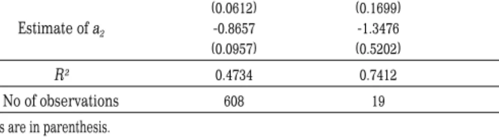
Table 8 shows the results. The pooling estimates have the expected signs and are close to their expected values: d1 is equal to1=05and d2 is equal to 0=87. The within estimates follow similar patterns (1=02 ford₁and0=74ford₂), except for the second parameter, which moves away from its expected value, even though it cannot rejected by the data. The between estimate for d1 is equal to 1=11, and that ford2 is equal to1=35: the distance from expected values widens. Nonetheless the null cannot be rejected. The evidence suggests that the extended new rule explains the evidence on current accounts better than other

TABLE8

The extended new rule P

Poooolleedd BBeettwweeeenn--ggrroouupp WWiitthhiinn--ggrroouupp rreeggrreessssiioonn rreeggrreessssiioonn rreeggrreessssiioonn Estimate of a1 1.0450 1.1121 1.0156 (0.0612) (0.1699) (0.2907) Estimate of a2 -0.8657 -1.3476 -0.7397 (0.0957) (0.5202) (0.4050) R² 0.4734 0.7412 0.2841 No of observations 608 19 608 Standard errors are in parenthesis.

Sources: IMFIFS, WBWDI, Lane and Milesi-Ferretti (2007), Nehru and Dhareshwar (1993), and own elaboration. TABLE9

The extended new rule (with control variables) P

Poooolleedd rreeggrreessssiioonn BBeettwweeeenn rreeggrreessssiioonn WWiitthhiinn rreeggrreessssiioonn Estimate of a1 0.9856 1.0718 1.2300

(0.0726) (0.2192) (0.2152) Estimate of a2 -1.1324 -1.6177 -1.3135 (0.1595) (0.6456) (0.4231)

Time trend 4.15E-05 0.0027

(0.0002) (0.0009)

Population -1.03E-10 -1.32E-10 -4.05E-10 (2.07E-11) (5.21E-11) (2.70E-10) Population growth -0.0072 -0.0056 -0.0031

(0.0021) (0.0092) (0.0039) GDP per capita 2.08E-06 3.03E-06 -4.48E-06

(4.36E-07) (7.42E-07) (2.67E-06) GDP per capita growth -0.0003 -0.0073 -1.36E-06 (0.0005) (0.0090) (0.0005)

R² 0.5498 0.9036 0.3627

(21)

rules. Similar evidence was found by Erauskin-Iurrita (2004) for the period 1973-1995. Since the goodness-of-ﬁt for the within regression is considerably lower than that of the between regression, it seems that the extended new rule explains long run behavior more satisfactorily than short run dynamics, as in the new rule. We turn to this issue below. Once the regression equation is controlled by some variables, the results for the parameterd1 remain more or less intact, as Table 9 shows. However, the estimates ford₂ become more negative and they move away from their expected values. The null cannot be rejected though.

As we mentioned before, dierences in the goodness of ﬁt for the within and between estimates suggest that the extended new rule provides a better account of long run behavior than that in the short run. Thus we are inclined to reformulate the portfolio rebalancing behavior, as above with the new rule, to take into account the extended new rule. The new portfolio rebalancing component, is denoted byS U0. If

S U0 =FD[(N_gW+E)@Z]·V+ (Ni@ZW)·VW, then the new dynamic linear regression (see equation [28]) can be estimated as20

S Ufw0 =d0+ m X q=1 dq·S U0f>w3q+ n X q=0 eq·Vf>w3q+xfw=

Table 10 shows the results for the simple case where only 5 lags of sa-vings are introduced. Countries, on impact, invest 0=48 of an increase in saving into foreign assets (for zero initial foreign assets), but then portfolio composition rebalances toward the initial composition. The coe!cients of lags of saving in the next 5 years are negative and de-creasing (in absolute terms) and the sum of all the coe!cients is equal to0=003. When lagged values of the portfolio rebalancing component are included (see Table 11) then we ﬁnd that, even though the re-sults change, they are similar, in qualitative terms, to the simple case. Therefore, the results for the extended new rule provide a good por-trayal of the evidence of current accounts, even better than the new rule, both in the short run and the long run.

2 0

Please note that current account balance and savings are expressed in terms of GDP. Control variables can also be included in the regression equation.

(22)

5. Conclusions

International ﬁnancial integration has increased tremendously in re-cent years. The subsequent dramatic growth of cross-border holdings of assets and liabilities has important implications for the behavior of current accounts since a crucial implicit assumption in models of current accounts is that the country is a small open economy. This assumption implies that foreign holdings of domestic capital are con-stant, which is very restrictive, especially when ﬁnancial markets are increasingly integrated.

According to the standard intertemporal approach to the current ac-count, or the traditional rule, the impact of a transitory income shock on the current account is equal to the savings generated by the shock one-to-one in all countries since risk associated with investment is low compared to the diminishing returns eect. The empirical evidence re-jects the traditional rule. Recent research by K&V has proposed the

TABLE10

The extended new rule: The short run and the long run R

Cooeeffff.. eessttiimmaatteess CCooeeffff.. S..ESE.. YYeeaarr IImmppuullssee rreesspp.. b0(Sc,t) 0.4754 0.0735 t 0.4754 b1(Sc,t-1) -0.0684 0.0999 t-1 -0.0684 b2(Sc,t-2) -0.1061 0.0986 t-2 -0.1061 b3(Sc,t-3) -0.1499 0.0939 t-3 -0.1499 b4(Sc,t-4) -0.0391 0.0927 t-4 -0.0391 b5(Sc,t-5) -0.1091 0.0665 t-5 -0.1091 Sources: IMFIFS, WBWDI, Lane and Milesi-Ferretti (2007), Nehru and Dhareshwar (1993), and own elaboration.

TABLE11

The extended new rule, with portfolio rebalancing lags: The short run and the long run

R

Cooeeffff.. eessttiimmaatteess CCooeeffff.. S..ESE.. YYeeaarr IImmppuullssee rreesspp.. b0(Sc,t) 0.4629 0.0541 t 0.4629 b1(Sc,t-1) -0.4541 0.0779 t-1 -0.2619 b2(Sc,t-2) -0.0327 0.0789 t-2 -0.1383 b3(Sc,t-3) 0.0013 0.0721 t-3 -0.1318 b4(Sc,t-4) 0.0598 0.0651 t-4 -0.1065 b5(Sc,t-5) 0.0349 0.0474 t-5 -0.0410 a1(PR’c,t-1) 0.8371 0.0428 t-6 -0.0147 a2(PR’c,t-2) -0.1323 0.0541 t-7 -0.0031 a3(PR’c,t-3) 0.0004 0.0419 t-8 0.0006 Sources: IMFIFS, WBWDI, Lane and Milesi-Ferretti (2007), Nehru and Dhareshwar (1993), and own elaboration.

(23)

new rule: the impact of a transitory income shock on the current ac-count is equal to the savings generated by the shock multiplied by the domestic holdings of foreign assets over total domestic assets when in-vestment risk is high compared to the diminishing returns eect. The empirical evidence supports the new rule in the long run as well as in the short run (once adjustment costs of investment are included). This paper has suggested an extension of the new rule abandoning the small open economy assumption. According to the extended new rule, the impact of a transitory income shock on the current account is equal to the response suggested by the new rule plus an additional term. This term would capture the saving generated by the shock in the foreign economy multiplied by the foreign country’s share of domestic capital in foreign total assets. We ﬁnd in this paper that the traditional rule has been unsurprisingly rejected by the empirical evidence. Nonethe-less, in contrast to recent favorable evidence, the new rule appears to be losing support: it has even been rejected by the data. However, the empirical evidence provides strong support for the extended new rule, both in the long run and the short run. Further research extending the number of countries and years involved will probably show how robust the extended new rule remains in comparison with other alternatives.

Appendixes A1. Optimization

The ﬁrst step in order to solve the optimization problem in the domes-tic economy is to introduce a value function, Y(Z), which is deﬁned as Y(Z) = P d{ {F>qg>qWg} H0 Z " 0 F₁ h 3w_gw> _[A1.1]

subject to the restrictions [9], [10], and [11] and given initial wealth. The value function in period 0 is the expected value of the discoun-ted sum of instantaneous utilities, evaluadiscoun-ted along the optimal path, starting in period 0 in the stateZ(0) =Z0.

Starting from equation [A1.1] the value function must satisfy the fol-lowing equation, known as the Hamilton-Jacobi-Bellman equation of stochastic control theory or, for short, the Bellman equation

(24)

Y(Z) = Pd{ {F>qg>qWg} · F₁ +Y 0_(Z_{)Z #}_{+ 0=5Y}00_(Z)Z22 z ¸ = [A1.2] The right hand side of equation [A1.2] is partially dierentiated with respect to F, qg and qW_g in order to get the ﬁrst order optimality conditions of this problem

F31Y0(Z) = 0 [A1.3]

Y0(Z)Z()gw+Y00(Z)Z2fry(gz> g|) = 0 [A1.4]

Y0(Z)Z(W)gw+Y00(Z)Z2fry(gz> g|W) = 0= [A1.5] The solution to this problem is obtained through trial and error. We seek a value function Y(Z) that satisﬁes, on the one hand, the ﬁrst order optimality conditions and, on the other, the Bellman equation. In the case of isoelastic utility functions the value function has the same form of the utility function [Merton (1969), then generalized in Merton (1971)]. Thus, we postulate that the value function is of the form

Y(Z) =DZ>

where the coe!cient D has to be determined. This function implies that

Y0(Z) = DZ31

Y00(Z) = D(1)Z32=

Substituting these expressions in the ﬁrst order optimality conditions [A1.3], [A1.4] and [A1.5] we derive

F31 = DZ31 [A1.6]

()gw = (1)fry(gz> g|) [A1.7]

(W₎_gw _{= (1}₎_fry_{(gz> g|}W₎₌ _[A1.8] These are typical equations in stochastic models in continuous time. Equation [A1.6] indicates that at the optimum, the marginal utility

(25)

derived from consumption must be equal to the marginal change in the value function or the marginal utility of wealth. Equations [A1.7] and [A1.8] show that the optimal choice of portfolio shares of the domestic representative agent must be such that the risk-adjusted rates of return of assets are equalized.

Combining equations [8], [A1.6], [A1.7], and [A1.8] and inserting them in the equation [A1.2], we can calculate the equilibrium portfolio shares (implicitly) and the consumption-wealth ratio in the domestic open economy = (1)£qg2|+qWg||W ¤ [A1.9] W = (1)£qWg2|W+q_g_||W¤ [A1.10] qe = 1qgqWg [A1.11] F Z = 1 1 £ + 0=5(1)2z ¤ > [A1.12] where 2z =q2g2|+ 2qgqgW||W+qW_g22_|W=

A2. Second order conditions

In this appendix we check the second order condition and the trans-versality condition.

To guarantee that consumption is positive in the domestic open econo-my we impose the feasibility condition that the marginal propensity to consume out of wealth must be positive since wealth does not become negative

1

£

+ 0=5(1)2_z¤A0=

For the ﬁrst order optimality conditions to characterize a maximum, the corresponding second order condition must be satisﬁed, that is, the Hessian matrix associated to the maximization problem and evaluated at the optimal values of the choice variables

"

(1) (Y0(Z))3312 0

0 Y00(Z)Z2

(26)

must be negative deﬁnite,21 which implies that

(1)¡Y0(Z)¢3231 _? ₀

Y00(Z)Z2 ? 0>

where=2|+ 2||W+2_|WA0. To evaluate those conditions ﬁrst we

obtain the value of the coe!cient D in equation [A1.6]

D= 1 µ F Z ¶31 > [A2.1]

where F@Z is the optimal value obtained in equation [A1.12]. Then substituting expression [A2.1] into the value function [A1.1], we get that the value function is given by

Y(Z) = 1 µ F Z ¶31 Z> [A2.2]

where we can observe that, given the restrictions on the utility functi-on, Y0(Z)A0 and Y00(Z)?0provided that F@Z A0.

In addition, we impose that the macroeconomic equilibrium must sa-tisfy the transversality condition so as to guarantee the convergence of the value function

lim w<"H h Y (Z)h3w i = 0= [A2.3]

Now it can be shown that should the feasibility condition be satisﬁed then that is equivalent to satisfying the transversality condition.22 To evaluate [A2.3], we start expressing the dynamics of the accumulation of wealth

gZ =#Z gw+Z gz= [A2.4]

The solution to equation [A2.4], starting from the initial wealthZ(0), is23

Z(w) =Z(0)h(#30=52z)w+z(w)3z(0)₌

2 1

See Chiang (1984, pp. 320-323), for example.

2 2_{See Merton (1969). Turnovsky (2000) provides, for example, the proof of the}

transversality condition as well.

(27)

Since the increments ofzare temporally independent and are normally distributed then24

H[DZ_h3w_{] =} _H[DZ₍₀₎_h(#30=52_z)w+[z(w)3z(0)]3w_]

= DZ(0)(1+)h[(#30=52z)+0=522z3]w₌

The transversality condition [A2.3] will be satisﬁed if and only if

£#0=5(1)2z

¤

?0=

Now substituting equations [10] and [A1.12], it can be shown that this condition is equivalent to

F

Z A0> [A2.5]

and thus feasibility guarantees convergence as well.

References

Blanchard, O.J., and F. Giavazzi (2002): “Current account deﬁcits in the euro area: the end of the Feldstein-Horioka puzzle?”,Brookings Papers on Economic Activity2, pp. 147-209.

Chiang, A. C. (1984),Fundamental methods of mathematical economics.Third Ed., McGraw-Hill, Singapore.

Corsetti, G. (1997): “A portfolio approach to endogenous growth: equilibrium and optimal policy”,Journal of Economic Dynamics and Control21, pp. 1627-1644.

Devereux, M. B. and M. Saito (1997): “Growth and risk-sharing with incom-plete international assets markets”, Journal of International Economics 42, pp. 453-481.

Erauskin-Iurrita, I. (2004), Three essays on growth and the world economy Unpublished PhD dissertation. University of the Basque Country, Bilbao, Spain.

Feldstein, M. and C. Horioka (1980): “Domestic savings and international capital ﬂows”,Economic Journal90, pp. 314-329.

(28)

Frankel, J.A. (1992), On exchange ratesMIT Press, Cambridge, Massachu-setts, United States of America.

Frenkel, J.A., and A. Razin, with the collaboration of Chi-Wa Yuen (1996), Fiscal policies and growth in the world economy. Third editionMIT Press, Cambridge, Massachusetts, United States of America.

Giannone, D., and M. Lenza (2008): “The Feldstein-Horioka fact”, European Central Bank, Frankfurt, working paper series, no _{873, available from}

http://www.ecb.int/pub/pdf/scpwps/ecbwp873.pdf.

International Monetary Fund (2008),International Financial Statistics. Kamien, M.I., and N.L. Schwartz (1991),Dynamic optimization. Second

edi-tionNorth-Holland, United States of America.

Kraay, A., and J. Ventura (2000): “Current accounts in debtor and creditor countries”,Quarterly Journal of Economics115, pp. 1137-1166.

Kraay, A., and J. Ventura (2003): “Current accounts in the long and the short run”,NBER Macroeconomics Annual,pp. 65-94.

Kraay, A., N. Loayza, L. Servén, and J. Ventura (2005): “Country portfolios”, Journal of the European Economic Association3, pp. 914-945.

Lane, P.R., and G.M. Milesi-Ferretti (2007): “The external wealth of nations mark II: Revised and extended estimates of foreign assets and liabilities, 1970-2004”, Journal of International Economics 73, pp. 223-250. Data available from http://www.philiplane.org/papers.html.

Malliaris, A.G., and W.A. Brock (1982), Stochastic methods in economics and ﬁnanceNorth-Holland, Amsterdam, The Netherlands.

Merton, R.C. (1969): “Lifetime portfolio selection under uncertainty: the continuous-time case”, Review of Economics and Statistics 51, pp. 247-257. Reimpressed in Merton, R.C. (1992).Continuous-time ﬁnance, Black-well, Massachusetts, United States of America.

Merton, R.C. (1971): “Optimum consumption and portfolio rules in a continu-ous-time model”,Journal of Economic Theory3, pp. 373-413. Reimpres-sed in Merton, R.C. (1992).Continuous-time ﬁnance,Blackwell, Massa-chusetts, United States of America.

Nehru, V.; and A. Dhareshwar (1993): “A new database on physical capital stock: sources, methodology and results”,Revista de Análisis Económico 8, pp. 37-59.

Obstfeld, M. (1992): “Dynamic optimization in continuous-time economic models (a guide for the perplexed)”, Working paper, available from http://elsa.berkeley. edu/ obstfeld/.

Obstfeld, M. and K. Rogo(1995): “The intertemporal approach to the cur-rent account”, In Grossman, G.M., and K. Rogo (Eds.). Handbook of international economics. Volume III.Elsevier Science B.V., Amsterdam, Netherlands.

Obstfeld, M. and K. Rogo(1996),Foundations of international macroeco-nomicsMIT Press, Cambridge, Massachusetts, United States of America. Razin, A. (1995): “The dynamic-optimizing approach to the current account: theory and evidence”, In Kenen, P.B. (Ed.).Understanding interdepen-dence. The macroeconomics of the open economy. Princeton University Press, Princeton, New Jersey, United States of America.

(29)

Timmer, M., M. O´Mahony and B. van Ark (2007),The EU KLEMS Growth and Productivity Accounts: an overview(March 2007). University of Gro-ningen and University of Birmingham; downloadable at www.euklems.net. Turnovsky, S.J. (1997),International macroeconomic dynamics MIT Press,

Cambridge, Massachusetts, United States of America.

Turnovsky, S.J. (2000),Methods of macroeconomic dynamics. Second edition MIT Press, Cambridge, Massachusetts, United States of America. Ventura, J. (2001): “A portfolio view of the US current account deﬁcit”,

Brookings Papers on Economic Activity1, pp. 241-253.

Ventura, J. (2003): “Towards a theory of current accounts”,The World Eco-nomy26, pp. 483-512.

World Bank (2007),World Development Indicators.

Resumen

Este artículo ofrece una extensión de la regla nueva para la cuenta corrien-te [Kraay y Ventura (2000)] abandonando el supuesto de una pequeña econo-mía abierta: la respuesta de los shocks de renta transitorios sobre la cuenta corriente es igual a la regla nueva (ahorro originado por el shock multiplicado por las tenencias de activos extranjeros sobre el total de los activos internos) más el ahorro originado por el shock en la economía extranjera multiplica-do por la participación que supone el capital multiplica-doméstico en el país extranjero respecto al total de activos extranjeros. La regla nueva ampliada proporciona una descripción satisfactoria del comportamiento de las cuentas corrientes, incluso mejor que la regla nueva, que sería rechazada por la evidencia recien-te.

Palabras clave: Cuenta corriente, enfoque intertemporal, regla tradicional, nueva regla.

Recepción del original, julio de 2007 Versión final, junio de 2009