A Computer Program for Flow-Log Analysis of Single Holes (FLASH)

A Computer Program for Flow-Log Analysis of Single

Holes (FLASH)

Frederick D. Day-Lewis1_{, Carole D. Johnson}2_{, Frederick L. Paillet}3_{, and Keith J. Halford}4

Abstract

A new computer program, FLASH (Flow-Log Analysis of Single Holes), is presented for analysis of borehole vertical flow logs. The code is based on an analytical solution for steady-state layer radial flow to a borehole. The code includes options for (1) discrete fractures and (2) multi-layer aquifers. Given vertical flow profiles collected under both ambient and stressed (pumping or injection) conditions, the user can estimate fracture (or layer) transmissivities and far-field hydraulic heads. FLASH is coded in Microsoft Excel5 with Visual Basic for Applications routines. The code supports manual and automated model calibration.

Introduction

Flowmeters provide means to infer the flow into or out of boreholes connected to transmissive aquifer units or fractures. In the past, the relative inaccuracy and difficult operating procedures for spinner flowmeters limited the use of borehole flow measurements. With the advent of heat-pulse (e.g., Paillet et al., 1996) and electromagnetic (Molz et al, 1994) instruments, measurements of vertical flow as small as 0.05 liters/minute became practicable, and borehole flowmeter logging is becoming routine. New modeling and analysis tools are needed to achieve the full potential of these measurements.

Calibration of a borehole flow model to flowmeter data can produce estimates of transmissivity and heads for one or more flow zones (aquifer layers or fractures). Here, we briefly review approaches for analysis of flowmeter logs and introduce a new computer program which supports manual and automated calibration of an analytical borehole flow model.

Approach

Single-hole flowmeter data can be analyzed to estimate transmissivity profiles along boreholes and characterize aquifer compartmentalization (e.g., Molz et al., 1989; Kabala, 1994; Paillet, 1998). Analysis of single-hole flowmeter data is commonly based on the Thiem Equation (Thiem, 1906), which written for confined radial flow from a single flow zone (i.e., aquifer layer or fracture) to a screened or open well is:

1 _{Corresponding Author: U.S. Geological Survey, Office of Groundwater, Branch of Geophysics, 11 Sherman Place, Unit} 5015, Storrs CT 06269; [email protected]; Phone: 860.487.7402 x21; Fax: 860.487.8802

2 _{U.S. Geological Survey, Office of Groundwater, Branch of Geophysics, 11 Sherman Place, Unit 5015, Storrs CT 06269} 3 _{U.S. Geological Survey, Emeritus, Office of Groundwater, Branch of Geophysics, 11 Sherman Place, Unit 5015, Storrs CT} 06269

4 _{U.S. Geological Survey, Nevada Water Science Center, 2730 N. Deer Run Rd., Carson City, Nevada, 89703}

5 _{Any use of trade, product, or firm names is for descriptive purposes only and does not imply endorsement by the U.S.} Government.

Final copy as submitted to Ground Water for publication as: Day-Lewis, F.D., Johnson, C. D., Paillet, F.L., and Halford, K.J., 2011, A computer program for flow-log analysis of single holes (FLASH): Ground Water, doi: 10.1111/j.1745-6584.2011.00798.x

(1)

where, Qi is the volumetric flow into the well from flow zone i [L3T-1]; hwand hi are, respectively, the

hydraulic head [L] at the radius of the well rw, and at radial distance r0, commonly taken as the radius of

influence, where heads do not change as a result of pumping, in which case hi is the connected far-field

head for zone i; and Ti is transmissivity of flow zone i [L2T-1].

A number of approaches to flowmeter analysis have been proposed and demonstrated for different sets of assumptions (e.g., no ambient flow in boreholes) and data requirements (e.g., flow profiles collected under both ambient and stressed conditions) based either on Equation (1) (e.g., Molz et al., 1989) or quasi-steady flow approximations (e.g., Paillet, 1998). We refer the interested reader to Williams et al. (2008) for additional background on flowmeter logs and focus the following discussion on the approach of Paillet (1998, 2001) which is adapted here.

Paillet (1998) formulated flowmeter log analysis as a model calibration procedure involving flow profiles collected under both ambient and stressed (pumping or injection) conditions.

Consideration of the two conditions allows for estimation of the transmissivities and also far-field heads of flow zones. The latter is critical for interpretation of water samples from wells that intersect multiple fractures or layers with different hydraulic head (e.g., Johnson et al., 2005). Applying Equation (1) to an ambient condition (condition a) and a stressed condition (condition s) gives:

















where, is the fraction of the borehole’s transmissivity contributed by flow zone i [-]; is the total transmissivity of the flow zones intersected by the borehole [L2T-1]; , are the ambient and stressed water levels in the well, respectively [L]; is the far-field head in flow zone i [L];

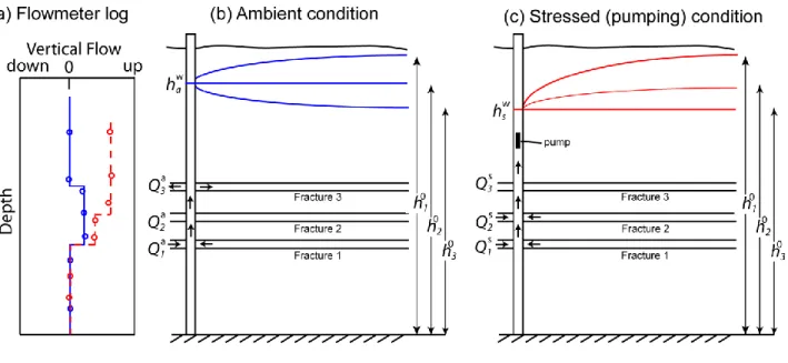
For both ambient and stressed conditions, the water level in the borehole is assumed to be constant in time, and the water level in the far field of each zone is assumed to be the natural condition, i.e., . In a field experiment (Fig. 1), rw would be known, and the flow rates and water levels in the

well would be measured. Radius of influence can be inferred experimentally based on head data at observation wells, in which case r0 can be constrained during calibration, or else it can be approximated

(e.g., Bear, 1979, p. 306). Estimates of transmissivity are not strongly sensitive to the value assumed for

r0 because it appears inside the logarithm in Equations (2-3). For example, a change in r r0 w from 10 to

100 yields a change in the estimated Ti of only a factor of 2, and order-of-magnitude estimates of

transmissivity are acceptable for many problems. In cases where knowledge of r0 is unavailable, but the

borehole’s total transmissivity is known from specific-capacity or slug-test results, it is possible to estimate r0 in the calibration procedure. We note that the forward model (Equations 2, 3) produces twice

as many independent equations as there are flow zones, with an additional equation requiring values to sum to 1. The number of parameters being estimated is twice the number of flow zones

( ) plus one parameter for either or .

Model calibration involves changing the model parameters such that the flows predicted by Equations (2-3) match the interpreted flow profiles. Following Paillet (1998, 2001), calibration is to the interpreted profile and not individual data. This formulation allows the user to incorporate additional

insight (e.g., from other logs) to identify the number and locations of flow zones and eliminates the need for weighting measurements differently according to variable measurement errors and the spatial

distribution of measurements along the borehole.

Calibration can be implemented by manual trial-and-error or automated using nonlinear regression. Whether manual or automated, the goal for calibration is to identify the set of parameters that minimize a measure of combined data misfit and model misfit. Consideration of model misfit criteria, commonly referred to as regularization, is useful when multiple models can match the data equally well or within measurement errors. Here, the data misfit is formulated based on squared differences between the predicted and interpreted flow profiles, such that multiple measurements may be collected in a single borehole interval. The model misfit could be formulated in different ways, but we use criteria based on the differences between the water level in the borehole under ambient

conditions and the far-field heads. Thus, the objective function, F, consists of two terms: (1) the mean squared error (MSE) between interpreted and predicted flow profiles, with equal weights for all cumulative flows (ambient and stressed), and (2) the sum of squared differences ( ) between the borehole's water level and far-field heads:

(4) subject to constraints

where, Q_ia int, ,Q_is int, are the interpreted flow profiles (i.e., cumulative flow above zones) for zone i under ambient and stressed conditions, respectively [L3T-1]; Q_ia sim, ,Q_is sim, are the simulated flow profiles (i.e., cumulative flow above zones) for zone i under ambient and stressed conditions, respectively [L3T-1]; α weights the regularization relative to the data misfit [L4T-2]; T_minfactor is the user-specified minimum Tfactor

for any flow zone which can ensure non-negative Tfactor; is the user-specified maximum

absolute difference between the ambient water level and the far-field head of any flow zone; and n is the number of flow zones.

Without regularization, F reduces to the MSE between simulated and interpreted flows. The tradeoff parameter  is set by the user, with larger values more strongly penalizing large head

differences. Commonly, small values (<0.001) are sufficient to obtain good results. In selecting , the user should be guided by the goal of regularization, which is to identify the "simplest" explanation of the data while minimizing the data misfit.

Using Flash

FLASH (Flow-Log Analysis of Single Holes) is written in Excel with Visual Basic for Applications (VBA). The spreadsheet includes a toggle (INPUTS worksheet cell A20) to choose between analysis for (1) fractures or fracture zones that intersect a well at discrete locations, and (2) aquifer layers in porous media. The first is indicated for cases where flow profiles are characterized by step increases/decreases, and the second for cases where flow profiles show approximately linear change over each layer. Up to 10 fractures or layers can be modeled.

The FLASH spreadsheet includes four worksheets: INTRODUCTION, INPUTS,

FIELD_DATA, and PLOTTING. INTRODUCTION provides information about the program and input parameters. On the INPUTS worksheet, the user enters information about the flow zones,

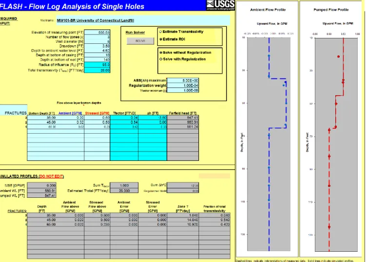
both the ambient and stressed conditions. The flow measurements are entered in FIELD_DATA, and the interpreted profiles are entered in INPUTS. The interpreted profiles plot as dashed lines, the data as points, and the simulated profiles as solid lines (Figure 2). Line and marker styles can be modified using standard Excel tools. Flows are positive upward and negative downward. PLOTTING is used by the program and does not require the user's attention.

In the INPUTS worksheet, input parameters are entered in the cells with light blue and bright aquamarine backgrounds. The former include specifications of the experiment setup (e.g., borehole diameter and water level), and the latter include calibration parameters. Manual calibration is performed by adjusting the values of the cells ―TFactor‖ and “h,” which are, respectively, factor

i

T , and the difference between the flow zone’s far-field head and the ambient water level in the borehole. As parameters are adjusted, the simulated flow profiles update automatically, thus guiding the user toward best-fit parameters. The MSE between simulated and observed flows is calculated in cell B36 on the INPUTS worksheet.

Although the principle calibration parameters are T_ifactor and h, the radius of influence, r0, and

total transmissivity, Ttotal, also are possible calibration parameters as explained above and indicated by aquamarine highlighting. By inspection of Equations (2-3), it is not possible to estimate unique values for both radius of influence and total transmissivity, but only the ratio of total transmissivity divided by ln(r0/rw). In general, the user will have more information about total transmissivity than radius of

influence. Total transmissivity is estimated readily using an open-hole slug test or specific capacity test. Indeed, the drawdown and pumping rate under stressed conditions could serve as data to estimate a total transmissivity for the borehole. In rare cases, however, the estimated total transmissivity may be

considered unreliable, e.g., in the presence of ambiguous slug-test data or discrepancy between the volumes over which the slug test and flowmeter analysis measure. In such cases it may be useful to allow theTfactorvalues to sum to a value other than 1. FLASH assumes a uniform radius of influence for all flow zones. In reality the effective radius of influence may vary between zones according to their transmissivities and distances to boundaries. Data to support variable radius of influence, however, is commonly unavailable; furthermore, transmissivity estimates are not a strong function of the assumed radius of influence, as explained previously.

Automated model calibration is implemented using the Excel Solver, an optimization tool based on a Generalized Reduced Gradient algorithm (Lasdon and Smith, 1992). The Solver is invoked using VBA ―control buttons‖ on the INPUTS worksheet. Radio buttons allow for selections of (1) the parameters to be estimated (Estimate ROI (radius of influence) or Estimate Transmissivity), and (2) regularization (Solve without Regularization or Solve with Regularization). Under the option Estimate ROI, the Solver estimates the values of T_ifactorfor all i, and the single radius of influence. Under the option Estimate Transmissivity, radius of influence is assumed known, the parameters for estimation are

factor i

T for all i, such that total transmissivity is allowed to vary. Users are encouraged to perform manual calibration before attempting automated calibration. Manual calibration provides insight into the

sensitivity of flows to parameters, and helps to identify a good starting model for automated calibration. As for any non-linear optimization, the algorithm may get ―stuck‖ in local minima and fail to identify the globally optimal parameter values. Consideration of multiple starting models is advised. Additional information and the FLASH spreadsheet are available online, as noted under 'Supporting Information' at the end of this article.

Example

FLASH is demonstrated for a simple dataset from a fractured-rock aquifer (Figure 2). Johnson et al. (2005) provide additional details for this dataset, for which additional borehole logs were used to identify fractures and select locations for flow measurements.

Under ambient conditions, the deeper fractures #1 and #2 experience inflow to the borehole, which indicates the far-field heads for each of these fractures is greater than the head in the borehole thus producing upward flow (Figure 1). Under ambient conditions, upflowing water exits the borehole at fracture #3, indicating the far-field head is lower than the head in the borehole. Under low-rate pumping conditions, water continues to enter the borehole at fracture #1, additional water enters at fracture #2, indicating the far-field heads for fractures #1 and #2 are higher than the quasi-steady state, open-hole water level under pumping conditions. The uppermost fracture (#3) no longer shows outflow, indicating the field head is equal to the pumping water level. In this example, fracture #2 has a far-field head similar to the ambient water level in the well and therefore does not result in a substantial change in borehole flow under ambient conditions. Similarly, fracture #3 has a far-field head similar to the stressed water level in the well and does not produce a measurable change in borehole flow under stressed conditions. This field example underscores the importance of collecting both ambient and stressed flow profiles — with only ambient data, fracture #2 could not be identified, and with only stressed data fracture #3 could not be identified.

To induce flow from a given fracture to enter the borehole, the for that fracture must be positive. Conversely, to induce flow from the borehole to the fracture, the must be negative. The rate of flow is determined by the magnitude of a given flow zone’s and transmissivity. Thus, manual calibration entails for each zone (1) adjustment of a (cells F21:F30) to control whether flow enters or exits the borehole from that zone, and (2) adjustment of a factor

T to control the rate of flow. A final solution can be obtained with the manual fit, or after a starting model is generated manually, the Solver can be applied. For the example here, automated calibration produces an excellent match to the data (Figure 2) using options "Estimate ROI" and "Estimate with Regularization."

Discussion And Conclusions

We present a new tool to aid in flowmeter log analysis, a computer code named FLASH. We follow a model-calibration strategy similar to that of Paillet (1998), with a simple analytical model for borehole flow based on the Thiem Equation (Thiem, 1906), which has been used extensively in previous analyses of flowmeter logs. It is important to note that FLASH assumes a borehole flow model that neglects head losses in the borehole or across the well screen, and these losses are important in some datasets (Zlotnick and Zurbuchen, 2003). We also note the limitations inherent to flowmeter methods, primarily that they not as sensitive as straddle-packer hydraulic testing. Flowmeter methods consistently identify transmissivities within 1.5-2 orders of magnitude of the most transmissive zone in a borehole, depending on the resolution of the flowmeter itself (Williams et al., 2008), but straddle-packer tests can see features 6 orders of magnitude less transsmive than is possible with flowmeter (Paillet, 1998; Day-Lewis et al., 2000; Shapiro, 2001). Despite the limited resolution of flowmeter measurements,

flowmeter modeling results can reproduce packer-test estimates to within an order of magnitude, and far-field head values determined with flowmeter methods commonly compare well with packer-test results and discrete-interval water-level monitoring (Johnson et al., 2005; Williams et al., 2008).

FLASH provides a graphical user interface for calibration of an analytical borehole flow model and estimation of flow-zone transmissivities and far-field heads. The program supports manual and automated calibration, with and without regularization. FLASH is highly customizable. Experienced

Excel users may prefer to invoke the Solver outside of FLASH's VBA routines, or to use alternative objective functions or regularization criteria, or variable weighting for ambient vs. stressed flows. Future extensions may include tools for analysis of crosshole flowmeter data and evaluation of estimation uncertainty.

Acknowledgments

This work was supported by the U.S. Environmental Protection Agency, Region 1, the U.S. Geological Survey Groundwater Resources Program and Toxic Substances Hydrology Program. The authors are grateful for review comments from Tom Reilly, Allen Shapiro, Tom Burbey, John Williams, Roger Morin, Landis West, and Mary Anderson.

Supporting Information

Supplemental material available online include: (1) the FLASH spreadsheet, which also can be downloaded from http://water.usgs.gov/ogw/flash/ ; and (2) a README file with information for installation and troubleshooting.

References

Bear, Jacob, Hydraulics of Groundwater, McGraw-Hill, Inc., New York, 1979.

Day-Lewis, F.D., Hsieh, P.A., and Gorelick, S.M., Identifying fracture-zone geometry using simulated annealing and hydraulic-connection data, Water Resources Research, 36 (7), 1707-1721, 2000.

Johnson, C.D., Kochiss, C.K., and Dawson, C.B., Use of discrete-zone monitoring systems for hydraulic characterization of a fractured-rock aquifer at the University of Connecticut landfill, Storrs,

Connecticut, 1999 to 2002: U.S. Geological Survey Water-Resources Investigations Report 03-4338, 105 p, 2005.

Kabala, Z. J., Measuring distributions of hydraulic conductivity and storativity by the double flowmeter test, Water Resources Research, 3, 685–690, 1994.

Lasdon, L.S. and Smith, S. Solving large sparse nonlinear programs using GRG, ORSA Journal on Computing, 4(1), pp. 2-15, 1992.

Molz, F. J., G. K. Bowman, S. C. Young, and W. R. Waldrop, Borehole flowmeters—field application and data analysis, J. Hydrology, 163(3-4), p. 347–371, 1994.

Molz, F.J., R.H. Morin, A.E. Hess, J.G. Melville, and O. Guven, The impeller meter for measuring aquifer permeability variations: evaluations and comparison with other tests, Water Resources Research, 25(7), p. 1677-1683, 1989.

Paillet, F.L., Flow modeling and permeability estimation using borehole flow logs in heterogeneous fractured formations, Water Resources Research, 34(5), 997-1010, 1998.

Paillet, F. L., R. E. Crowder, and A. E. Hess, High-resolution flowmeter logging applications with the heat-pulse flowmeter, J. Environmental and Engineering Geophysics, 1(1), 1–14, 1996.

Paillet, F.L., Hydraulic head applications of flow logs in the study of heterogeneous aquifers, Ground Water, 39(5), p. 667-675, 2001.

Shapiro, A.M., Effective matrix diffusion in kilometer-scale transport in fractured crystalline rock,

Water Resources Research, 37(3), 507-522, 2001.

Thiem, Gunther, Hydologische methoden: Leipzig, J. M. Gebhardt, 56 p, 1906.

Williams, J. H., 2008, Flow-log analysis for hydraulic characterization of selected test wells at the Indian Point Energy Center, Buchanan, New York: U.S. Geological Survey Open-File Report 2008-1123, 31 p.

Zlotnik, V.A. and B.R. Zurbuchen, 2003. Estimation of hydraulic conductivity from borehole flowmeter tests considering head losses, Journal of Hydrology, 281(1-2): 115-128.

Figures

Figure 1. Schematic of flowmeter experiment in a fractured-rock aquifer, with (a) flow-log profiles for ambient (blue) and stressed (dashed red) conditions; and conceptual cross sections of flow system for (b) ambient condition and (c) stressed condition. In this example, two flow zones (fractures) intersect a well. Under ambient conditions, flow enters the well from fracture 1 and exits from fracture 3. Under pumping conditions, flow enters the well from fractures 1 and 2. The far-field head of zone 2 is equal to the ambient water level; thus there is no flow to/from zone 2 under ambient conditions. The far-field head of zone 3 is equal to the stressed water level; thus there is no flow to/from zone 3 under pumping conditions.

Figure 2. The INPUTS worksheet, after execution of the Solver with options "Estimate ROI" and "Solve with regularization," for the example. On this worksheet, the user enters the well and flow-log specifications and performs model calibration. Data (points) and interpreted profiles (dashed lines). Simulated profiles (solid lines) are for an arbitrarily selected starting model.