NSW - MEP : Maritime and marine
risk assessment of calamitous (oil)
spills
July, 2006
NSW - MEP : Maritime and marine
risk assessment of calamitous (oil)
spills
Frank Kleissen
Report OWEZ_R_280_20_07_2006
Contents
List of Figures List of Tables
1 Introduction ...1
2 Description of the general methodology...2
2.1 Introduction ...2
2.2 Description of activities...3
3 Risk of collisions of ships with the OWEZ...5
3.1 Objectives of the risk assessment...5
3.2 Approach ...5
3.2.1 SAMSON...5
3.2.2 Effect of the wind farm...6
3.2.3 Model input and assumptions...7
3.2.3.1 Traffic ...7
3.2.3.2 Used models...9
3.2.4 Consequences...9
3.2.4.1 Damage to the wind turbine ...10
3.2.4.2 Personal damage...12
3.2.5 Effects for the general shipping...12
3.3 Results risk assessments...13
3.3.1 Traffic database ...13
3.3.2 Ramming and drifting frequencies ...13
3.3.3 Consequences...15
3.3.3.1 Damage to the ship ...15
3.3.3.3 Environmental damage ...17
3.3.3.4 Personal damage...19
3.3.4 Effects for the shipping outside the wind farm area ...20
3.4 Summary of the risk assessment ...20
4 Fate of hypothetical spills due to the NSW ...22
4.1 Introduction ...22
4.2 Simulation of a hypothetical oil spill ...24
4.2.1 South-westerly wind of 7 m/s...25
4.2.2 North-westerly wind of 17 m/s...28
4.2.3 Stochastic simulation of an oil spill...30
4.3 Effects of a hypothetical chemical spill...35
4.4 South-westerly wind of 7 m/s ...36
4.4.1 North-westerly wind of 17 m/s...37
5 Long term expected risk of pollution due to the OWEZ ...39
5.1 Introduction ...39
5.2 Risk of oil spillages...39
6 Disruption of shipping radar...42
6.1 Objective ...42
6.2 Approach ...42
6.3 Database and equipment...43
6.3.1 The lay-out ...43
6.3.2 The vessels ...44
6.3.3 The equipment...45
6.3.4 The prepared conditions...46
6.4 Observations ...46
7 Summary and conclusions...49
7.1 Risk of collisions ...49
7.2 Fate of hypothetical spills...49
7.3 Long term risk of pollution...50
7.4 Interference of radar...50
8 References ...52 A Description of the ZUNO model... A–1 B Oil processes description of PART(Oil)... B–1 C Risk assessment results... C–1 D Shipping simulation runs... D–1
List of Figures
Figure 2-1 - General approach for casualty assessment and the associated impact on the
marine environment. ...2
Figure 3-1 – System diagram SAMSON-model ...6
Figure 3-2 – Figures of the different collapse types...10
Figure 3-3 – Traffic image near the location of the OWEZ in the present situation. ...14
Figure 3-4 – Traffic image near the OWEZ "future" situation. ...15
Figure 3-5 – Frequency of ramming/drifting per year above a certain kinetic energy value for the complete wind farm. ...17
Figure 4-1 – The grid and bathymetry of the hydrodynamic model of the southern North Sea ...22
Figure 4-2 – Simulated maximum surface floating oil concentration (kg/m2), with a constant south-westerly wind of 7m/s, 5 days after the hypothetical oil spill...26
Figure 4-3 – Simulated amount of beached oil (kg/m2), with a constant south-westerly wind of 7m/s, 5 days after the hypothetical oil spill...27
Figure 4-4 – Simulated maximum surface floating oil (kg/m2), with a constant north-westerly wind of 17m/s, 5 days after the hypothetical oil spill...29
Figure 4-5 – Simulated amount of beached oil (kg/m2), with a constant north-westerly wind of 17m/s, 5 days after the hypothetical oil spill ...30
Figure 4-6 – Windrose for IJmuiden (1999-2005) ...31
Figure 4-7 – Probability distribution of floating oil (per km2) after 5 days, given a hypothetical oil spill...32
Figure 4-8 – Estimated traveltimes (maximum of 5 days) of floating oil for a hypothetical oil spill...33
Figure 4-9 – Probability of beached oil after 5 days, given a hypothetical oil spill...34
Figure 4-10 –Estimated arrival time of beached oil of a hypothetical oil spill...35
Figure 4-11 – Simulated maximum depth averaged tracer concentration with a south-westerly wind of 7m/s for a hypothetical chemical spill ...37
Figure 4-12 – Simulated maximum depth averaged tracer concentration, with a north-westerly wind of 17m/s for a hypothetical chemical spill ...38
Figure 5-1 – Temporal development of the total (black line) and hourly (blue line) risk of coastal oil pollution, given a hypothetical oil spill...40
Figure 6-1 – Virtual impression of the wind farm...42
Figure 6-2 – ECDIS chart...43
Figure 6-3 – Markings on a wind mill...44
Figure 6-4 – The target vessels ...45
List of Tables
Table 3-1 – Collapse types with the estimated percentages and the estimation of the resulting
damage to the turbine and the ship... 11
Table 3-2 – Total number of rammings/driftings for the OWEZ. ...14
Table 3-3 – Probability of a certain type of damage caused by the different ship types ...16
Table 3-4 – Damage to the complete wind farm. ...16
Table 3-5 - Distribution of the ramming and drifting frequency for the different ship types and energy classes for all wind turbines...17
Table 3-6 – Frequency and volume of an outflow of bunker oil as a result of a drifting collision with a wind turbine. ...18
Table 3-7 – Frequency and volume of an outflow of cargo oil as a result of a drifting collision with a wind turbine. ...18
Table 3-8 – Outflow of bunker oil and cargo oil as a result of a ramming collision with a wind turbine...18
Table 3-9 – Frequency and volume of an outflow of chemicals as a result of drifting collision with a wind turbine. ...19
Table 3-10 – Risk of dying as a result of a ramming/drifting collision with a wind turbine (rotor diameter 90m). ...20
Table 4-1 – ITOPF Oil group classification...23
Table 5-1 – Probabilities, for a given oil spill, and return periods of coastal oil pollution due to ship collision with the wind farm...41
1 Introduction
The NoordzeeWind consortium is constructing a Wind Farm in front of the Dutch coast near Egmond aan Zee (OWEZ – Offshore Windfarm Egmond aan Zee). As part of the development, NoordzeeWind has made a commitment to the Dutch government to execute a Monitoring and Evaluation Program (NSW-MEP). The main objective is to acquire knowledge and experience in the construction and operation of large wind farms in the North Sea. For this, various learning objectives have been formulated within NSW-MEP.
Referring to the mandatory approach of subject 2.8 of the MEP-NSW, the objectives of this study are formulated as follows:
Assessment of collision probabilities due to the presence of the OWEZ;
Assessment and impact of calamitous oil (chemical) spills due to shipping collisions with the OWEZ;
Assessment of the effects of the OWEZ on shipping radar.
Based on observed incidents at sea over the past decades, it can be concluded that the number of collision and wash incidents that occurs annually within the NCP (Dutch Continental Shelf) is extremely low. Actual monitoring of collision and their environmental is therefore not meaningful. However, in order to demonstrate the potential risks of collisions and their impact, various numerical models can be applied to quantify these risks and associated impact on the environment due to the existence of a offshore wind farm.
This report present the results of the study into the aforementioned risks and impacts. This study was carried out by WL|Delft Hydraulics in conjunction with MARIN. The report is organised as follows:
Section 2 describes the methodology that is followed in this study; Section 3 discusses the risk of collisions of ships with the wind farm; Section 4 present the results of the simulation of hypothetical spills;
Section 5 combines the results of Section 3 and 4 into an assessment of the long term risk of pollution;
Section 6 presents the results of the simulation of possible disruption of shipping radar due to the wind farm;
Section 7 summarises the findings of the study.
This project was carried out on behalf of NoordzeeWind, through a sub-contract with Energieonderzoek Centrum Nederland (ECN).
2 Description of the general methodology
2.1
Introduction
Figure 2-1 shows the general overall approach of safety assessment and risk assessment of spills is outlined. The methodology combines the maritime aspects (expertise of MARIN) withmarine impact (expertise of WL).
Shipping/traffic/ obstacles
Accident probability
Chemical (oil) spills
Environmenal Impact
Nautical, environmental and socio/economic
risks Traffic and casualty
modelling and fate of chemicalsModelling Transport
Cost benefit analysis Maritime safety assessment
MARIN-MSCN
Marine impact assessment WL| Delft Hydraulics
Measures & Control - re-routing of traffic - training
- construction and loading regulations
Measures & Control
- re-allocation of oil combat vessels - move spill to less impact areas - protection of sensitive areas
Figure 2-1 - General approach for casualty assessment and the associated impact on the marine environment.
With the available numerical model framework (SAMSON), MARIN has estimated the expected number of incidents and frequency due to the existence of the OWEZ in front of Egmond. Based on these incident probabilities, the risk for the marine environmental of a potential collision or wash incident can be estimated by using the Delft3D modelling framework. This modelling framework simulates the hydrodynamic behaviour in the Dutch coastal zone in detail, given the meteorological conditions. The simulated tidal current patterns will then be used to simulate the spatial distribution and behaviour of spilled chemicals, like oil, originating from a ship involved in an accident. This includes the
advection and dispersion and various bio-chemical processes of chemicals (such as: volatilisation, emulsification, biodegradation, sedimentation and erosion). Through linkage of the spill probabilities and the spatial distribution of the oil/chemical, this approach allows for the quantification of the probabilities of oil (or chemicals) reaching beaches or ecologically sensitive areas (e.g. areas protected by the Habitat Directive).
2.2
Description of activities
TASK 1: Prediction of the distribution and fate of hypothetical calamitous (oil) spills due to the presence of the OWEZ
This task contains the environmental impact assessment given the occurrence of a chemical (oil) spill due to a collision of a ship with the OWEZ. Hydrodynamic flow data of the Dutch coastal zone have been estimated for different meteorological conditions. These hydrodynamic results are used to simulate in time the spatial distribution and behaviour of a chemical (oil) spill originated at the location of the OWEZ in front of Egmond.
Derived from the characteristics of a selected oil type, the numerical process parameters for evaporation and dispersion are defined. The selected chemical is considered as a conservative dissolved substance (no active processes that affect concentration, such as decay, other than advection and dispersion), representative for a worst case situation for dissolved chemicals.
In order to evaluate the behaviour of the spill for different meteorological conditions, two wind conditions are applied to simulate the behaviour of an oil spill: one average (SW 7 m/s) and one storm condition (extreme, NW 17 m/s), to be considered as a worst-case condition for oil along the shoreline. The Delft3D model output contains:
Spatial distribution of floating and dispersed oil in time; Spatial distribution of a dissolved chemical in time;
Spatial distribution of the amount of oil stranded along the Dutch shore;
Time series of concentrations at predefined monitoring locations for the compartments (surface, water column and bottom).
In total 4 model simulations are performed: 2 hydrodynamic/wind conditions and 2 chemicals (representative oil type and one highly soluble chemical).
Based on these predictive model results, insight is obtained concerning the amount of oil along the shore and the time available for possible mitigation measures (like oil clean-up strategies), if required.
TASK 2: Safety assessment of shipping
Within this task, MARIN has determined the probabilities of ships colliding with the wind farm for ramming and drifting. Probability density functions for each class of the leaked oil and chemical are calculated. The probability of a spill and the size of a spill are also calculated. These probabilities are calculated, taking account of the damage patterns for ship and wind turbine as derived by Jacobs Comprimo Nederland during the locatie-MER. Combined with the probability of different cargoes, the probability on each possible spill is determined. These calculations are performed with SAMSON (Safety Assessment Model for Shipping and Offshore on the North sea.).
TASK 3: Linkage of results Task 1 and 2
Within this activity the probability density function (i.e. frequency versus classes of leaked oil/chemical) is linked with the results of task 1 in order to get an estimation of the long-term expected risk (e.g. in long-terms of expected annual amounts of stranded oil along the Dutch shoreline). In contrast with the prediction method (task 1), this approach includes the estimated frequency with which a calamitous spill might occur.
TASK 4: Disruption of the shipping radar
In general it is assumed that the disruption of the radar of a ship by the OWEZ will be negligible. TNO wrote in an earlier research that the rotor blades have no effect on the disruption (Memo: “Berekening van de verstoring van de walradar te IJmuiden”, 1999). Navigation radars on board of ships are in most cases 3 cm radars (the same as in the TNO study). Relevant distance from the point of view of the disturbance are circa 1.5 - 4 nautical mile to the OWEZ and circa 5 – 10 nautical mile to another ship, in case of a potential collision risk. Based on the results of the TNO-study it can be concluded that the detection of the other ship, behind the wind farm, can be done without significant disturbances by the windfarm.
In order to verify this conclusion, a simulation experiment of 2 scenarios are build up on the shipping simulator of MARIN. In the radar simulation, the OWEZ is build up together with the parameters of the navigation radar. Based on the performance of the ARPA radar function with and without the OWEZ, the effects of the disturbance of the radar are analyzed.
3 Risk of collisions of ships with the OWEZ
3.1
Objectives of the risk assessment
The purpose of this part of the study is to determine the effects of the presence of the OWEZ on shipping. The following parameters are used to quantify the effect of the present of the wind farm on shipping:
The probability of ramming or drifting against a wind turbine by a passing ship.
The environmental effects; the outflow of oil and chemicals as a result of a ramming or drifting against a wind turbine.
Human effects; the expected number of people that could die as a result of a ramming or drifting against a wind turbine.
An estimation of the effects of the presence of the wind farm on shipping outside the location of the wind farm is also made.
3.2
Approach
3.2.1 SAMSON
The SAMSON1-model has been developed to predict the effected of spatial developments in the North Sea (or other sea areas). These developments can vary from development within the shipping industry itself (e.g. changes in ship sizes) to measures for the shipping (e.g. Traffic Separation Schemes).
The following effects can be determined by the model:
Expected number of accidents per year, divided by type of accident, ship types and sizes involved in the accidents and objects.
Extra miles that have to be travelled as a result of a certain development and the costs involved.
Emitted environmental dangerous goods, e.g. exhaust.
Consequences of the accidents, such as the outflow of oil or personal injuries.
During the last 20 years the SAMSON model has been developed, extended, validated and improved continuously in studies performed for DGTL (the former DGSM) and European projects see [1] – [8]. In the executive summary of the POLSSS, Policy for Sea Shipping Safety [8] is described how SAMSON is used to predict the costs and consequences of a large number of policy measures.
The system diagram of the SAMSON-model is shown in Figure 3-1. Almost all blocks presented in the diagram are available. The large block “Maritime traffic system” contains 4
sub-blocks. These sub-blocks describe the complete traffic pattern; the number of ship movements, the characteristics of the ships (length etc.) and the layout of the sea area. The different casualty models are used to determine the accident frequencies based on the complete traffic image. The block “Impacts” contains the sub-blocks which are used to determine the different consequences of the different accidents.
Impacts
Maritime traffic system
Traffic Demand - Cargo - Passengers - Fishing - Recreational vessels Existing traffic management system Traffic: - Traffic intensity - Traffic mix Traffic management measures: - Routing (TSS) - Waterway marking - Piloting
- Vessel Traffic Services
Characteristics of sea areas
Tactics
(New traffic management measures) Traffic accidents: - Collisions - Contacts - Strandings - Founderings Other accidents: - Fire and explosions - Spontaneous hull accidents - Cargo accidents
Pipe accidents: - Foundering on pipe - Cargo on pipe - Anchor on pipe - Anchor hooks pipe - Stranding on pipe Financial costs: - Investment costs - Operating costs Environmental consequences: - Oil spills
- Amount of oil on coast - Chemical spills
- Dead and affected organisms
Economic consequences: - Loss of income
- Repair costs - Cleaning costs
- Delay costs caused by accidents
- Extra sea miles caused by the use of a tactic Human safety:
- Individual risk - Societal risk
Search and Rescue Contingency planning
Ships:
- Technology on board - Quality of ships - Quality of crew
Figure 3-1 – System diagram SAMSON-model
3.2.2 Effect of the wind farm
The construction of the wind farm will have some consequences for the shipping near the location of the wind farm. It is prohibited for a ship to sail trough a wind farm. Therefore, it is possible that ships have to change their sailing routes in the future and pass the wind farm at a minimum of 500 m distance. This means that the wind farm will cause nuisance to the passing ships.
This rerouting of ships can also have some effects outside the location of the wind farm. Because ships are forced to sail a different route, the traffic density will increase on the other traffic routes outside the wind farm. Because of the increased traffic intensity on some routes the number of encounters between ships and therefore the number of collisions will also increase.
The construction of the wind farm will also introduce a new type of accident. Due to different causes a ship can collide with a wind turbine. In the SAMSON model there are two types of contacts distinguished, a so-called ramming and drifting contact.
A so-called ramming contact takes place when a ship is on a collision course with a wind turbine and a navigational error occurs. A navigational error can be caused by different reasons like lack of information, not being able to see the wind farm, not being present on the bridge, getting unwell and not being able to act etc. A ramming contact will take place with high speed; 90% of the service speed of a vessel.
A so-called drifting contact occurs when a ship in the vicinity of a wind turbine experiences a failure in the propulsion engine or in the steering equipment. Since the ship slowly becomes uncontrollable as it loses speed, the combined effect of wind, waves and current may carry the ship towards the wind turbine. If dropping an anchor does not help or is not practical and the repair time exceeds the available time the ship may collide against a turbine. This generally happens at a low speed.
All these accidents apply to all shipping near the location of the wind farm and do not apply only to the societal of ships that used to sail a cross the location of the wind farm necessarily.
In order to be able to calculate the effects of the wind farm it is necessary to make a “new” traffic database for the SAMSON-model. All passing ships have to observe a distance of at least 500m from the border of the wind farm. Looking at the size of the wind farm the traffic image at the location of the wind farm will clearly be influenced.
Next, the different models within SAMSON are used together with the new traffic database to carry out a complete (nautical) risk assessment. This risk assessment implies the “change” of risk for the complete shipping near the wind farm and the “new” risk, being the probability of colliding against a wind turbine.
3.2.3 Model input and assumptions
The model inputs, assumptions and parameters are used in the calculation are explained in Sections 3.2.3.1 and 3.2.3.2.
3.2.3.1 Traffic
In the calculation a traffic database is used. The traffic database contains links, traffic intensities on the different links and the link characteristics. A link is defined as a straight link between two so-called waypoints. The traffic intensity of a link describes the number of ships sailing on the link per year divided into different ship types and ship sizes. The
characteristic of the link contains the width of the link and the lateral distribution of the ships across the link.
The maritime traffic is divided into two main groups; theroute-bound ships and the non-route-bound (or random) ships. The route-bound traffic consists of merchant vessels and ferries sailing along the shortest route from one port to another. The non-route-bound traffic contains vessels that mainly have a mission at sea, such as fishing vessels, supply vessels, working vessels and pleasure crafts.
Within the SAMSON-model both groups are modelled in a different way. The route-bound traffic is modelled on the shipping routes on the North Sea. Because of the location of the different ports and the traffic separation schemes in the Dutch Economical Excusive Zone (EEZ), most of the route-bound ships sail on a large network of links, comparable with the road network. Every ship is allowed to sail “everywhere” as long as one complies with the rules and regulations, so ships could also sail outside the defined network. However the number of ships sailing outside the network is very small, because the network contains the shortest route between ports. The shipping intensity on the different links is based on all shipping voyages on the North Sea for one year. All shipping voyages are collected by Lloyd’s Marine Intelligence Unit. The traffic database used for the calculation of the effects of the OWEZ in this study is based on the Lloyd’s database of 2004. The layout of the wind farm is also taken into account in the construction of the traffic database for the route-bound traffic.
A new traffic database is generated for the location of the wind farm. The location of the wind farm is assumed to be a forbidden area, so route bound traffic will not sail trough the wind farm. This new database is used to determine the probabilities for contact with a wind turbine.
The non-route-bound traffic can not be modelled in the same way as the route-bound traffic, because the information about the journeys is not included in the Lloyds database. Furthermore, the behaviour of these route-bound ships at sea is very different. A non-route bound ship does not sail from port A to port B along a clear non-route, but from port A to one or more destinations at sea and than usually back to the port of departure A. The behaviour of these ships at sea is mostly unpredictable. Fishing vessels also usually sail from one fishing ground to another during one journey. Therefore the traffic image of the non-route-bound traffic is modelled by densities of ships in a so-called gridcel (8 x 8 km). The average number of non-route-bound ships in an area of 8 by 8 km is assessed from the VONOVI2-flights. During a VONOVI-flight all ships within a certain area on the North Sea were observed and described; ships name, position, speed and direction. Later all other ship data is added to the records and the data is analysed. For the calculation in this study the traffic database for the non-route-bound traffic based on the VONOVI-flight of 1999-2001 is used. The results of the VONOVI-flights are also used to validate the traffic image of the route-bound traffic.
Supply vessels: Supply vessels are responsible for supplying the different off-shore installations on the North Sea. These ships are different from other non-route-bound ships, because they usually have a fixed destination. Ijmuiden and Den Helder are often used
sully-bases. Supply vessels outside the port behave as if they were route-bound traffic; therefore these ships were removed from the non-route-bound traffic database and added to the route-bound traffic database with extra defined links.
3.2.3.2 Used models
The total SAMSON-model consists of many different sub-models for the different accidents. Not all sub-models have to be used to determine the effects of the wind farm.
The following models are applied to determine the expected number of rammings and driftings with a wind turbine per year:
Contact with a fixed object (wind turbine) as a result of a navigational error (ramming) as a result of an engine failure (drifting)
To determine the effect of the wind farm on the shipping outside the location of the wind farm the risk levels with and without the wind farm are compared. To determine the “general” risk level the following models are used:
Ship-Ship collision model Contact with a platform
as a result of a navigational error (ramming) as a result of an engine failure (drifting) Contact with a pier
as a result of a navigational error (ramming) as a result of an engine failure (drifting) Stranding
as a result of a navigational error (ramming) as a result of an engine failure (drifting)
3.2.4 Consequences
A collision (ramming or drifting) of a ship with a wind turbine can lead to (serious) damage to the wind turbine, to the ship, to the environment as a result of an outflow of oil from the ship or personal damages (injuries, fatalities). The risk assessment results in drifting and ramming collision frequencies for the full range of all 36 ship types and 8 ship size classes. This subdivision makes it possible to perform additional calculations.
Based on the mean displacement of each colliding vessel, added mass and the expected speed at collision (90% of the service speed for ramming and the drifting speed for drifting), the kinetic energy of the ship at the moment of the collision is calculated. This energy level is used to calculate the damage to the ship based partially on experience and partially based on complex calculations. The calculations are based on the assumption that all energy is being absorbed.
3.2.4.1 Damage to the wind turbine
Due to the limited energy absorption of the collided object (wind turbine) not all the kinetic energy of the colliding ship will be absorbed. The collapse behaviour of the wind turbine is being studied [9]. The conclusion of the study is that for almost all ship types the wind turbine collapses (static) and that only a fraction of the energy of the ship is being absorbed. For further analysis of the damage to the wind turbine the following two collapse types are being distinguished:
Pile failure; the wind turbine collapses by bending at the point of impact caused by plastic deformation (first picture of Figure 3-2). The collapsed part of the wind turbine will stay attached to the rest of the turbine. Finally the turbine falls toward the ship or away from the ship. When the turbine collapses towards the ship the rotor and nacelle can fall on the deck of the ship.
Soil failure; the wind turbine collapses by bending at the foundation of the turbine at the bottom of the sea caused by plastic deformation (second and third picture from Figure 3-2). The turbine can as a result of this deformation fracture at the bottom of the sea or it can also be pushed over (inclusive the bottom of the sea).
Figure 3-2 – Figures of the different collapse types
The collapse type that will occur after a collision can only be determined by dynamic calculations. Some experts have estimated the frequency of occurrence of the different collapse types based on their research. When it was not possible (yet) to estimate the frequency one has chosen a conservative result. For example the pile with the turbine can fall towards the ship or away from the ship depending on the construction and the environmental factors. For the calculations it is assumed that the turbine will fall on the ship in all cases in case of a pile failure.
In Table 3-1 collapse types are given with the estimated percentages and the estimation of the resulting damage to the turbine and the ship. An overview is given of the different collapse types as a result of a ramming or drifting collision per ship size class. Also the expected damage to the ships is given in Table 3-1.
In case of a frontal or frontal/lateral (grazing) collision (ramming) of the turbine there will be (serious) damage to the bow of the ship, but no (serious) damage to the side of the ship,
where the cargo tanks are located. The construction of the ship in front of the collision bulkhead is very rigid which causes the damage to be limited to the front of the ship. So it will not cause cargo (oil) or fuel oil to flow out of the ship. In case of grazing the rigid construction with the bow, the ship will absorb the kinetic energy without causing much damage. There could be some damage to the ship because the pile and the nacelle fall on the ship.
No environmental damage is expected in case of a drifting collision, because the pile is constructed in such a way that no parts stick out that could penetrate the hull of the ship, which could cause the outflow of oil and/or chemicals. Personal damages (injuries/fatalities) are only expected when the pile and/or a part of the turbine collapses on the ship.
When a wind turbine collapses it can be expected that some oil from the turbine flows out. The pollution will then exists of at most 250 litre mineral oil, which is looking at the viscosity and evaporation comparable with the cargo oil in the SAMSON-model, and 100 litre diesel oil (comparable to bunker oil in the SAMSON-model).
Ramming Drifting
Frontal
(10%) Grazing(90%) Lateral mid-ships(100%) Lateral excentric(0%)
Damage Damage Damage Damage
Collapse
type ship size[GT]
Part Tur-bine Ship Part Tur-bine Ship Part Tur-bine Ship Part Tur-bine <500 0% No None 0% No None
500-1000 0% Yes None 0% No None
1000-1600 5% Nos
Pos3 Deck 0% Yes None
1600-10000 10% Nos Pos Deck 5% Nos Pos Deck 10000-30000 10% Nos
Pos Deck 10% NosPos Deck 30000-60000 10% Nos
Pos Deck 10% NosPos Deck 60000-100000 10% Nos
Pos Deck 10% NosPos Deck Pile failure >100000 10% Nos Pos Deck 10% Nos Pos Deck
<500 100% No None 100% No None 100% No None 100% No None
500-1000 100% Yes None 100% No None 100% No None 100% No None
1000-1600 95% Yes None 100% Yes None 100% No Hull 100% No None
1600-10000 90% Yes None 95% Yes None 100% Yes Hull 100% No None
10000-30000 90% Yes None 90% Yes None 100% Yes Hull 100% Yes None 30000-60000 90% Yes None 90% Yes None 100% Yes Hull 100% Yes None 60000-100000 90% Yes None 90% Yes None 100% Yes Hull 100% Yes None Soil
failure
>100000 90% Yes None 91% Yes None 100% Yes Hull 100% Yes None
Table 3-1 – Collapse types with the estimated percentages and the estimation of the resulting damage to the turbine and the ship.
3.2.4.2 Personal damage
Starting from the estimated frequencies for ramming and drifting against a wind turbine the following steps are made per ship type and ship size:
The number of estimated collisions (ramming/drifting) is being multiplied with the matching probability of a certain collapse type.
Multiplication with the probability that the pile/turbine will fall upon the ship. Since it is uncertain whether the pile will fall towards the ship of away from the ship, the probability is set to 1. So the worst case scenario is being addressed.
Multiplication with the part of the deck which is damaged. There are two worst-case assumptions for this multiplication factor:
The pile falls completely on the deck. In case of grazing it is very well possible that the pile does not fall on the deck completely.
The surface of the pile and the rotor are being applied completely. So it is assumed as if the rotor is falling while it is still turning.
Multiplication with the probability that a person is located at the deck when the turbine falls on the deck. The probability that someone is located at the deck is assumed to be 10%. In reality this probability is (much) lower, because only at fishing vessels the crew will be mostly on deck, but for this type of vessels the turbine will not bend. This 10% also includes the probability that some one inside the ship is hit by a part of the falling turbine.
Multiplication with the average number of people on board.
Injuries or fatalities caused by the impact itself are not included. Also the personal damages in case of a very small vessel that will be totally destroyed by the impact are not taken into account. For this category of ships the probability models are very unreliable. Besides, these smaller ships will almost always just graze the pile and not hit it frontal.
3.2.5 Effects for the general shipping
The area of the wind farm will be a forbidden area for all ships except for repair and maintenance vessels. It could be very well possible that ships have to sail a different route after the wind farm is built than they did before. This causes the change of the traffic pattern and therefore the traffic database used in SAMSON. For some routes the traffic intensity will (may) increase or decrease. The shifting of the traffic intensities can (will) have an effect on the general safety level.
In the POLSSS study [8] carried out for Directoraat-Generaal Goederenvervoer (DGG) a so-called score-table is used to give an overview of the impact of a certain policy measure on the general safety level. Based on the POLSS score-table a wind farm score-table has been created by removing the parts which are not influenced (much) by the construction of the wind farm.
Score-table
For each item on the score-table the total result is given for the complete Dutch Exclusive Economic Zone for the situation with the wind farm. Also the effect is determined for each item, i.e. the result with the wind farm minus the result without the wind farm. In order to
get an idea of the effect on the different items the percentage change is given for the situation with the wind farm compared with the situation without the wind farm.
The score-table contains the following items:
General
Per ship type the average number of ship present in the Dutch EEZ is given. Because it is possible that ship have to take a longer route their presence on the Dutch EEZ will be longer so the average number of ships present at all times will increase.
Safety
The number of ships involved in a collision between ships per year. The number of strandings per year as a result of a navigational error The number of strandings per year as a result of an engine failure Number of contacts with a platform as a result of a navigational error Number of contacts with a platform as a result of an engine failure The average number of ships that sinks per year.
The expected number of incidents per year under severe conditions which lead to a hole in the hull (which could lead to the outflow of oil)
The expected number of accidents with fire and/or an explosion on board Total number of accidents happening per year.
3.3
Results risk assessments
The results of the (nautical) risk assessment are given in different tables. The route-bound ships are denoted as “R-ships” and the non-route-bound ships as “N-ships”.
3.3.1 Traffic database
Because the area of the wind farm will be a forbidden area for almost all passing ships, a new traffic database used to perform the risk calculation is created. In Figure 3-3 the location of the wind farm is plotted in the “old” situation. In Figure 3-4 the new traffic database is shown. From both figures it becomes clear that some of the ships (very few) have to take an alternate route because of the wind farm.
3.3.2 Ramming and drifting frequencies
A new type of accident is introduced by the presence of the wind farm; the ramming or drifting collision of one of the wind turbines by a passing vessel. The frequencies of those accidents are calculated using the SAMSON-model. The new traffic database for 2004 (Figure 3-4) is used for the calculation. The results of the calculations are given as the expected number of collisions per year for each turbine separately and for the complete wind farm. The results per wind turbine are given in of Appendix C. From Table C-1 it becomes clear that the wind turbines at the west side (1 to 11, Table C-1 of Appendix C) and the south side (13, 22, 30) of the wind farm have a relatively higher risk of a collision by a passing vessel.
The total collision frequency is given in Table 3-2. The probability that a passing vessel will drift against a wind turbine is larger that the probability of a ramming collision. The total number of expected collisions with a turbine is 0.016 per year, this means an average once every 62 year.
Ramming Drifting Total
Ships type
Number
per year every…yearOnce Numberper year every…yearOnce Numberper year every…yearOnce
Route-bound 0.000966 1035 0.007812 128 0.008778 114
Non-route-bound 0.004419 226 0.002969 337 0.007388 135
Total 0.005385 186 0.010781 93 0.016166 62
Table 3-2 – Total number of rammings/driftings for the OWEZ.
Figure 3-4 – Traffic image near the OWEZ "future" situation.
3.3.3 Consequences
3.3.3.1 Damage to the ship
Three different types of damage to the ship are distinguished:
Damage to the ship caused by the fact the nacelle and a part of the pile falls on the ship (NosPos).
Damage to the hull No damages
The frequency for each type of damage to the ship is given in Table 3-3. The frequencies are given for 7 different ship types. From the table it becomes clear that in 60% of all collisions with a wind turbine there will be no (serious) damage to the ship that collides the turbine. Only in 0.7% of all collisions there will be some damage to the ship as a result of a falling nacelle or pile.
Type of damage Ships type
NosPos4 Damage to the
hull No damage Total Oil tanker 0.000000 0.000183 0.000020 0.000203 Chemical tanker 0.000001 0.000569 0.000027 0.000597 Gas tanker 0.000000 0.000099 0.000005 0.000104 Container vessel 0.000021 0.001413 0.000203 0.001637 Ferry 0.000005 0.000228 0.000046 0.000279 Other R-ships 0.000055 0.003837 0.002066 0.005958 N-ships 0.000025 0.000016 0.007347 0.007388 Total 0.000106 0.006345 0.009715 0.016166 % 0.66% 39.25% 60.09% 100.00%
Table 3-3 – Probability of a certain type of damage caused by the different ship types
3.3.3.2 Damage to the wind turbines
Five different types of damage to the wind turbines are distinguished: A bend in the pile of the wind turbine
The turbine can become deformed (slope) The turbine can fall down
The nacelle and/or a part of the pile can fall upon the ship. No damages
The frequencies of these different types of damages for the complete wind farm are given in Table 3-4. The table shows that in 52% of all collisions there will be no (serious) damage to the wind turbine.
Ramming
Frontal Grazing Drifting Total
Damage to the
turbine R-ship N-ships R-ship N-ships R-ship N-ships R-ship N-ships
Number per year Once every … year % None 0.000000 0.000367 0.000009 0.003528 0.001484 0.002953 0.001493 0.006848 0.008341 120 51.59% Slope 0.000001 0.000025 0.000017 0.000048 0.003810 0.000016 0.003828 0.000088 0.003916 255 24.22% Fall down 0.000086 0.000045 0.000774 0.000381 0.002519 0.000000 0.003379 0.000427 0.003806 263 23.54% NosPos 0.000009 0.000005 0.000072 0.000020 0.000000 0.000000 0.000081 0.000025 0.000106 9416 0.66% Total 0.000097 0.000442 0.000872 0.003977 0.007813 0.002969 0.008782 0.007388 0.016170 62 100%
Table 3-4 – Damage to the complete wind farm.
Based on the average mass of the different ship types and ship sizes and the average speed the kinetic energy at impact can be calculated. The distribution of the different “impact energy” classes is given in Table 3-5. The table shows that collisions with relatively low impact energy are mainly caused by non-route-bound ships. Figure 3-5 also contains the frequencies for the different energy levels. The figure has to be read as follows. Each point on the line gives the expected number of collisions per year (x-axis) when the kinetic energy will exceed a certain energy level (y-axis).
Ramming Drifting Total Kinetic
energy in
MJ R-ship N-ships Total R-ships N-ships Total R-ships N-ships Total
<1 0.0% 8.6% 8.6% 6.4% 18.3% 24.7% 6.4% 26.9% 33.3% 1-3 0.0% 5.8% 5.8% 11.6% 0.1% 11.7% 11.6% 5.8% 17.4% 3-5 0.0% 0.3% 0.3% 10.7% 0.0% 10.7% 10.7% 0.3% 11.0% 5-10 0.0% 8.4% 8.4% 4.7% 0.0% 4.7% 4.7% 8.4% 13.1% 10-15 0.0% 0.0% 0.0% 3.3% 0.0% 3.3% 3.3% 0.0% 3.3% 15-50 0.2% 1.5% 1.7% 10.0% 0.0% 10.0% 10.2% 1.5% 11.7% 50-100 0.0% 0.0% 0.0% 1.4% 0.0% 1.4% 1.4% 0.0% 1.4% 100-200 1.5% 2.8% 4.3% 0.2% 0.0% 0.2% 1.7% 2.8% 4.4% >200 4.3% 0.0% 4.3% 0.0% 0.0% 0.0% 4.3% 0.0% 4.3% Total 6.0% 27.3% 33.3% 48.3% 18.4% 66.7% 54.3% 45.7% 100.0%
Table 3-5 - Distribution of the ramming and drifting frequency for the different ship types and energy classes for all wind turbines.
0.0001 0.0010 0.0100 0.1000 1.0000 10.0000 100.0000 1000.0000 10000.0000 100000.0000 0.00 00 0.00 20 0.00 40 0.00 60 0.00 80 0.01 00 0.01 20 0.01 40 0.01 60 0.01 80
number of expected ramming/drifting collisions per year
kin etic energ y in MJ o u les rammings driftings rammings+driftings
Figure 3-5 – Frequency of ramming/drifting per year above a certain kinetic energy value for the complete wind farm.
3.3.3.3 Environmental damage
The environmental damage as a result of a collision with a turbine is determined by the amount of oil and chemicals flowing out of a ship after the collision. There are two main types of oil distinguished; bunker oil and cargo oil. Table 3-6 shows the frequency for the outflow of bunker oil for different outflow classes. In Table 3-7 the outflow frequencies are given for the cargo oil. The total outflow frequencies of both oil types are shown in Table 3-8.
The average outflow of 0.15 m3 cargo oil per year is shown just for comparison. An average outflow of 0.15 m3 cargo oil per year results in a very different damage to the environment than an outflow of (0.15 * 2458) 369 m3 at once. Therefore the frequencies per outflow class are given in Table 3-6 and Table 3-7.
In order to be able to get a good impression of the amount and frequencies of outflows as a result of a collision with a wind turbine, the total outflow frequencies for the total Dutch EEZ are also shown in the table (based on [10]). The last row of Table 3-8 shows the increase of the probability of an outflow of oil. So for cargo oil and bunker oil together the probability of an oil spill will increase with 0.08% due to the presence of the wind farm.
The outflow of cargo oil is much lower than the outflow of bunker oil. This is due to the fact that not many (very little) oil tankers pass the location of the wind farm, so therefore the probability of a collision of a wind turbine by a (large) oil tanker is very small.
Near Shore Wind farm; traffic 2004 Outflow of
bunker oil in m3
Frequency Once every …year Average outflow per year inm3
0.01-20 0.000003 325962 0.000 20-150 0.000132 7575 0.010 150-750 0.000179 5577 0.059 750-3000 0.000052 19270 0.075 3000-10000 0.000000 8339719 0.000 Total 0.000366 2729 0.144
Table 3-6 – Frequency and volume of an outflow of bunker oil as a result of a drifting collision with a wind turbine.
Near Shore Wind farm; traffic 2004 Outflow of
cargo oil in m3
Frequency Once every …year Average outflow per year inm3
20-150 0.000000 - 0.000 150-750 0.000004 235427 0.002 750-3000 0.000014 73833 0.033 3000-10000 0.000021 46678 0.099 10000-30000 0.000001 902717 0.018 30000-100000 0.000000 55389900 0.001 Total 0.000040 24789 0.153
Table 3-7 – Frequency and volume of an outflow of cargo oil as a result of a drifting collision with a wind turbine.
Bunker oil Cargo oil Total
Frequency Once every … year Average outflow per year in m3 Frequency Once every … year Average outflow per year in m3 Frequency Once every … year OWEZ 0.000366 2729 0.144 0.000040 24789 0.153 0.000406 2458 EEZ 0.353402 2.8 68.04 0.148723 6.7 1499.5 0.502125 2 % increase 0.10% 0.21% 0.03% 0.01% 0.08%
Not only can the outflow of oil cause environmental damage, the outflow of chemicals may also be harmful. Not all chemicals are equally harmful for the environment. To what extent the chemical outflow causes damage to the environment is indicated by the ecological risk. The number of outflows per year of chemicals in certain ecological risk levels is given in Table 3-9.
Ecological risk-indicator traffic 2004
Very high ecological risk 0.000008
High ecological risk 0.000003
Average ecological risk 0.000002
Minor ecological risk 0.000014
Neglectable ecological risk 0.000010
Total 0.000038
Once every … year 26411
Table 3-9 – Frequency and volume of an outflow of chemicals as a result of drifting collision with a wind turbine.
3.3.3.4 Personal damage
The personal damage is given as the probability of people dying because of a collision with a wind turbine. The different probabilities per ship type are given Table 3-10.
A real standard for the risk for humans at sea does not exist, but a connection is made with the risk-standards for the transport of dangerous goods. ([11])
All so-called risk-contours for the individual risk are located at sea in the vicinity of the wind farm, so the norm for the individual risk will always be met.
In [11] a so-called “orientation”-value is given for the societal risk; the frequency of 10 people dying per seaway (per kilometre) is allowed to be maximal 10-4. It is questionable whether or not this standard can/may be used for this study, because the “orientation”-value is applied to victims of the carrier (who also causes the accident) and not only to victims in the vicinity of the location of the accident. Despite this, the orientation-value is used to assess the societal risk. Table 3-10 shows that the frequency for more than 10 fatalities (at once) is (1/174368) 5.73510-6 per year. The total length of the wind farm is about 8 km, so the probability per seaway kilometre is 7.17 10-7. Considering the ‘worst-case” approach for the calculation of the societal risk, it can be concluded that the risk of dying due to collision with the wind farm is not significant.
Collision type
Number per year Direct fatalities Societal risk
Ships type Frontal Grazing Together once every … year Average number of fatalities per collision Average number of fatalities per year Once every … year more than 10 fatalities Oil tanker 0.000000 0.000000 18181818 1.07 0.000000 Chemical tanker 0.000000 0.000001 1298701 1.06 0.000001 1298701 Gas tanker 0.000000 0.000000 18181818 1.09 0.000000 18181818 Container vessel 0.000002 0.000018 48508 6.00 0.000124 Ferry 0.000001 0.000004 203666 26.21 0.000129 203666 Other R-ships 0.000007 0.000048 18183 0.88 0.000048 N-ship 0.000005 0.000020 0.00 0.000003 Total 0.000014 0.000092 9416 2.87 0.000305 174368
Table 3-10 – Risk of dying as a result of a ramming/drifting collision with a wind turbine (rotor diameter 90m).
3.3.4 Effects for the shipping outside the wind farm area
Because some ships are forced to choose another route because of the wind farm it is possible that the intensity on other routes as well as the number of collision between ships increase. The effects of the construction of the wind farm on shipping outside the wind farm area can be quantified by a so-called score-table (see Section 3.2.5).
Comparing the “present” traffic database (without the wind farm) and the “future” traffic database (with the wind farm), Figure 3-3 and Figure 3-4, one can conclude that there are no ships sailing through the planned wind farm area. Only a couple of hundred ships per year sail through the safety zone on the east side of the wind farm. These ships will sail just a couple of 100 meters more easterly in the future situation. So the effect on the shipping outside the location of the wind farm will be negligible. Therefore the relative effect of the wind farm on shipping outside the wind farm is for all cases 0.00%.
3.4
Summary of the risk assessment
The risk assessment was performed using the SAMSON-model and the traffic database of 2004. The influence of the construction of the wind farm is divided into two main effects.
First a “new” accident type is introduced with the construction of the wind farm, namely the collision with a wind turbine by a passing ship. For the total wind farm the frequency of a collision with a wind turbine is once every 62 year. A collision with a wind turbine can lead to different types of consequences:
Damage to the ship; from the calculation it became clear that in 60% of all collisions with a wind turbine there will be no (serious) damage to the ship. Only in 0.7% of all collisions damages to the ship will be caused by the fact that the nacelle of a part of the pile will fall upon the ship
Damage to the wind turbines; for 52% of all collision there will be no (serious) damage of the wind turbine and in almost 24% of all collision the wind turbine will fall down. Environmental damage; the environmental damage as a result of a collision with a turbine is determined by the amount of oil and chemicals flowing out of a ship after the
collision. The probability of an oil spill will increase with 0.08% compared with the “present” situation due to the presence of the wind farm.
Personal damage; the personal damage is given as the probability of people dying because of a collision with a wind turbine. A real norm for the risk for humans at sea does not really exist, but a connection is made with the risk-standards for the transport of dangerous goods [11]. Based on these standards it can be concluded that the individual and the societal risk do not exceed any norms and that the risk of dying is not significant.
The second effect is the increase/decrease of the risk for shipping in general outside the wind farm area. Because some ships are forced to choose another route it is possible that the intensities on other route increase as well as the number of collisions between ships. Therefore the general effect on shipping risk was looked at. Comparing the “present” traffic database (without the wind farm) and the “future” traffic database (with the wind farm), one can conclude that there are no ships sailing through the location of the planned wind farm. Only a couple of hundred ships per year sail through the safety zone on the east side of the wind farm. These ships will sail just a couple of 100 meters more easterly in the future situation. So the effect on the shipping outside the wind farm area will be negligible.
4 Fate of hypothetical spills due to the NSW
4.1
Introduction
To examine the impacts of a chemical/oil spill due to collision of a ship with the wind farm, a number of hypothetical spills are simulated with a numerical model. The assumption here is to apply a worst case approach in terms of environmental effects. The hydrodynamics that drive the advection of the pollutants are taken from a hydrodynamic model of the southern North Sea (the ZUNO model - Figure 4-1).
Figure 4-1 – The grid and bathymetry of the hydrodynamic model of the southern North Sea
A more detailed description of the hydrodynamic model is in Appendix A.
For two wind conditions the hydrodynamics were simulated for a period of just over 2 weeks, which constitutes a spring neap cycle. The conditions represent an average condition and a storm condition:
Average: South-westerly wind of 7 m/s (equivalent to 4 Beaufort, a moderate breeze); Storm: North-westerly wind of 17 m/s (equivalent to 7 Beaufort, a near-gale).
The Delft3D-PART model was used to simulate the spatial distribution of the spilled chemical/oil. The Delft3D-PART model contains an oil module with descriptions of the most important processes that affect the fate of oil in the marine environment. Details of the process descriptions of the oil module can be found in Appendix B. The process description is very similar to that of the ADIOS2 model (NOAA, 1994, see Appendix B). The validity of this process description is given by NOAA by the amount of oil spilled in the range 0.5 to approximately 90,000 tons of spilled oil.
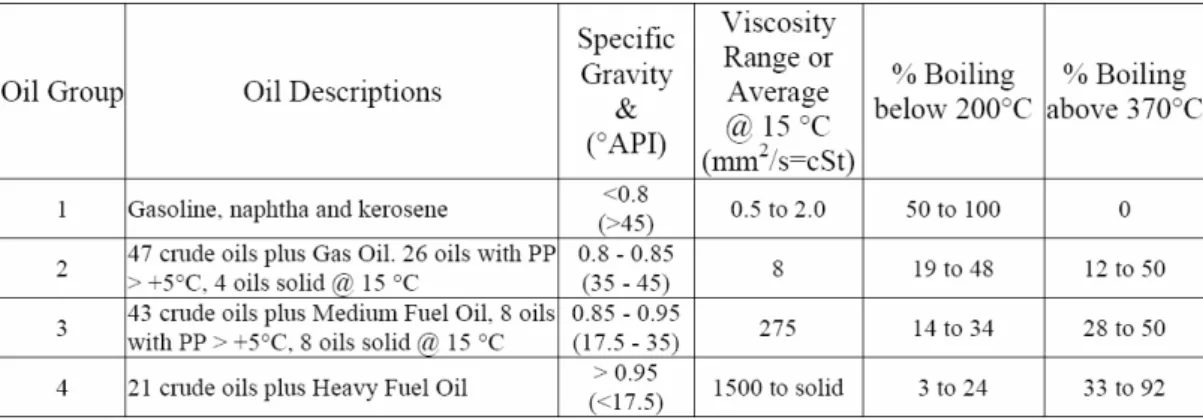
To adopt a worst case condition for the oil spill, the choice of the oil type is essential. Light oils generally evaporate faster and disperse more readily into the water column. A heavy oil type that is subject to emulsification, low evaporation and dispersion rates, will result in larger amounts of oil that remain floating. Floating oil is in general perceived to be most directly damaging to the environment, because of the potential effects on birds and coastline. For the simulations that are carried out in this study, the simulated oil has an initial viscosity of 1500 cSt, and is subject to emulsification, causing a stable mousse to develop. This type of oil represents a heavy crude from Group 4 (ITOPF classification-Table 4-1).
Table 4-1 – ITOPF Oil group classification
As mentioned earlier, a worst case approach was adopted for the initial simulations of the spilled oil and chemical. The worst case approach for the chemical is to consider it as a conservative tracer, meaning no decay or other processes that reduce the concentration, other than by dilution. This approach will, in general, overestimate concentrations of the chemical, but will provide a good impression of the maximum probable extent of a possible spil.
All particle tracking model simulations cover a 5-day period. This period was chosen because it allows sufficient time for a hypothetical spill near the OWEZ to reach the
Netherlands coast and because this period would allow sufficient response time to prepare for the effects of such as spill.
4.2
Simulation of a hypothetical oil spill
In order to understand the fate of a possible oil spill, it is necessary to model to spread of the oil across the water surface and in the water column in the hours and days following such a spill. For the purpose of studying the potential effects of such a hypothetical oil spill, we have assumed a large (but arbitrary) amount of oil to be spilled near the OWEZ as a result of a possible collision of a ship with one of the wind turbines of the wind farm. We have simulated a spill amount of 10,000 kg of heavy oil. This amount has been chosen for ease of simulation and for clarity of visualisation of the results. The results of these simulations are then combined with estimates of actual spill amounts and the risk of occurrence in the overall risk assessment in Chapter 5.
Results of the model can be linearly scaled to any size of oil spill within the validity range of 0.5 – 90,000 tons. In order to verify this assumption, various tests were performed. For the range of the validity of the process description, these tests have shown that the deviation of the different oil components is less than 0.1% of the total amount of spilled oil. The travel times from the spill location to the coastline are not significantly affected by the amount of the spill.
The simulated amounts of floating oil and oil reaching the Netherlands coast can therefore be scaled to give actual expected amounts based on more realistic spill estimates arising from the risk assessment. The simulation results plotted in this chapter provide indications of the maximum probable extent of spreading of a potential oil spill, the expected trajectory of the oil following the spill, locations along the Netherlands coast where the spilled oil may end up and travel times of the oil from the spill location to the coastline. For a real spill situation, the concentration values shown in the plots should be scaled to reflect the actual spilled amount. The plots may also easily be used to calculate the "relative" amounts of residual floating oil or beached oil that can be expected following a spill.
The fate and spread of an oil spill can be significantly affected by the actual weather conditions on the North Sea in the days immediately following the accident. We have investigated various scenarios to cover a wide range of possible weather conditions. Firstly, we have considered an "average" situation (constant south-west wind of 7 m/s), representative of the long-term conditions on the North Sea. Secondly, we have considered a severe storm condition (constant north-west wind of 17 m/s). Both of these first two scenarios consider a constant wind speed and direction for the entire duration of the simulation. It is recognised, however, that weather conditions on the North Sea are in fact quite variable.
We have therefore defined an additional scenario that takes into account a more variable wind pattern. This so-called "stochastic" simulation uses stochastic sampling to generate about 500 wind series from the long-term historical wind database of the area. For each of the generated wind series, the trajectory of the oil spill has been simulated for a 5-day period. By combining the results of all of these simulations, we arrive at a spatial map giving the probability (per km2) that oil may be present within the 5-day time frame. These
probability maps can be combined with the actual probability of a spill occurrence to arrive at estimates of actual risk to the local environment (see Chapter 5).
4.2.1 South-westerly wind of 7 m/s
After the spill, the oil is blown in a north-easterly direction towards the Dutch coast, and the first oil arrives at the coastline of northern Holland, 1 day after the spill. At the southern tip of Texel, the first oil arrives at about 2 days after the spill. Some of the oil enters the Waddenzee (Figure 4-2).
Figure 4-2 – Simulated maximum surface floating oil concentration (kg/m2), with a constant south-westerly wind
Figure 4-3 – Simulated amount of beached oil (kg/m2), with a constant south-westerly wind of 7m/s, 5 days after
the hypothetical oil spill
An analysis of the oil mass balance shows after 5 days that about 9% of the spilled oil has evaporated, 90% of the oil reaches the coastline and a small fraction (<0.5%) is oil that floats on the water and/or is dispersed in the water column. Most of the spilled oil (about 80%) reaches the coastline over a distance of about 20 km (Figure 4-3) and some on the southern tip of Texel. The remainder of the oil is distributed over a larger area and reaches the coast in relatively small quantities.
The amount of oil that is being dispersed into the water column is very small, hence no significant amounts of oil will attach to the sediments and seabed.
4.2.2 North-westerly wind of 17 m/s
The effects of the oil spill during north-westerly storm conditions (17 m/s), the oil is transported in a south-easterly direction (Figure 4-4). The main part of the surface oil patch travels in the direction of IJmuiden harbour and the first oil reaches it within 10 hours after the spill. About 80% of the oil beaches in the vicinity of the harbour (over a distance of less than 10 km), Figure 4-5. About 4% of the oil evaporates whilst about 10% sticks to the sea bottom over a relatively large area of about 20 by 30 km. Due to the strong wind conditions, more oil disperses into the water column compared to the 7 m/s wind condition. Some of the dispersed oil will reach the seabed and sticks to the sediment over a relatively large area.
Figure 4-4 – Simulated maximum surface floating oil (kg/m2), with a constant north-westerly wind of 17m/s, 5
Figure 4-5 – Simulated amount of beached oil (kg/m2), with a constant north-westerly wind of 17m/s, 5 days
after the hypothetical oil spill
4.2.3 Stochastic simulation of an oil spill
A third simulation was carried out with the aim to estimate the probability of the oil distribution, including beaching, assuming an oil spill has occurred. This is achieved by running the oil model in a stochastic mode, in which the most important driving force, the wind, is randomly taken from a long wind record, with hourly observations, from IJmuiden (Source KNMI, The Netherlands) and represents the general conditions in this area. The
data covers a 50-year period. The last 6 years of this dataset are summarised in a windrose (Figure 4-6), showing that the most dominant wind direction is from the south west. The most frequent wind speed from that direction is between 5 and 10 m/s.
0.0% 5.0% 10.0% 15.0% 20.0% 25.0% North Northeast East Southeast South Southwest West Northwest >15 m/ s 15.0 m/s 10.0 m/s 5.0 m/s 2.0 m/s 1.0 m/s Ijm uiden data
1-jan-1999 to 1-jan-2005
Source: KNMI, The Netherlands
Figure 4-6 – Windrose for IJmuiden (1999-2005)
At random, 500 complete wind time series were selected from the observed record and used in a stochastic simulation. The same oil type as used in the previous simulations was introduced. The results are presented as probability of oil being present in an area of 1 km2 during the 5-day simulation (Figure 4-7 and Figure 4-9, for floating and beached oil respectively). The associated travel times are in Figure 4-8 and Figure 4-10.
From the stochastic simulation, it appears that the coastline north of IJmuiden would be most at risk from oil pollution, in case of an oil release due to a collision with the wind turbines. Overall there is about 21% probability that oil will reach the coastline within 5 days, in case of such an oil spill. The results also show that in general the first oil may reach the coast in about 18 hours, which is an indication of the response time that is available before the beaches are polluted.
It should be mentioned that these figures are assuming an oil spill has happened. For an actual assessment of the risks, these numbers must be multiplied with the probability of an oil spillage (risk = probability * impact).
Figure 4-10 –Estimated arrival time of beached oil of a hypothetical oil spill
4.3
Effects of a hypothetical chemical spill
A hypothetical spill was simulated by assuming no decay, which constitutes a worst-case approach in terms of environmental effects. The meteorological conditions and hydrodynamics of the simulations of the two hypothetical chemical spills are the same as for the oil spills (Section 4.2), one case with a 7 m/s south-westerly wind and the second with a 17 m/s north-westerly wind.
The hypothetical spill involves an instantaneous release of 1000 (units) and is released at the water surface. It is assumed that the density of the chemical is the same as that of seawater. Since the substance is assumed to behave as a conservative tracer, the results can be scaled to an actual release and hence the units of the release are not relevant.
4.4
South-westerly wind of 7 m/s
The effect of the wind on the dispersion of the conservative tracer is significantly less than for the surface floating oil. The main driving force of the advection is the current, which in part is affected by the wind, but has a significant tidal component. The effect of the wind is particularly noted by the residual currents that are directed north and as a result, the plume from the discharge is also directed north (Figure 4-11).
The concentrations that are simulated reduce rapidly due to the advection and mixing. It is noted that the concentration field in Figure 4-11 is depth averaged. It is assumed here that there is no difference in density between the seawater and the pollutant, and that the pollutant mixes relatively quickly across the entire depth.
Figure 4-11 – Simulated maximum depth averaged tracer concentration with a south-westerly wind of 7m/s for a hypothetical chemical spill
4.4.1 North-westerly wind of 17 m/s
The strong north-westerly wind causes the residual current along the Dutch coast to reverse, compared with the south-westerly wind conditions. This is clearly visible in the maximum concentration plot (Figure 4-12). It can be seen that the size of the affected area is approximately the same as in Figure 4-11). Only for the lowest concentration contour the affected area is larger, but it should be noted that this represents a dilution factor of 108 to 109.
Figure 4-12 – Simulated maximum depth averaged tracer concentration, with a north-westerly wind of 17m/s for a hypothetical chemical spill
5 Long term expected risk of pollution due to
the OWEZ
5.1
Introduction
In the previous Chapter 3 presented results of the study, conducted by MARIN, into quantifying the effects of shipping with the presence of the wind farm. In this Section, the results of this activity, in combination with the modelling that was carried out (Section 4), will be used to estimate the long-term expected risk (e.g. in terms of expected annual amounts of stranded oil along the Dutch shoreline).
5.2
Risk of oil spillages
Oil pollution in the North Sea is observed frequently. In the Annual Report 2004 of the Dutch coastguard, 137 pollution incidents involving mineral oil were reported with a total volume of 115 m3.
In Chapter 3 a detailed description is given of the calculated probabilities of collisions and spills. For the assessment of the long term risks in terms of pollution, the most important information is the size of the spill and its probability of occurrence. It is assumed that spillages do not occur after ramming (i.e. frontal collisions), but may occur after drifting.
The results also indicate that the probability of a collision for each windturbine is approximately similar. Hence the overall risk of drifting for the entire windfarm is used, which means that the probability of drifting, taken from Table 3-2, for route-bounded ships is taken as 0.007812 (once every 128 years) and for non-route-bounded ships 0.00297 (once every 337 years).
The probabilities of bunker oil releases are about 10 times that of a cargo oil release, even though the mean spill per year is about the same. This is due to the fact that the amount of oil releases are significantly larger when it is a cargo oil release, rather than a bunker oil release.
The Tables indicate that the risk of an oil release due to a collision with the wind farm is very small. A release of oil (combining Table 3-6 and Table 3-7) is calculated to occur once every 2500 years. The additional risk of a spillage due to the wind farm compared with the existing risk is less than 0.1% (Table 3-8). The highest risk are with relatively small discharges (release of bunker oil of 150-750 m3 of oil), but these probabilities are very small (once every 5500 years).
In Chapter 4, it is estimated that the general probability that oil will reach the coastline within 5 days after a spill is approximately 21.5%. For the period from the spill to 5 days after the spill the risk that oil will reach the coast increases. The evolution of the risk of oil reaching the coastline with time is shown in Figure 5-1.
0 5 10 15 20 25 0 12 24 36 48 60 72 84 96 108 120 Time (hours) C P (%) 0 0.15 0.3 0.45 0.6 0.75 dC P/ dt (% /h our) Cum. probability (CP) dCP/dt
Figure 5-1 – Temporal development of the total (black line) and hourly (blue line) risk of coastal oil pollution, given a hypothetical oil spill
From Figure 5-1, it can be seen that the risk of oil reaching the coastline within 18 hours is insignificant and that it is most likely that oil will reach the coast between 36 and 51 hours. The increase of the hourly risk value around 96 hours after the spillage represents the arrival of the oil on the beaches of Texel. The probability of oil, given an oil release at the wind farm, reaching Texel is estimated at less than 1%.
Since it is estimated that there is a 21.5% probability that oil will reach the Dutch coast within 5 days (given an oil spill), reduces the frequency that oil will reach the Dutch coast due to a collision with the wind farm from once every 2500 years to about once every 12,000 years. For a scenario as described in Section 4.2.2, which would lead to oil in the vicinity of IJmuiden harbour, this risk is significantly smaller, when considering that the probability of wind from the North-west is about 10% (not taking wind speed into account). This reduces the risk of e.g. IJmuiden to be affected by an oil spill due to a collision with the wind farm to the order of once every 120,000 years. If the winds from whole of the north-western quadrant are used (probability of 36%) then this risk would be in the order of once every 35,000 years.
When the Dutch coastal area is sub-divided into zones, South of IJmuiden, North of IJmuiden, and the Waddenzee (including the coastlines of the islands), then the probabilities (given a spill has occurred) and return periods can be derived (Table 5-1).
Coastal Zone Probability (%) that oil will reach
the coast
Risk expressed in once every … years
Wadden 0.03 8·106
North of IJmuiden 19.8 12,600
South of IJmuiden 0.7 350,000
Total 21.5 11,600
Table 5-1 – Probabilities, for a given oil spill, and return periods of coastal oil pollution due to