Feature and Decision Level Fusion Using Multiple Kernel Learning and Fuzzy Integrals

(1)

Michigan Technological University Michigan Technological University

Digital Commons @ Michigan Tech

Dissertations, Master's Theses and Master's Reports

2017

Feature and Decision Level Fusion Using Multiple Kernel Learning

and Fuzzy Integrals

Tony Pinar

Michigan Technological University, [email protected]

Pinar, Tony, "Feature and Decision Level Fusion Using Multiple Kernel Learning and Fuzzy Integrals", Open Access Dissertation, Michigan Technological University, 2017.

(2)

FEATURE AND DECISION LEVEL FUSION USING MULTIPLE KERNEL LEARNING AND FUZZY INTEGRALS

By

Anthony J. Pinar

A DISSERTATION

Submitted in partial fulﬁllment of the requirements for the degree of DOCTOR OF PHILOSOPHY

In Electrical Engineering

MICHIGAN TECHNOLOGICAL UNIVERSITY 2017

(3)

(4)

This dissertation has been approved in partial fulﬁllment of the requirements for the Degree of DOCTOR OF PHILOSOPHY in Electrical Engineering.

Department of Electrical and Computer Engineering

Dissertation Advisor: Dr. Timothy C. Havens

Committee Member: Dr. Jeremy Bos

Committee Member: Dr. Timothy Schulz

Committee Member: Dr. Thomas Oommen

(5)

(6)

Dedication

To Noelle and Malcolm

(7)

(8)

List of Figures

1.1 High-level block diagram of feature-level fusion. . . 4

1.2 High-level block diagram of decision-level fusion. . . 5

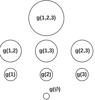
2.1 Lattice of FM elements for n= 3. Monotonicity (P5) is illustrated by the size of each circle, i.e., g({x₁})≤g({x₁, x₂}) as {x₁} ⊂ {x₁, x₂}. 22

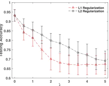
2.2 DeFIMKL performance using regularization on Sonar data. Error bars indicate ± one standard deviation. . . 46

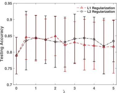
2.3 DeFIMKL performance using regularization on Dermatology data— classes {1,2,3} versus {4,5,6}. Error bars indicate ± one standard deviation. . . 47

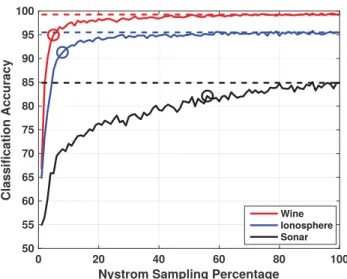
2.4 Results of using GAMKL₁on the Wine, Ionosphere, and Sonar datasets with the Nystr¨om approximation. Dashed line indicates full sample performance; circle indicates sample percentage at which performance drops 5%. . . 50

(17)

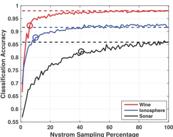
2.5 Results of using GAMKL₂on the Wine, Ionosphere, and Sonar datasets with the Nystr¨om approximation. Dashed line indicates full sample performance; circle indicates sample percentage at which performance drops 5%. . . 50

2.6 Results of using DeFIMKL₁ on the Wine, Ionosphere, and Sonar datasets with the Nystr¨om approximation. Dashed line indicates full sample performance; circle indicates sample percentage at which per-formance drops 5%. . . 51

2.7 Results of using DeFIMKL₂ on the Wine, Ionosphere, and Sonar datasets with the Nystr¨om approximation. Dashed line indicates full sample performance; circle indicates sample percentage at which per-formance drops 5%. . . 51

2.8 Average speed-up percentages of classiﬁers using the Nystr¨om approx-imation. . . 52

2.9 DeFIMKL performance using regularization on MNIST data. Error bars indicate± one standard deviation. . . 54

3.1 Lattice of FM elements for n= 3. Monotonicity (P5) is illustrated by the size of each node, i.e., g({x₁}) ≤ g({x₁, x₂}) as {x₁} ⊂ {x₁, x₂}. Note that shorthand notation is used where g(1,3) is equivalent to

(18)

3.2 The path taken by the Choquet integral due to a single input induc-ing the permutation π = {2,1,3}. Note that the FM was arbitrarily deﬁned in this example, and their distribution (ordering) follows that

of Figure 3.1. . . 69

3.3 Lattice of learned FM and paths for random training data from the Ionosphere data set usingm= 10. Note there are numerous untouched nodes and their learned values are driven by the constraints in (3.9). 69 4.1 Experiment 1 results. (a,b) Learned FM values in lexicographical order for λ = 0 to 50. Bin 1 is u(1) = g(x₁), bin N + 1 is u(N + 1) = g({x₁, x₂}), etc. Height of bar indicates FM value; color indicates λ value. (c,d) Plots showing performance of each regularization method in terms of SSE and Gini-Simpson index of the learned FM at each regularization parameter λ. . . 130

(a) Learned FM values using Gini-Simpson regularization . . . 130

(b) Learned FM values using ₁ regularization . . . 130

(c) Gini-Simpson regularization performance plots . . . 130

(19)

4.2 Experiment 2 results. (a,b) Learned FM values in lexicographical or-der. Bin 1 is u(1) = g(x₁), bin N + 1 is u(N + 1) = g({x₁, x₂}), etc. Height of the bar indicates FM value; color indicates λ value. (c,d) Plots showing performance of each regularization method in terms of SSE and Gini-Simpson index values of the learned FM at each

regu-larization parameter λ. . . 133

(a) Learned FM values using Gini-Simpson regularization . . . 133

(b) Learned FM values using ₁ regularization . . . 133

(c) Gini-Simpson regularization performance plots . . . 133

(d) ₁ regularization performance plots . . . 133

4.3 Experiment 3 results. Learned FM values in lexicographical order for Experiment 1. Bin 1 is u(1) = g(x₁), bin N + 1 is u(N + 1) = g({x₁, x₂}), etc. Height of the bar indicates FM value; color indicates iteration number. Plot of the Shapley values of the learned FM for Experiment 1 at each iteration. . . 134

(a) Learned FM values using iteratively reweighted₁ regularization for Experiment 1 . . . 134

(b) Shapley values for (a) . . . 134

(20)

5.2 An image contaminated with a large amount of noise and its low-rank and sparse decomposition. . . 148 5.3 The low-rank and sparse decomposition of an image with only one pixel

contaminated with a large amount of noise. . . 149 5.4 NAUC . . . 153 5.5 Examples of typical GPR data visualization . . . 154 5.6 Sparse component of GPR B-scan from Figure 5.5(b), computed using

RPCA . . . 155 5.7 Returned energy for a single sweep across a lane, over a target. Vertical

lines indicate the region in which the target is buried. . . 157 5.8 Example calculation of the peak SCR . . . 158 5.9 Unprocessed target B-scan used in Figures 5.10 and 5.12 . . . 165 5.10 A single B-scan processed with PCP-AD using multiple values for λ

along with the integrated energies. Note that image is labeled either

time orfrequency, corresponding to the domain in which the PCP-AD

algorithm was implemented. Dashed vertical lines denote the target region. . . 166 5.11 Eﬀect of the tuning parameter on the SCR when using PCP-AD. Note

that the frequency domain trace is clamped to zero for situations where computing the SCR is numerically limited, i.e., in cases where 0/0 is approached. . . 167

(21)

5.12 A single B-scan processed with OP-RPCA in the time domain using multiple values forλ along with the integrated energies. Dashed

verti-cal lines denote the target region. . . 168

5.13 Eﬀect of the tuning parameter on the SCR when using OP-RPCA. 169 5.14 Scattered plot of integrated A-scan energy for Lane A, GPR Channel 1. . . 171

5.15 Linear interpolation of scatter plot in Figure 5.14. . . 172

5.16 Results of applying clutter removal with m = 0.85 to Figure 5.14. . 172

5.17 Ascan . . . 175

5.18 Ascan . . . 177

5.19 CCMExample . . . 180

5.20 Sub-image at hit candidate location. . . 182

5.21 Gradient calculation with 3×3 cell arrangement. . . 183

5.22 Cell based 9-bin HOG feature. . . 184

5.23 freqPartition . . . 187

5.24 FFSTﬁlters . . . 187

5.25 NAUC . . . 190

5.26 prelanes . . . 192 5.27 Integrated energy ground map and an example queue point with 10,

(22)

5.28 DeFIMKL performance using regularization. Error bars indicate±one standard deviation. . . 208

(23)

(24)

List of Tables

2.1 Acronyms and Select Notation . . . 16 2.2 UCI Benchmark Data Sets . . . 29 2.3 RBF Kernel Parameter Ranges . . . 43 2.4 Classification Accuracy Results on Benchmark Data Sets* . . . 58 2.5 Additional Data Sets for Nyström Verification . . . 59 2.6 Nyström Sampling Percentage Required to Achieve Equivalent

Classi-ﬁcation Results as Full Sample . . . 59

3.1 Underlying and learned FMs (excludingg({∅}) andg(X) whose values are 0 and 1, respectively, due to the boundary conditions). The learned FM terms marked with an asterisk are not addressed by the training data. Regularization labels indicate the type of norm employed and the aggregation goal. For example, “₁-min” indicates a goal of that for minimum aggregation (g=0) and₁-regularization (u−g₁). 78 3.2 Classiﬁcation Accuracy of Various Regularization Functions* . . . . 92

4.1 Numeric Examples, for N = 3, Illustrating ₀ and Gini-Simpson Dif-ferences. . . 117

(25)

4.2 RBF Kernel Parameter Ranges and Data Set Properties . . . 137 4.3 Classiﬁer Performances—Means and Standard Deviations . . . 137

5.1 Average SCR over all targets* . . . 160 5.2 Average SCR over all wire targets* . . . 161 5.3 Average SCR over all landmine targets* . . . 161 5.4 Average SCR over all pressure plate targets* . . . 162 5.5 Average SCR over all main charge targets* . . . 163 5.6 Average RPCA decomposition time per sweep in seconds* . . . 164 5.7 Length of Features and Full Feature Set. . . 181 5.8 Results of CFAR Prescreener on each Channel and Lane. . . 191 5.9 NAUCs for the ROCs. . . 193 5.10 Results of SKSVM Classiﬁer on each Channel and Lane using Diﬀerent

Features—Prescreener Hits. . . 195 5.11 Results of SKSVM Classiﬁer on each Channel and Lane using Diﬀerent

Features—CCM Hits. . . 196 5.12 Results of SKSVM Classiﬁer on each Channel and Lane using Diﬀerent

Features—RP + CCM Hits. . . 197 5.13 Results of MKLSVM Classiﬁer on each Channel and Lane using

Dif-ferent Features—Prescreener Hits. . . 198 5.14 Results of MKLSVM Classiﬁer on each Channel and Lane using

(26)

5.15 Results of MKLSVM Classiﬁer on each Channel and Lane using Dif-ferent Features—RP + CCM Hits. . . 200 5.16 Summary of Best Results. . . 201 5.17 NAUCs and percentage improvement compared to the prescreener*. 207

(27)

(28)

Preface

Some chapters of this dissertation contain published material. The following list indicates which publications were used along with notes on author contributions.

Chapter 2

A. Pinar, T.C. Havens, D.T. Anderson, and L. Hu (2015). “Feature and decision level fusion using multiple kernel learning and fuzzy integrals,” Proc. FUZZ-IEEE, Aug 2015, pp. 1–7. (See [1].)

A.J. Pinar is the leading researcher in this work and is the corresponding author. The research was performed under the guidance of T.C. Havens, and the ideas proposed in the paper stemmed from conversations with D.T. Anderson and L. Hu.

A.J. Pinar, J. Rice, L. Hu, D.T. Anderson, and T.C. Havens (2016). “Eﬃcient multiple kernel classiﬁcation using feature and decision level fusion,” IEEE Trans.

Fuzzy Systems, Vol. PP. (See [2].)

A.J. Pinar is the leading researcher in this work and is the corresponding author. The research was performed under the guidance of T.C. Havens, and the ideas proposed

(29)

in the paper stemmed from conversations with D.T. Anderson and L. Hu. J. Rice contributed ideas to improve the implementation of the various algorithms discussed in the paper.

Chapter 3

A.J. Pinar, T.C. Havens, M.A. Islam, and D.T. Anderson (2017). “Visualization and learning of the Choquet integral with limited training data,” To appear, Proc.

FUZZ-IEEE.

A.J. Pinar is the leading researcher in this work and is the corresponding author. The research was performed under the guidance of T.C. Havens, and the ideas proposed in the paper stemmed from conversations with D.T. Anderson and M.A. Islam.

A.J. Pinar, T.C. Havens, M.A. Islam, and D.T. Anderson (2017). “Learning the Choquet Integral with a goal,” In preparation, IEEE Trans. Fuzzy Systems.

A.J. Pinar is the leading researcher in this work and is the corresponding author. The research was performed under the guidance of T.C. Havens, and the ideas proposed in the paper stemmed from conversations with D.T. Anderson and M.A. Islam.

(30)

Chapter 4

A.J. Pinar, D.T. Anderson, A. Zare, T.C. Havens, and T. Adeyeba (2017). “Measures of the Shapley Index for Learning Lower Complexity Fuzzy Integrals,” In review,

Springer Granular Computing.

The ideas presented in this paper are the result of discussions between all listed au-thors. A.J. Pinar is the corresponding author for this paper and generated the ex-perimental results. D.T. Anderson and T.C. Havens contributed the theoretical back-ground.

Chapter 5

A. Pinar, T.C. Havens, J. Rice, M. Masarik, J. Burns, and B. Thelen (2016). “A comparison of robust principal component analysis techniques for buried object de-tection in downward looking GPR and EMI sensor data,” Proc. SPIE, pp. 98230T. (See [3].)

A.J. Pinar is the leading researcher in this work and is the corresponding author. The research was performed under the guidance of T.C. Havens, and J. Rice assisted with the code written for the experiments. M. Masarik, J. Burns, and B. Thelen provided

(31)

data for use in the experiments.

A.J. Pinar, J. Rice, T.C. Havens, M. Masarik, J. Burns, and D.T. Anderson (2016). “Explosive hazard detection with feature and decision level fusion, multiple kernel learning, and fuzzy integrals,” Proc. IEEE CISDA, pp. 1–8. (See [4].)

A.J. Pinar is the leading researcher in this work and is the corresponding author. The research was performed under the guidance of T.C. Havens, and J. Rice assisted with the code written for the experiments. M. Masarik and J. Burns provided data for use in the experiments, and D.T. Anderson provided guidance with the theoretical components of the paper.

A. Pinar, M. Masarik, T.C. Havens, J. Burns, B. Thelen, and J. Becker (2015). “Ap-proach to explosive hazard detection using sensor fusion and multiple kernel learning with downward-looking GPR and EMI sensor data,” Proc. SPIE, pp. 94540B. (See [5].)

A.J. Pinar is the leading researcher in this work and is the corresponding author. The research was performed under the guidance of T.C. Havens, and M. Masarik, J. Burns, and B. Thelen provided data and algorithms for use in the experiments. Some ideas in this work originated in conversations with J. Becker.

(32)

Abstract

The work collected in this dissertation addresses the problem ofdata fusion. In other words, this is the problem of making decisions (also known as the problem of

classiﬁ-cation in the machine learning and statistics communities) when data from multiple

sources are available, or when decisions/confidence levels from a panel of decision-makers are accessible. This problem has become increasingly important in recent years, especially with the ever-increasing popularity of autonomous systems outfitted with suites of sensors and the dawn of the “age of big data.” While data fusion is a very broad topic, the work in this dissertation considers two very specific techniques:

feature-level fusion and decision-level fusion. In general, the fusion methods

pro-posed throughout this dissertation rely on kernel methods and fuzzy integrals. Both are very powerful tools, however, they also come with challenges, some of which are summarized below. I address these challenges in this dissertation.

Kernel methods for classiﬁcation is a well-studied area in which data are implicitly mapped from a lower-dimensional space to a higher-dimensional space to improve classiﬁcation accuracy. However, for most kernel methods, one must still choose a kernel to use for the problem. Since there is, in general, no way of knowing which kernel is the best, multiple kernel learning (MKL) is a technique used to learn the

(33)

aggregation of a set of valid kernels into a single (ideally) superior kernel. The aggre-gation can be done using weighted sums of the pre-computed kernels, but determining the summation weights is not a trivial task. Furthermore, MKL does not work well with large datasets because of limited storage space and prediction speed. These challenges are tackled by the introduction of many new algorithms in the following chapters. I also address MKL’s storage and speed drawbacks, allowing MKL-based techniques to be applied to big data eﬃciently.

Some algorithms in this work are based on theChoquet fuzzy integral, a powerful non-linear aggregation operator parameterized by thefuzzy measure(FM). These decision-level fusion algorithms learn a fuzzy measure by minimizing a sum of squared error

(SSE) criterion based on a set of training data. The ﬂexibility of the Choquet integral comes with a cost, however—given a set ofN decision makers, the size of the FM the algorithm must learn is 2N. This means that the training data must be diverse enough to include 2N _{independent observations, though this is rarely encountered in practice.}

I address this in the following chapters via many diﬀerent regularization functions, a popular technique in machine learning and statistics used to prevent overﬁtting and increase model generalization. Finally, it is worth noting that the aggregation behav-ior of the Choquet integral is not intuitive. I tackle this by proposing a quantitative visualization strategy allowing the FM and Choquet integral behavior to be shown simultaneously.

(34)

Chapter 1 Introduction

Information fusion is a broad multi-disciplinary topic with many applications. Gen-erally, it refers to the process of aggregating multiple sets of data (or other type of information) all explaining a common “thing”. For example, in the case of an au-tonomous robot, the “thing” might be its environment and the data will likely be collected from a suite of heterogeneous sensors outﬁtted on the vehicle. The robot can gain full autonomy if there are algorithms present that can eﬀectively fuse the various data it collects, and make decisions based on their aggregation. Another example more related to the autonomous agents of our species is the discrimination of edible food versus inedible food. When presented with a nutritional candidate, humans use their inborn sensor suites to extract informative features regarding its edibility. For example, its smell may contain information regarding the candidate’s

(35)

freshness—if the candidate smells rotten, it is likely inedible. Sight allows humans to categorize the candidate which also helps the decision process—if it looks like other foods known to be edible, it may also be edible. Ultimately, humans combine the information gathered by these senses (and others) to make the decision to eat or not to eat.

The above examples are examples of data-level or feature-level fusion, where the de-cision maker essentially combined the data before any dede-cisions were made. Another flavor of information fusion is decision-level fusion, where there exists a panel of de-cision makers, each making his or her own dede-cision based on the data at hand, and an overall decision is then determined through some process, e.g., voting. It is im-portant to note that in this context the decision can be a “confidence” or “rating.” A popular example of this type of fusion is the judging process in gymnastic or figure skating competitions—a panel of judges each rate the performance of a competitor by casting grades based on their own observations, and an overall score is assigned to the competitor by aggregating the judges’ ratings.

These high-level examples illuminate the two types of information fusion addressed in this dissertation: data-level fusion and feature-level fusion. The remainder of this chapter provides some context on how the low-level tools comprising the bulk of this dissertation fall under the roof of information fusion, and it will conclude with an outline of contributions. Furthermore, salient terminology is introduced and

(36)

explained throughout the chapter.

1.1 Problem Context

It is no coincidence that the high-level examples of the previous section ultimately ended with a decision; essentially all of the algorithms discussed in this disserta-tion are binary decision makers, i.e., binary classiﬁers.1 Hence, following the typical workﬂow for many machine learning or statistical prediction methods, the algorithms discussed later will betrained on a set of training data—data accurately labeled with known classes (labels) and is representative of the problem at hand, then tested on

testing data—data with unknown labels. The training process allows the classiﬁer to

learn the underlying model so that accurate predictions can be made on the testing data.

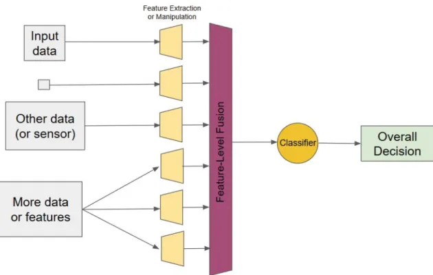
An example of a high-level feature-level fusion pipeline is shown in Figure 1.1. The input data, which can be from various sources or even a single source, is shown on the left and is fed into the first processing blocks that process the data in some way2. Next, the features are fused in some manner before a single classifier gives an overall decision. In the work that follows, I use an “off the shelf” classifier known as asupport

1_{While the classiﬁer I use in these algorithms is the} _{support vector machine} _{(SVM), generally any}

classiﬁer can be used in its place.

(37)

Figure 1.1: High-level block diagram of feature-level fusion.

vector machine (SVM), and the feature-level fusion algorithms I propose focus on the

feature fusion block just before classiﬁcation.

Figure 1.2 shows a similar block diagram for a decision-level fusion pipeline. Just as with feature-level fusion, the input data is on the left and is fed to some processing blocks. The difference here is that classification is performed before the fusion block; each processing block gets its very own classifier. The decisions generated by the different classifiers are then aggregated to form an overall decision by the fusion block. Again, the classifiers I use are SVMs and the decision-level fusion methods discussed later are included in the decision fusion block.

(38)

Figure 1.2: High-level block diagram of decision-level fusion.

The following sections briefly explain the tools used for fusion in the following chap-ters. Specifically, kernel SVMs and multiple kernel learning are discussed as the tools chosen for classification and feature-level fusion, respectively, and the Choquet fuzzy integral is introduced as the tool of choice for decision-level fusion.

1.1.1 SVMs and Kernels

A support vector machine is a type of binary classifier that finds a hyperplane in some space that discriminates between two classes of data; for linearly separable data, the SVM will work perfectly. This is not to say, however, that the SVM cannot be applied to more “complex” data—data that are not linearly separable can be accurately classified with a kernel SVM, i.e., a SVM that has been extended using

(39)

The kernel trick allows data to be nonlinearly mapped to a new higher-dimensional space termed the reproducing kernel Hilbert space (RKHS), where the data are (po-tentially) linearly separable. A linear classifier implemented in the RKHS can then perfectly discriminate the two classes. The SVM is one of the most popular classifiers to utilize the kernel trick since its formulation turns out to be very efficient—the nonlinear mapping can be performed implicitly through the use of kernel matrices, Hermitian matrices whose elements represent all pairwise inner products of the train-ing data. The elements of a kernel matrix are computed ustrain-ing a kernel function, which represents the inner product of two vectors in a RKHS defined by the kernel function chosen. There are many kernel functions to choose from, e.g., various radial

basis function kernels,polynomial kernels,sigmoidal kernels, etc., and they each have

at least one free parameter that must be chosen. This abundance of choice leads to the problem of determining which kernel (and parameter) to employ with the SVM. Recall that the goal of using a kernel is to project the data to a space where the data

are linearly separable, something not all kernels can achieve. This is the challenge

that multiple kernel learning (MKL) addresses.

MKL assumes that the kernel used as described in the previous paragraph is actually a linear combination of pre-selected base kernels. One must still choose the vari-ous base kernels with this MKL approach, but the process of learning the mixing coeﬃcients generally minimizes the inﬂuence of kernels that do not work well and

(40)

maximizes the contribution of kernels that do separate the data well. In a mathe-matical nutshell, given m base kernel matrices, Kk, MKL is the process of learning

the mixing coeﬃcients, σk, that form an “optimal” kernel as

K=

m

k=1

σkKk. (1.1)

The MKL algorithms in this dissertation all assume the formulation in (1.1), and many address the problem of learning a suitable set of mixing coeﬃcients. Appendix A provides a more quantitative discussion of SVMs including their kernel extension.

1.1.2 The Choquet Fuzzy Integral

Most of the decision-level fusion work in this dissertation uses the Choquet fuzzy

integral to combine the outputs of an ensemble of decision makers into a single overall

decision. This integral is extremely ﬂexible and is parametrized by thefuzzy measure

(FM), a function that maps the power set of all decision makers to the unit interval and can be thought of as the “worth” of a set. Therefore, we can say the Choquet fuzzy integral is “uber-parametrized,” since aggregating the decisions from a set of

m decision-makers using the integral requires 2m _{terms in its FM}3_{. Similar to MKL’s}

goal of learning the “optimal” mixing coeﬃcients based on training data, techniques

3_{Note that due to some properties of the FM, the number of required terms is actually 2}m₋_{2. This} will be explained in later chapters.

(41)

using the Choquet integral learn the FM that ﬁts the training data.

The number of required terms of the FM explodes as 2m_{, so learning the FM quickly}

becomes an underdetermined problem since sets of training data will rarely have the diversity to include 2m _{independent observations. This manifests as a learned FM}

that is only partially accurate—values of the FM driven by the training data are very accurately learned, but the remaining values are driven only by constraints; their values are essentially erroneous. Thus, when faced with testing data that utilizes the incorrectly learned FM values the classiﬁcation accuracy will generally suﬀer.

Much of the work in the following chapters addresses this problem through the use of

regularization, a technique commonly used in machine learning to prevent overﬁtting.

Doing so reduces the influence of the constraints on the learned FM and rather reas-signs the influence to the regularization function; the choice of regularization function defines how the values of the FM not driven by training data are learned.

1.2 Dissertation Outline and Contributions

The following chapters summarize my work on the data fusion problem along with some application-speciﬁc contributions to ground penetrating radar (GPR). The re-mainder of this section describes each chapter more concretely and explains the novel

(42)

contributions of each chapter.

Chapter 2 proposes multiple feature-level and decision-level fusion algorithms,

demonstrates their performance when used with support vector machine classiﬁers, and proposes a general method for extending multiple kernel learning-based algo-rithms to large datasets through the use of the Nystr¨om approximation. Experimental results demonstrate the algorithms’ utility as well as validate their extension to “big data”. A decision-level fusion algorithm proposed in this paper, namely

decision-level fuzzy integral multiple kernel learning (DeFIMKL), is a common thread also

appearing in the chapters that follow.

Chapters 3 and 4 further extend the fuzzy integrbased decision-level fusion

al-gorithm introduced in Chapter 2 in many ways. The novelty in Chapter 3 allows

the algorithm’s behavior to be more ﬁnely “tuned” towards various aggregation op-erators, and that of Chapter 4 aims to improve the algorithm’s generalization by

penalizing its complexity during the learning process.

Chapter 5 applies some of the fusion techniques presented in this dissertation to

the problem of explosive hazard detection using ground penetrating radar (GPR). The chapter is broken into three parts—Part I presents an exploration of various robust

(43)

step. Next, Part II summarizes an approach to the detection process using

state-of-the-art fusion methods and providing a picture of the entire detection pipeline including prescreening, feature extraction, and classiﬁcation. Finally, Part III

ap-plies the fusion techniques from Chapter 2 to the GPR data.

Finally, Chapter 6 concludes the dissertation and discusses future work.

1.3 List of Relevant Publications

The research summarized in this dissertation is based on the following publications:

1. A. Pinar, T.C. Havens, D.T. Anderson, and L. Hu (2015). “Feature and decision level fusion using multiple kernel learning and fuzzy integrals,” Proc. FUZZ-IEEE, Aug 2015, pp. 1–7. (See [1].)

2. A.J. Pinar, J. Rice, L. Hu, D.T. Anderson, and T.C. Havens (2016). “Ef-ﬁcient multiple kernel classiﬁcation using feature and decision level fusion,”

IEEE Trans. Fuzzy Systems, Vol. PP. (See [2].)

3. A.J. Pinar, T.C. Havens, M.A. Islam, and D.T. Anderson (2017). “Visualization and learning of the Choquet integral with limited training data,” To appear,

(44)

4. A.J. Pinar, T.C. Havens, M.A. Islam, and D.T. Anderson (2017). “Learning the Choquet Integral with a goal,”In preparation, IEEE Trans. Fuzzy Systems.

5. A.J. Pinar, D.T. Anderson, A. Zare, T.C. Havens, and T. Adeyeba (2017). “Measures of the Shapley Index for Learning Lower Complexity Fuzzy Inte-grals,” In review, Springer Granular Computing.

6. A. Pinar, T.C. Havens, J. Rice, M. Masarik, J. Burns, and B. Thelen (2016). “A comparison of robust principal component analysis techniques for buried object detection in downward looking GPR and EMI sensor data,”Proc. SPIE, pp. 98230T. (See [3].)

7. A.J. Pinar, J. Rice, T.C. Havens, M. Masarik, J. Burns, and D.T. Anderson (2016). “Explosive hazard detection with feature and decision level fusion, multiple kernel learning, and fuzzy integrals,” Proc. IEEE CISDA, pp. 1–8. (See [4].)

8. A. Pinar, M. Masarik, T.C. Havens, J. Burns, B. Thelen, and J. Becker (2015). “Approach to explosive hazard detection using sensor fusion and multiple kernel learning with downward-looking GPR and EMI sensor data,” Proc. SPIE, pp. 94540B. (See [5].)

(45)

1. M.A. Islam, D.T. Anderson, A.J. Pinar, and T.C. Havens (2016).

“Data-driven compression and eﬃcient learning of the Choquet integral,” In review, IEEE Trans. Fuzzy Systems.

2. T.C. Havens, J. Becker,A. Pinar, and T.J. Schulz (2014). “Multi-band

sensor-fused explosive hazard detection in forward-looking ground-penetrating radar,”

Proc. SPIE, vol. 9072. (See [6].)

3. T.C. Havens, D.T. Anderson, K. Stone, J. Becker, and A.J. Pinar (2016).

“Computational Intelligence in Forward Looking Explosive Hazard Detection,” Chapter in Recent Advances in Computational Intelligence in Defense and

Se-curity. Berlin: Springer. (See [7].)

Proof of copyright permission for the necessary publications used in this dissertation are provided in Appendix C.

(46)

Chapter 2 Eﬃcient Multiple Kernel

Classiﬁcation using Feature and

Decision Level Fusion

The material in this chapter was previously published in IEEE Transactions on Fuzzy Systems, Vol. PP, no. 99, 2016.

(47)

2.1 Introduction

Consider a set of numericalfeature-vector data that has the formX ={x₁, . . . ,xn} ⊂

Rd_{, where the coordinates of} _x

i provide feature values (e.g., bits per second, speed,

volts, etc.) describing some object (e.g., a wireless sensor network node, traﬃc cam-era, or radar). We are also given a set of training labels for each feature vector, such that we have the pair (y, X), wherey= (y₁, . . . , yn)T andyi is the label ofith object.

Each yi is associated with a respective feature vector xi. The classiﬁer learning task

is thus to learn some prediction function f, such that we can predict the label of the feature-vectors, i.e., y=f(x).

Most classifiers delineate the classes by finding some “best” decision boundary in the feature space. Perceptrons and linear support vector machines (SVMs) find hyper-planes1. These classifiers are easy to train, often can be effective, and are compu-tationally very efficient (the operational decision is just a single dot-product in the feature space). However, they are ineffective for classes that are not linearly separa-ble, i.e., by a hyperplane. Hence, we will use kernel classifiers to non-linearly project the features into a high-dimensional space, where hyperplanes may be more easily found that serve as good decision boundaries.

(48)

its name implies, MKL combines multiple kernels together to form a new kernel, and thus a new classiﬁcation space. Furthermore, since kernels known to exploit the data’s various features can be used as building blocks for MKL, it can do very well with heterogeneous data. There are many works that discuss MKL [8, 9, 10, 11, 12, 13, 14], and nearly all of them rely on operations that aggregate kernels in ways that preserve symmetry and positive semi-deﬁniteness, such as element-wise addition and multiplication. Most MKL algorithms learn a “best” kernel space in which to classify by learning respective weights on each component kernel. Details are contained in Section 2.4.

Two MKL formulations explored in this chapter focus on aggregation using the

Cho-quet fuzzy integral (FI) with respect to a fuzzy measure (FM) [15]. First, we

inves-tigate our previously proposed fuzzy integral: genetic algorithm (FIGA) approach to MKL [11, 12], proving that it reduces to a special kind of linear convex sum (LCS) kernel aggregation. This leads to the proposition of the p-norm genetic algorithm

MKL (GAMKLp) approach, which learns an MKL classiﬁer using a genetic algorithm

and generalizedp-norm weight domain. These algorithms perform a feature-level ag-gregation of the kernel matrices, producing a new feature representation. We also propose a decision-level MKL called DeFIMKL, which learns a FM with respect to the Choquet FI to fuse decisions from individual kernel classiﬁers. The FM is learned from training data with a regularized quadratic program (QP) approach [16]. We

(49)

Table 2.1

Acronyms and Select Notation SVM support vector machine

MKL multiple kernel learning FM fuzzy measure

FI fuzzy integral

FIGA fuzzy integral: genetic algorithm LCS linear convex sum

GAMKLp p-norm genetic algorithm MKL

DeFIMKL decision-level fuzzy integral MKL

DeGAMKLp p-norm decision-level genetic algorithm MKL

DeLSMKL decision-level least squares MKL QP quadratic program

MKLGL MKL group lasso

MKLGLp MKLGL with p-norm regularization

RBF radial basis function

X feature-vector data, X ={x₁, . . . ,xn} ⊂Rd y data labels, y= (y₁, . . . , yn)T

f(x) prediction function

g fuzzy measure

π(i) sorting index in Choquet integral

φ(x) non-linear mapping of x

κ(xi,xj) kernel function, κ(xi,xj) = φ(xi)Tφ(xj) K kernel matrix K = [Kij =κ(xi,xj)] f_k(x) decision function using kth kernel, K_k

fg₍_x₎ _{decision function using Choquet integral, wrt FM} _g

further explore two additional decision-level methods based on a least-squares for-mulation. We start with decision-level least-squares MKL (DeLSMKL) where we compute the weights for decision values from an ensemble of classiﬁers using a closed form expression. We then extend this method using a nonlinear cost function and use a genetic algorithm to compute the weights in decision-level genetic algorithm MKL

(DeGAMKL).

(50)

Since the size of these kernels is directly related to the number of feature-vectors in the dataset, large datasets lead to large kernels. Thus, approximations to the kernel matrices that reduce the required number of values to store could allow MKL methods to be used for these large datasets. We explore the use of the Nyström approximation for this task, and show the effects of the approximation on classifier accuracy.

The FI-based MKL approaches are first compared with a leading machine learning MKL method, called MKL group lasso (MKLGL)2 [9] on several benchmark data sets. We also investigate the behavior of regularization on the results of DeFIMKL. In Section 2.2 we briefly review data fusion, and Section 2.3 introduces FMs and FIs, specifically the fuzzy Choquet integral. Section 2.4 details the MKL methods. A review of the preliminary experimental results generated in [17] are presented in Section 2.6, Section 2.7 presents the details and results of our Nyström experiments, and Section 2.8 discusses our final experiment with a large data set. Table 2.1 contains acronyms and selected notation used in this chapter.

2.2 Data Fusion

Data fusion is a broad term for methods that use multiple sets of data, perhaps data

from diﬀerent sensors or the output of multiple processes applied to the same data

(51)

set, to improve some performance metric from a baseline established using only one

set [18]. It is a very broad area of study, and there exists a vast pool literature relating to it; for a review of data fusion methods see [19] and [20]. Because of the breadth of the topic, we restrict this brief overview to the types of fusion techniques most related to the methods we employ.

Data fusion can be classiﬁed in many ways [21, 22, 23]. The taxonomy in [22] is most appropriate to apply to our approach, describing ﬁve categories of data fusion. The categories that encompass our fusion methods are termedfeature in—feature out

(FEI-FEO) anddecision in—decision out (DEI-DEO) and are brieﬂy discussed in the following sections.

2.2.1 Feature In—Feature Out Fusion

FEI-FEO fusion is also known as feature fusion, on which many computer vision meth-ods rely [24, 25, 26, 27]. A popular and powerful method of feature fusion combines the features in a multidimensional feature space using kernel methods [28, 29, 30, 31]. This allows the use of multiple kernels with classification, giving the advantage that particular kernels can exploit certain features better than other kernels. The SVM is a popular classifier for MKL classification, however comparable results have been shown using a logistic regression-based classifier [32].

(52)

2.2.2 Decision In—Decision Out Fusion

DEI-DIO fusion is commonly referred to as decision fusion. This approach is very closely related to concept of ensemble learning, where the decisions from multiple classifiers are combined to determine the overall decision. Indeed, this is precisely what the DeFIMKL algorithm discussed in Section 2.4.2 does. Due to the use of multiple classifiers, decision fusion is generally slower than feature fusion, which only requires one classifier [33].

Decision fusion can be done in two general ways: hard or soft. Hard decision fusion is done using the class labels from the ensemble of classifiers. A straightforward method of hard decision fusion is the majority vote approach. Soft decision fusion is performed using other outputs from the classifier ensemble such as the posterior probabilities, evidences, hypotheses, etc. A simple example in this case is to linearly combine the posterior probabilities [34]. Alternatively, for ensembles of fuzzy classifiers, the soft decision fusion approach could be used by aggregating the fuzzy class memberships determined by the classifiers [35].

(53)

2.3 Fuzzy Measures and Fuzzy Integrals

FIs and FMs have been proposed for many applications and for many types of data, from simple numeric data to intervals and type-2 fuzzy sets [36, 37, 38, 39, 40, 41, 42, 43, 44, 45, 46]. While manual specification of the FM works for small sets of sources (there are already 16 possible combinations of sources in the power set of 4 sources), manually specifying the values of the FM for large collections of sources is virtually impossible. Thus, automatic methods have been proposed, such as the Sugeno λ -measure [39] and the S-decomposable measure [47], which build the measure from the densities (the worth of individual sources), and genetic algorithm [11, 12, 38, 48], Gibbs sampling [49] and other learning methods [16, 50, 51], which build the measure by using training data. Other works [52, 53, 54] have proposed learning FMs that reflect trends in the data and have been specifically applied to crowd-sourcing, where the worth of individuals is not known, but extracted from the data.

2.3.1 Fuzzy measure

A measurable space is the tuple (X,Ω), where X is a set and Ω is a Ω-algebra or set of subsets of X such that

(54)

P1. X ∈Ω;

P2. ForA⊆X, if A∈Ω, then Ac _∈_Ω;

P3. If∀Ai ∈Ω, then

_∞

i=1Ai ∈Ω.

A FM is a function, g : Ω→[0,1], with the following properties:

P4. (Boundary conditions) g(∅) = 0 and g(X) = 1;

P5. (Monotonicity) IfA, B ∈Ω and A⊆B, then g(A)≤g(B).

If Ω is an inﬁnite set, then there is also a third property guaranteeing continuity; in practice and in this chapter, Ω is ﬁnite and thus this property is unnecessary. The FM values of the singletons, g({x_i}) = gi _{are commonly called the} _densities_{. Figure}

2.1 illustrates the lattice of a FM for the case of n= 3.

The arguably most popular FM is the Sugeno λ-measure, which has the attractive property of being able to be deﬁned completely by the values of the densities. The

λ-measure has the following additional property. For A, B ∈Ω andA∩B =∅,

(55)

g(1) g(4) g(1,2) g(1,3) g(1,2,3) g(2,3) g(2) g(3)

Figure 2.1: Lattice of FM elements for n = 3. Monotonicity (P5) is

illustrated by the size of each circle, i.e., g({x₁}) ≤ g({x₁, x₂}) as {x₁} ⊂

{x₁, x₂}.

where it can be shown that λ can be found by solving [39]

λ+ 1 = n i=1 1 +λgi, λ >−1. (2.1b)

2.3.2 Fuzzy integral

There are many forms of the FI; see [39] for detailed discussion. In general, they are parametric aggregation operators based on the fuzzy measure, hence the selection of measure leads to a speciﬁc aggregation operators. In practice, FIs are frequently used for evidence fusion [48, 55, 56, 57, 58]. They combine sources of information

(56)

by accounting for both the support of the question (the evidence) and the expected worth of each subset of sources (as supplied by the FM g). Here, we focus on the fuzzy Choquet integral, proposed by Murofushi and Sugeno [59, 60]. Let h :X →R

be a real-valued function that represents the evidence or support of a particular hypothesis.3 The discrete (ﬁnite Ω) fuzzy Choquet integral is deﬁned as

C h◦g =Cg(h) = n i=1 h(xπ(i)) [g(Ai)−g(Ai−1)], (2.2)

where π is a permutation of X, such that h(xπ₍₁₎) ≥ h(xπ₍₂₎) ≥ . . . ≥ h(xπ₍n₎), Ai ={xπ(1), . . . , xπ(i)}, and g(A0) = 0 [15, 42]. Detailed treatments of the properties

of FIs can be found in [15, 42, 61]. We now move on to showing how MKL can be achieved using the FM and FI.

2.4 Multiple Kernel Learning

Consider some non-linear mapping function φ: xi →φ(xi)∈ RDK, where DK is the

dimensionality of the transformed feature vector φ(xi). For brevity, we will denote

φ(xi) as φi. With kernel algorithms, one does not need to explicitly transform xi,

one simply needs to represent the dot product φ(xi)·φ(xj) =κ(xi,xj). The kernel

function κ can take many forms, with the polynomial κ(xi,xj) = (xTi xj + 1)p and

3_{Generally, when dealing with information fusion problems it is convenient to have}_h_:_X _→_[0_,_1],

(57)

radial-basis-function (RBF) κ(xi,xj) = exp(σ||xi−xj||2) being two of the most well

known. Given a set of n feature-vectors X, one can thus construct an n×n kernel matrix K = [Kij = κ(xi,xj)]n×n. This kernel matrix K represents all pairwise dot

products of the feature vectors in the transformed high-dimensional spaceHK—called

the Reproducing Kernel Hilbert Space (RKHS).

There are many algorithms that use kernels to transform the input data to an appro-priate and useful space; in this chapter, we focus on kernel-based classiﬁcation, such as the SVM [62, 63]. Multiple kernel algorithms, such as MKLGL [9] and FIGA [11], take single kernel algorithms a step further by representing the feature-vector with multiple kernels and then combining them to produce a single decision output. The kernel combination can be computed in many ways, as long as the combination results in a Mercer kernel [64]. For the feature-level fusion algorithms in this chapter, we will assume that the kernel K is composed by a weighted combination of pre-computed kernel matrices, i.e.,

K=

m

k₌₁

σkKk, (2.3)

where there aremkernels andσk is the weight applied to thekth kernel. The domain

ofσis very important and many MKL implementations only work for a single domain. For example, Δ₂ = {σ ∈ Rm _: _σ

2 = 1, σk ≥ 0} is the ₂-norm MKL [8, 10, 13].

MKLGL [9] uses a generalized MKL instantiation that allows for an p-norm domain

(58)

an SVM on the resultant kernel K. FIGA [11] generalizes (2.3) by representing the computation ofK by the Choquet FI,

K=

m

k=1

[g(Ak)−g(Ak−1)]Kπ(k), (2.4)

where Ak = {Kπ₍₁₎, . . . , Kπ₍k₎} is a set of kernel matrices sorted by a base-learner

quality measure and the FM g is learned by a genetic algorithm (GA); in essence, the entries of K are each the result of a Choquet FI. In Section 2.4.1 we show that the FIGA algorithm is actually learning an LCS MKL and is equivalent to (2.3) with

σ ∈Δ₁; we will use this new discovery to propose the GAMKLp algorithm.

2.4.1 The GAMKL

_p

algorithm

The FIGA algorithm produces an MKL classifier by learning one on the composite kernel K with the Choquet FI as shown in (2.4). The final classification function is learned on the kernel K, and, in past works [11, 12, 17], we have used the SVM for this final learner. The basic steps of FIGA are as follows:

1. Compute kernel matrices Kk = [κk(xi,xj)]n×n, k = 1, . . . , m;

2. Train a base-learner (e.g., SVM) on each kernelKk and record the classiﬁcation

(59)

3. Collect sorting indices π, such that η_π₍₁₎ ≥η_π₍₂₎ ≥. . .≥η_π₍_k₎;

4. Use a GA to learn the FM g, such that the classiﬁcation accuracy of a learner (e.g., SVM) on K at (2.4) is maximized.

The ﬁtness of each chromosome in step 4) of FIGA is the classiﬁcation accuracy of the learner on K, while the genes are (m−1) distinct values of the FM.4 Because FIGA only learns the sorting π once, in step 2), the GA only needs to learn (m−1) FM values, g({Kπ(1)}), g({Kπ(1), Kπ(2)}), . . ., g({Kπ(1), . . . , Kπ(m−1)}); by property

P4,g(A₀) = 0 and g(Am) = 1. This leads to Proposition 1

Proposition 1. Since the sorting order π is only found once in step 2) of FIGA, the

Choquet integral at (2.4) can be rewritten as

K= m k=1 σπ(k)Kπ(k), (2.5) where σπ₍k₎ =g(Ak)−g(Ak₋₁).

Proof. Because the sorting is not updated, the setsAk also remain unchanged; hence,

the summation weight on Kπ₍k₎ is the subtraction of the FM values of the same sets

(no matter their values). Hence, we can attach a single weightσπ(k)to eachKπ(k). 4_{In [12], an additional gene was added to indicate diﬀerent types of FMs and a slightly better}

(60)

Remark 1. Proposition 1 shows that the FIGA kernel composition at (2.4) is

inde-pendent of the initial sorting byπbecause the summation at (2.5) can be performed in any arbitrary order and give the same result. Hence, step 3) of FIGA is unnecessary.

Proposition 2. In FIGA, the domain of σπ(k) is Δ1.

Proof. The ₁ norm of σ is

m k=1 σπ(k) = m k=1 g(Ak)−g(Ak−1) =g(Am)−g(A0) = 1. (2.6)

Furthermore, due to the monotonicity property (P5) of g,σπ₍k₎ =g(Ak)−g(Ak₋₁)≥

0.

Remark 2. Proposition 2 shows the domain of σ upon which FIGA learns. Taking

Propositions 1 and 2 together shows that FIGA is equivalent to using a GA to learn the weights σ∈Δ₁ in the kernel combination at (2.3).

In light of this discovery, we propose a GAMKLpalgorithm that uses a GA to learn the

weightsσ∈Δp of (2.3). Whenp= 1, we have shown that this is equivalent to FIGA.

However, because of our discoveries in Propositions 1 and 2, we can simplify and generalize FIGA to allow for learning σ in the generalized domain Δp. The genes of

(61)

To ensure the GAMKL_p genes lie in the _p-norm domain Δ_p, all candidate genes ˜σ

are p-norm normalized to formσ as

σ = σ˜ p _m i=1 |σ˜i|p . (2.7)

The ﬁtness of each chromosome in GAMKLp is the 5-fold cross-validation

classiﬁca-tion accuracy of the learning algorithm—in this chapter, an SVM—trained on each chromosome’s aggregated K.

Remark 3. While Propositions 1 and 2 show that FIGA is equivalent to GAMKL₁,

the GAMKLpalgorithm has the additional beneﬁt that the genes of each chromosome

are not constrained to be monotonically increasing (as in FIGA). Hence, GAMKLp

is algorithmically more simple.

In Section 2.6, we will further investigate the performance of GAMKLp for real-world

(62)

Table 2.2

UCI Benchmark Data Sets

Data Set

Sonar Dermatology Wine

No. of Objects 208 366 178

No. of Features 60 33 13

Binary Classes {1} vs. {2} {1–3}vs. {4–6} {1} vs. {2,3}

Ionosphere Ecoli Glass

No. of Objects 351 336 214

No. of Features 34 7 9

Binary Classes {0} vs. {1} {1–4}vs. {5–8} {1–3} vs. {4–6}

2.4.2 The DeFIMKL algorithm

Let fk(xi) be the decision-value on feature-vector xi produced by the kth classiﬁer

in an ensemble. The overall decision of the ensemble is computed by the Choquet integral, where the evidenceh is the set of decisions by the classiﬁer ensemble and g

encodes the relative worth of each classiﬁer in the ensemble. So, mathematically, the ensemble decision fg₍_x

i) on feature-vector xi with respect to the FM g is produced

by fg(x_i) = m k=1 f_π₍_k₎(x_i) [g(A_k)−g(A_k₋₁)], (2.8) where Ak = {fπ₍₁₎(xi), . . . , fπ₍k₎(xi)}, such that fπ₍₁₎(xi) ≥ fπ₍₂₎(xi) ≥ . . . ≥ fπ(m)(xi). This is a generalized classiﬁer fusion method that has been explored in

many previous works [45, 57, 58, 65].

(63)

sum-of-squared error (SSE) optimization, which we now brieﬂy describe. Let the SSE be deﬁned as E2 = n i₌₁ (fg(xi)−yi)2, (2.9)

where yi is the class label for xi. It can be shown that (2.8), as a Choquet integral,

can be reformulated as fg(xi) = m k=1 f_π₍_k₎(xi)−fπ(k+1)(xi) g(Ak), (2.10)

where fπ(m+1) = 0 [15]. The SSE can thus be expanded as

E2 = n i=1 H_xT iu−yi ₂ , (2.11a)

whereuis the lexicographically ordered FMg, i.e.,u = (g({x₁}), g({x₂}), . . . , g({x₁∪ x₂}), g({x₁∪x₃}), . . . , g({x₁∪x₂∪. . .∪xm}), and Hxi = ⎛ ⎜ ⎜ ⎜ ⎜ ⎜ ⎜ ⎜ ⎜ ⎜ ⎜ ⎜ ⎜ ⎜ ⎜ ⎜ ⎜ ⎜ ⎜ ⎝ .. . fπ(1)(xi)−fπ(2)(xi) .. . 0 .. . fπ₍m₎(xi)−0 ⎞ ⎟ ⎟ ⎟ ⎟ ⎟ ⎟ ⎟ ⎟ ⎟ ⎟ ⎟ ⎟ ⎟ ⎟ ⎟ ⎟ ⎟ ⎟ ⎠ , (2.11b)

(64)

where H_x_i is of size (2m ₋₁₎_×_{1 and contains all the diﬀerence terms} _f

π(k)(xi)− fπ(k+1)(xi) at the corresponding locations of Ak in u. We can now fold out the

squared term in (2.11a), producing

E2 = n i₌₁ uTH_x_iH_xT iu−2yiH T xiu+y 2 i =uTDu+fTu+ n i₌₁ y2_i, (2.12) D= n i=1 HxiH T xi, f =− n i=1 2yiHxi.

Note that (2.12) is a quadratic function; hence, we can add in the constraints on

u, such that it represents a FM, producing a constrained QP. We can write the

monotonicity constraint on u, according to properties P4 and P5, as Cu≤0, where

C = ⎛ ⎜ ⎜ ⎜ ⎜ ⎜ ⎜ ⎜ ⎜ ⎜ ⎜ ⎜ ⎜ ⎜ ⎜ ⎜ ⎜ ⎜ ⎜ ⎝ ΨT 1 ΨT 2 .. . ΨT n+1 .. . ΨT m(2m−1₋₁₎ ⎞ ⎟ ⎟ ⎟ ⎟ ⎟ ⎟ ⎟ ⎟ ⎟ ⎟ ⎟ ⎟ ⎟ ⎟ ⎟ ⎟ ⎟ ⎟ ⎠ (2.13) and ΨT

1 is a vector representation of the monotonicity constraint, g({x1})−g({x1∪

x₂}) ≤ 0. Hence, C is simply a matrix of {0,1,−1} values of size (m(2m−1 ₋₁₎₎_×

(65)

the FM u is

min u 0.5u

T_D_ˆ_u₊_fT_u_, _C_u_≤₀_, ₍₀_,₁₎T _≤_u_≤₁_, _(2.14)

where ˆD= 2D. We will also test the performance of ₂ and ₁ regularization on the optimization at (2.14), i.e.,

min u 0.5u

T_D_ˆ_u₊_fT_u₊_λ_u

p, (2.15)

wherep= 1 for₁ regularization and p= 2 for₂. Again, see [16] for more discussion on this topic. The QPs at (2.14) and (2.15) provide a method to learn the FMu(i.e.,

g) from training data. We now propose a method for using this learning method for ensemble learning with kernel SVMs.

We propose that each learner fk(xi) is a kernel classiﬁer, each trained on a separate

kernel Kk; here, we will use the SVM. The SVM classiﬁer decision value is

ηk(x) = n

i₌₁

αikyiκk(xi,x)−bk, (2.16)

which is the distance of x from the hyperplane deﬁned by the learned SVM model

parameters, αik and bk [62, 63]. Typically, the class label is then computed as

sgn{ηk(x)}. One could use fk(x) = sgn{ηk(x)} as the training input to the FM

learning at (2.12), but this eliminates information about which kernel produces the largest class separation—essentially, the diﬀerence between ηk(x) for classes labeled

Feature and Decision Level Fusion Using Multiple Kernel Learning and Fuzzy Integrals

Digital Commons @ Michigan Tech

Digital Commons @ Michigan Tech

Feature and Decision Level Fusion Using Multiple Kernel Learning

Feature and Decision Level Fusion Using Multiple Kernel Learning

and Fuzzy Integrals

and Fuzzy Integrals

Dedication

To Noelle and Malcolm

Contents

I

A Comparison of Robust Principal Component

Analy-sis Techniques for Buried Object Detection in Downward

Looking GPR Sensor Data

144

II

Approach to Explosive Hazard Detection Using

Sen-sor Fusion and Multiple Kernel Learning with

Downward-Looking GPR and EMI Sensor Data

170

III

Explosive Hazard Detection with Feature and

Deci-sion Level FuDeci-sion, Multiple Kernel Learning, and Fuzzy

Integrals

203

List of Figures

List of Tables

Preface

Chapter 2

Chapter 3

Chapter 4

Chapter 5

Abstract

Chapter 1

Introduction

1.1

Problem Context

1.1.1

SVMs and Kernels

1.1.2

The Choquet Fuzzy Integral

1.2

Dissertation Outline and Contributions

1.3

List of Relevant Publications

Chapter 2

Eﬃcient Multiple Kernel

Classiﬁcation using Feature and

Decision Level Fusion

2.1

Introduction

2.2

Data Fusion

2.2.1

Feature In—Feature Out Fusion

2.2.2

Decision In—Decision Out Fusion

2.3

Fuzzy Measures and Fuzzy Integrals

2.3.1

Fuzzy measure

2.3.2

Fuzzy integral

2.4

Multiple Kernel Learning

2.4.1

The GAMKL

algorithm

2.4.2

The DeFIMKL algorithm