https://doi.org/10.1007/s11634-019-00364-9
R E G U L A R A R T I C L E
Ensemble of optimal trees, random forest and random
projection ensemble classification
Zardad Khan1,2·Asma Gul2,3·Aris Perperoglou2·
Miftahuddin Miftahuddin2,4·Osama Mahmoud2,5,6·Werner Adler7· Berthold Lausen2
Received: 13 February 2018 / Revised: 27 May 2019 / Accepted: 4 June 2019 © The Author(s) 2019
Abstract
The predictive performance of a random forest ensemble is highly associated with the strength of individual trees and their diversity. Ensemble of a small number of accurate and diverse trees, if prediction accuracy is not compromised, will also reduce computational burden. We investigate the idea of integrating trees that are accurate and diverse. For this purpose, we utilize out-of-bag observations as a validation sample from the training bootstrap samples, to choose the best trees based on their individual performance and then assess these trees for diversity using the Brier score on an independent validation sample. Starting from the first best tree, a tree is selected for the final ensemble if its addition to the forest reduces error of the trees that have already been added. Our approach does not use an implicit dimension reduction for each tree as random project ensemble classification. A total of 35 bench mark problems on classification and regression are used to assess the performance of the proposed method and compare it with random forest, random projection ensemble, node harvest, support
vector machine,kNN and classification and regression tree. We compute unexplained
variances or classification error rates for all the methods on the corresponding data sets. Our experiments reveal that the size of the ensemble is reduced significantly and better results are obtained in most of the cases. Results of a simulation study are also given where four tree style scenarios are considered to generate data sets with several structures.
Keywords Ensemble classification·Ensemble regression·Random forest·Random
projection ensemble classification·Accuracy and diversity
B
Zardad KhanB
Berthold LausenMathematics Subject Classification 62-00·62-07
1 Introduction
Various authors have suggested that combining weak models leads to efficient
ensem-bles (Schapire1990; Domingos1996; Quinlan1996; Maclin and Opitz2011; Hothorn
and Lausen2003; Janitza et al.2015; Gul et al.2016b; Lausser et al.2016;
Bolón-Canedo et al.2012; Bhardwaj et al.2016; Liberati et al.2017). Combining the outputs
of multiple classifiers also reduces generalization error (Domingos 1996; Quinlan
1996; Bauer and Kohavi1999; Maclin and Opitz2011; Tzirakis and Tjortjis2017).
Ensemble methods are effective in that different types of models have different induc-tive biases where such diversity reduces variance-error while not increasing the bias
error (Mitchell1997; Tumer and Ghosh1996; Ali and Pazzani1996).
Extending this notion, Breiman (2001) suggested growing a large number,T for
instance, of classification and regression trees. Trees are grown on bootstrap samples
form a given training dataL=(X,Y)= {(x1,y1), (x2,y2), . . . , (xn,yn)}. Thexiare
observations ond features andyvalues are from the set of real numbers and a set of
known classes(1,2,3, . . . ,K)in cases of regression and classification, respectively.
Breiman called this method bagging and using random selections of features at each
node random forest (Breiman2001).
As the number of trees in random forest is often very large, there has been a signif-icant work done on the problem of minimizing this number to reduce computational
cost without decreasing prediction accuracy (Bernard et al.2009; Meinshausen2010;
Oshiro et al.2012; Latinne et al.2001a).
Overall prediction error of a random forest is highly associated with the strength of individual trees and their diversity in the forest. This idea is backed by Breiman
(2001) upper bound for the overall prediction error of random forest given by
Err ≤ ¯ρerrj, (1)
where j = 1,2,3, . . . ,T, T denotes the number of all trees,Err is the overall
prediction error of the forest, ρ¯ represents weighted correlation between residuals
from two independent trees i.e. mean (expected) value of their correlation over entire
ensemble, anderrj is the average prediction error of some jth tree in the forest.
Based on the above discussion, our paper proposes to select the best trees, in terms of individual strength i.e. accuracy and diversity, from a large ensemble grown by random forest. Using 35 benchmark data sets, the results from the new method are compared with those of random forest, random projection ensemble (classification case only),
node harvest, support vector machine,kNN and and classification and regression tree
(CART). For further verification, a simulation study is also given where data sets with many tree structures are generated. The rest of the paper is organized as follows. The proposed method, the underlying algorithm and some other related approaches are
given in Sect.2, experiments and results based on benchmark and simulated data sets
2 OTE: optimal trees ensemble
Random forest refines bagging by introducing additional randomness in the base models, trees, by drawing subsets of the predictor set for partitioning the nodes of
a tree (Breiman2001). This article investigates the possibility of further refinement by
proposing a method of tree selection on the basis of their individual accuracy and
diver-sity using unexplained variance and Brier score (Brier1950) in cases of regression and
classification respectively. To this end, we partition the given training dataL=(X,Y)
randomly into two non overlapping partitions,LB =(XB,YB)andLV=(XV,YV).
GrowT classification or regression trees onT bootstrap samples from the first
par-titionLB = (XB,YB). While doing so, select a random sample of p <d features
from the entire set ofdpredictors at each node of the trees. This inculcates additional
randomness in the trees. Due to bootstrapping, there will be some observations left out of the samples which are called out-of-bag (OOB) observations. These observations take no part in the training of the tree and can be utilized in two ways:
1. In case of regression, out-of-bag observations are used to estimate unexplained variances of each tree grown on a bootstrap sample by the method of random
forest (Breiman2001). Trees are then ranked in ascending order with respect to
their unexplained variances and the top rankedM trees are chosen.
2. In case of classification, out-of-bag observations are used to estimate error rates
of the trees grown by the method of random forest (Breiman2001). Trees are then
ranked in ascending order whith respect to their error rates and the top rankedM
trees are chosen.
A diversity check is carried out as follows
1. Starting from the two top ranked trees, successive ranked trees are added one by
one to see how they perform on the independent validation data,LV=(XV,YV).
This is done until the lastMth tree is tested.
2. Select tree Lˆk,k = 1,2,3, . . . ,M if its inclusion to the ensemble without the
kth tree satisfys the following two criteria given for regression and classification
respectively.
(a) In the regression case, let U.EX Pk− be the unexplained variance of the
ensemble not having thekth tree andU.EX Pk+be the unexplained variance
of the ensemble withkth tree included, then treeLˆk is chosen if
U.EX Pk+<U.EX Pk−.
(b) In the classification case, letBSˆ k−be the Brier score of the ensemble not
having thekth tree andBSˆ k+be the Brier score of the ensemble withkth tree
included, then treeLˆkis chosen if
ˆ
where ˆ BS = # of test cases i=1 yi− ˆP(yi|X) 2
total # of test instances ,
yiis the state ofyifor observationiin the(0,1)form andPˆ(y|X)is the binary
response probability of the ensemble estimate given the features.
These trees, named as optimal trees, are then combined and are allowed to vote, in case of classification, or average, in case of regression, for new/test data. The resulting
ensemble is named as optimal trees ensemble,OTE.
2.1 The Algorithm
Steps of the proposed algorithm both for regression and classification are
1. Take T bootstrap samples from the given portion of the training data LB =
(XB,YB).
2. Grow regression/classification trees on all the bootstrap samples using random forest method.
3. Rank the trees in ascending order with respect to their prediction error on
out-of-bag data. Choose the firstMtrees with the smallest individual prediction error.
4. Add theM selected trees one by one and select a tree if it improves performance
on validation data,LV =(XV,YV), using unexplained variance and Brier score
in cases of regression and classification as the respective performance measures. 5. Combine and allow the trees to vote, in case of classification, or average, in case
of regression, for new/test data.
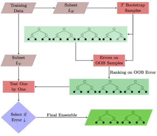
An illustrative flow chart of the proposed algorithm can be seen in Fig.1.
An algorithm, based on a similar idea has previously been proposed at the European Conference on Data Analysis 2014, where instead of classification trees, probability
estimation trees are used (Khan et al.2016). The ensemble of probability estimation
trees is used for estimating class membership probabilities in binary class problems. This paper, OTE, focuses on regression and classification and evaluates the perfor-mance by the standard measures of unexplained variances and classification error
rates. On the other hand, optimal trees ensemble given in Khan et al. (2016) is
focus-ing on probability estimation and provides comparison of the benchmark results by
Brier score. Moreover, we included a comparison of OTE and (Khan et al.2016),
OTE.Prob, (when evaluated by classification error rates) in the analysis of benchmark
problems in the last two columns of Table5of this paper.
Ensembles selection forkNN classifiers have also been proposed recently where in
addition to individual accuracy, thekNN models are grown on random subsets of the
Fig. 1 Flow chart ofOTEfor regression and classification
2.2 Related approaches
There has been a significant work done on the issue of reducing the number of trees in random forests by various authors. One possibility of limiting the number of trees in a random forest might be determining a priori the least number of trees to combine that gives prediction performance very similar to that of a complete random forest as
proposed by Latinne et al. (2001b). The main idea of this method is to avoid overfitting
trees in the ensemble. This method uses the McNemar test of significance to decide between the predictions given by two different forests having different number of trees.
Bernard et al. (2009) proposed a method of shrinking the size of forest by using two
well known selection methods: sequential forward selection method and sequential
backward selection method for finding sub-optimal forests. Li et al. (2010) proposed
the idea of tree weighting for random forest to learn data sets with high dimensions.
They used out-of-bag samples for weighting the trees in the forest. Adler et al. (2016)
have recently considered ensemble pruning to fix the class imbalanced problem by
using AUC and Brier score for Glaucoma detectection. Oshiro et al. (2012) examined
the performance of random forests with different numbers of trees on 29 different data sets and concluded that there is no significant gain in the prediction accuracy of a random forest by adding more than a certain number of trees. Zhang and Wang
(2009) considered the similarity of outcomes between the trees and removing the trees that were similar, thus reducing the size of the forest. They called this method the “By similarity method”. However, this method was not able to compete with their proposed “By prediction” method. Motivated by the idea of downsizing ensembles, this work has proposed optimal tree selection for classification and regression that could reduce computational costs and achieve promissing prediction accuracy.
3 Experiments and results
3.1 Simulation
This section presents four simulation scenarios each consisting of various tree
struc-tures (Khan et al.2016). The aim is to make the recognition problem slightly difficult
for classifiers likekNN and CART, and to provide a challenging task for the most
complex method like SVMs and random forest. In each of the scenarios, four different
complexity levels are considered by changing the weightsηi j kof the tree nodes.
Con-sequently, four different values of the Bayes error are obtained where the lowest Bayes error indicates a data set with strong patterns and the highest Bayes error means a data
set with weak patterns. Table1gives various values ofηi j kused in Scenarios 1, 2, 3,
and 4. Node weights for obtaining the complexity levels are listed in four columns of
the table fork =1,2,3,4, for each model. A generic equation for producing class
probabilities of the bernoulli responseY=Bernoulli(p)given then×3Tdimensional
vectorXofn ii dobservations from Uniform(0,1)is
p(y|X)= ex p c2× Zm T −c1 1+ex p c2× Zm T −c1 , whereZm = T t=1 ˆ pt. (2)
c1andc2are some arbitrary constants,m=1,2,3,4 is the scenario number andZm’s
aren×1 probability vectors.T is the total number of trees used in a scenario andpˆt’s
are class probabilities for a particular response inY. These probabilities are generated
by the following tree structures
ˆ
p1=η11k×1(x1≤0.5&x3≤0.5)+η12k×1(x1≤0.5&x3>0.5)+η13k×1(x1>0.5&x2≤0.5) +η14k×1(x1>0.5&x2>0.5),
ˆ
p2=η21k×1(x4≤0.5&x6≤0.5)+η22k×1(x4≤0.5&x6>0.5)+η23k×1(x4>0.5&x5≤0.5) +η24k×1(x4>0.5&x5>0.5),
ˆ
p3=η31k×1(x7≤0.5&x8≤0.5)+η32k×1(x7≤0.5&x8>0.5)+η33k×1(x7>0.5&x9≤0.5) +η34k×1(x7>0.5&x9>0.5),
ˆ
p4=η41k×1(x10≤0.5&x11≤0.5)+η42k×1(x10≤0.5&x11>0.5)+η43k×1(x10>0.5&x12≤0.5) +η44k×1(x10>0.5&x12>0.5),
ˆ
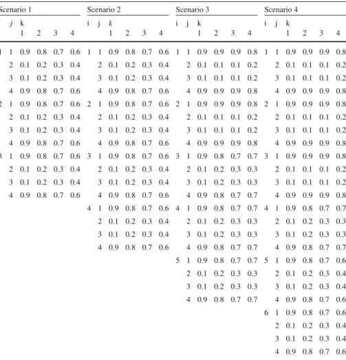
Table 1 Node weights,ηi j k, used in simulation scenarios whereiis the tree number,jis the node number in each tree andkis denoting a variant of the weights for the four complexity levels for all the scenarios (Khan et al.2016)
Scenario 1 Scenario 2 Scenario 3 Scenario 4
i j k i j k i j k i j k 1 2 3 4 1 2 3 4 1 2 3 4 1 2 3 4 1 1 0.9 0.8 0.7 0.6 1 1 0.9 0.8 0.7 0.6 1 1 0.9 0.9 0.9 0.8 1 1 0.9 0.9 0.9 0.8 2 0.1 0.2 0.3 0.4 2 0.1 0.2 0.3 0.4 2 0.1 0.1 0.1 0.2 2 0.1 0.1 0.1 0.2 3 0.1 0.2 0.3 0.4 3 0.1 0.2 0.3 0.4 3 0.1 0.1 0.1 0.2 3 0.1 0.1 0.1 0.2 4 0.9 0.8 0.7 0.6 4 0.9 0.8 0.7 0.6 4 0.9 0.9 0.9 0.8 4 0.9 0.9 0.9 0.8 2 1 0.9 0.8 0.7 0.6 2 1 0.9 0.8 0.7 0.6 2 1 0.9 0.9 0.9 0.8 2 1 0.9 0.9 0.9 0.8 2 0.1 0.2 0.3 0.4 2 0.1 0.2 0.3 0.4 2 0.1 0.1 0.1 0.2 2 0.1 0.1 0.1 0.2 3 0.1 0.2 0.3 0.4 3 0.1 0.2 0.3 0.4 3 0.1 0.1 0.1 0.2 3 0.1 0.1 0.1 0.2 4 0.9 0.8 0.7 0.6 4 0.9 0.8 0.7 0.6 4 0.9 0.9 0.9 0.8 4 0.9 0.9 0.9 0.8 3 1 0.9 0.8 0.7 0.6 3 1 0.9 0.8 0.7 0.6 3 1 0.9 0.8 0.7 0.7 3 1 0.9 0.9 0.9 0.8 2 0.1 0.2 0.3 0.4 2 0.1 0.2 0.3 0.4 2 0.1 0.2 0.3 0.3 2 0.1 0.1 0.1 0.2 3 0.1 0.2 0.3 0.4 3 0.1 0.2 0.3 0.4 3 0.1 0.2 0.3 0.3 3 0.1 0.1 0.1 0.2 4 0.9 0.8 0.7 0.6 4 0.9 0.8 0.7 0.6 4 0.9 0.8 0.7 0.7 4 0.9 0.9 0.9 0.8 4 1 0.9 0.8 0.7 0.6 4 1 0.9 0.8 0.7 0.7 4 1 0.9 0.8 0.7 0.7 2 0.1 0.2 0.3 0.4 2 0.1 0.2 0.3 0.3 2 0.1 0.2 0.3 0.3 3 0.1 0.2 0.3 0.4 3 0.1 0.2 0.3 0.3 3 0.1 0.2 0.3 0.3 4 0.9 0.8 0.7 0.6 4 0.9 0.8 0.7 0.7 4 0.9 0.8 0.7 0.7 5 1 0.9 0.8 0.7 0.7 5 1 0.9 0.8 0.7 0.6 2 0.1 0.2 0.3 0.3 2 0.1 0.2 0.3 0.4 3 0.1 0.2 0.3 0.3 3 0.1 0.2 0.3 0.4 4 0.9 0.8 0.7 0.7 4 0.9 0.8 0.7 0.6 6 1 0.9 0.8 0.7 0.6 2 0.1 0.2 0.3 0.4 3 0.1 0.2 0.3 0.4 4 0.9 0.8 0.7 0.6 +η54k×1(x13>0.5&x15>0.5), ˆ
p6=η61k×1(x16≤0.5&x17≤0.5)+η62k×1(x16≤0.5&x17>0.5)+η63k×1(x16>0.5&x18≤0.5) +η64k×1(x16>0.5&x18>0.5),
where 0 < ηi j k < 1 are weights given to the nodes of trees,k = 1,2,3,4 and
1(condition) is an indicator function whose value is 1 if the condition is true and 0
otherwise . Note that each individual tree is grown on the principle of selectingp<d
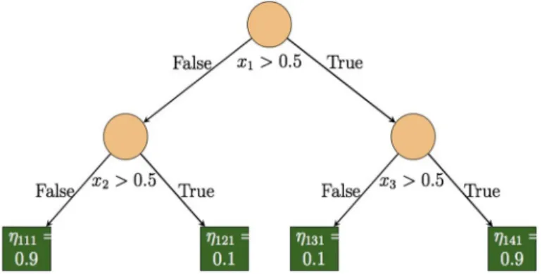
Fig. 2 One of the trees used in simulation Scenario 1 (Khan et al.2016)
3.1.1 Scenario 1
This scenario consists of 3 tree components each grown on 3 variables withT =3,
Z1=
3
t=1pˆt andXbecomes an×9 dimensional vector.
3.1.2 Scenario 2
In this scenario we take a total ofT = 4 trees whereZ2 =
4
t=1pˆt such thatX
becomes an×12 dimensional vector.
3.1.3 Scenario 3
This scenario is based on T = 5 trees such thatZ3 =
5
t=1pˆt andXbecomes a
n×15 dimensional vector.
3.1.4 Scenario 4
This scenario consists of 6 tree components which follows that,T =6,Z4=
6
t=1pˆt
andXbecomes an×18 dimensional vector.
To understand how the trees are grown in the above simulation scenarios, a tree
used in simulation Scenario 1 is given in Fig.2.
The values ofc1andc2are fixed at 0.5 and 15, respectively, in all the scenarios for
all variants. A total ofn =1000 observation are generated using the above setup.kNN,
CART, random forest, node harvest, SVM andOTEare trained by using 90% of the
data as training data (of which 90% is for bootstrapping and 10% for diversity check,
in the case ofOTE) and then applying the remaining 10% data as test data for testing
purpose. ForOTE,T = 1000 trees are grown as the initial ensemble. Experiments
are repeated 1000 times in each scenario giving a total of 1000 realizations. The final results are obtained by averaging outcomes under the 1000 realizations made in all the
scenarios and are given in Table2. Node weights are changed in a manner that could
make the patterns in the data less meaningful and thus getting a higher Bayes error.
Table 2 Classification error (in percent) of k NN, tree, random forest, node harv est, SVM and O TE Model dn Bayes error kNN T ree R F N H SVM (Radial) SVM (Linear) SVM (Bessel) SVM (Laplacian) O T E R eduction in E nsemble Size (%) [trees selected] Scenario 1 9 1000 9.0 2 2 9 .9 9.6 9 .8 19 19 19 19 9.5 89.8 [102] 14 26 15 15 15 22 22 23 22 15 89.8 [102] 17 32 18 18 21 28 28 28 28 18 89.8 [102] 33 42 36 35 36 37 37 38 37 37 89.8 [102] Scenario 2 1 2 1000 21 29 22 21 21 24 23 30 24 21 89.8 [102] 24 31 25 24 24 26 26 32 26 23 89.7 [103] 28 36 30 28 29 31 30 36 31 29 89.7 [103] 30 39 32 32 32 33 33 38 33 32 89.7 [103] Scenario 3 1 5 1000 15 31 22 18 22 24 24 55 24 18 89.8 [102] 18 32 24 21 24 26 25 55 26 22 89.5 [105] 21 34 25 23 27 27 27 55 27 24 89.5 [105] 24 36 29 28 29 29 29 54 30 28 89.5 [105] Scenario 4 1 8 1000 21 34 28 23 25 25 25 72 27 22 89.8 [102] 22 35 27 23 26 27 27 71 28 24 90.0 [100] 25 39 31 26 29 31 31 67 35 27 89.8 [102] 26 40 31 28 30 32 32 68 36 29 89.8 [102] The forth column of the table sho w s B ayes error for each model The last column is the percentage reduction (rounded to the nearest inte g er v alue) in the size of OT E compared to random forest where the number o f selected trees by OT E are g iv en in square brack ets
(a) (b) 0.0 0.2 0.4 0.6 0.8 1.0 Error Rate kNN Tre e RF NH
SVM_Rad SVM_Lin SVM_Bes SVM_Lap RP_LD
A RP_QD A OT E 0.0 0.2 0.4 0.6 0.8 1.0 Error Rate kNN Tre e RF NH
SVM_Rad SVM_Lin SVM_Bes SVM_Lap RP_LD
A RP_QD A OT E (c) (d) 0.0 0.2 0.4 0 .6 0.8 1.0 Error Rate kNN Tre e RF NH
SVM_Rad SVM_Lin SVM_Bes SVM_Lap RP_LD
A RP_QD A OT E 0.0 0.2 0.4 0 .6 0.8 1.0 Error Rate kNN Tre e RF NH
SVM_Rad SVM_Lin SVM_Bes SVM_Lap RP_LD
A
RP_QD
A
OT
E
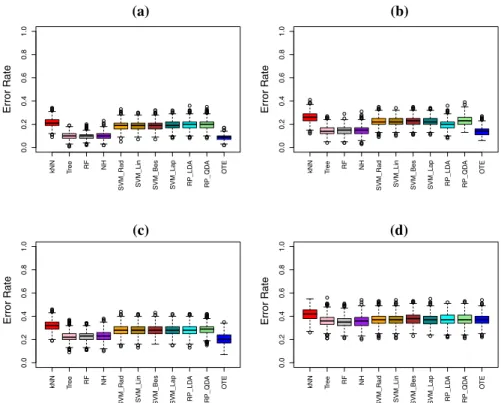
Fig. 3 Box plots forkNN, tree, random forest (RF), node harvest (NH), SVM andOTEon the data simulated
in Scenario 1.aSimulation with Bayes error 9%,bsimulation with Bayes error 14%,csimulation with
Bayes error 17% anddsimulation with Bayes error 33%. The best results ofOTEcan be seen in a where
the model produces a data with almost perfect tree structures.dThis shows the worst example ofOTE
different values of the Bayes error. It can be observed in the simulation that Bayes error of a scenario can be regulated by changing either the number of trees in the scenario
or node weights of the trees or both. For example, weights of 0.9 and 0.1 assigned to
extreme nodes (right most and left most) and inner nodes, respectively, would lead to
a less complex tree as compared to the one with 0.8 and 0.2 such weights. Tree given
in Fig.2is the least complex tree used in the simulation in terms of Bayes error. As
anticipated,kNN and tree classifiers have the highest percentage errors in all the four
scenarios. Random forest andOTEperformed quite similarly with slight variations
in few cases. In cases where the models have the highest Bayes error, the results of
random forest are better or comparable with those ofOTE. In all the remaing cases
where the Bayes error is the smallest,OTEis better or comparable with random forest.
SVM performed very similarly tokNN and tree. Percentage reduction in ensemble
size ofOTEcompared to random forest is also shown in the last column of the table.
A 90% reduction in the size would mean that OTEuse only 10 trees to achieve a
performance level of a random forest of 100 trees. This means thatOTEcould be very
helpful in decreasing the size of the ensemble thus reducing storage costs.
The box plots given in Fig.3reveal that the best results ofOTEcan be observed in
worst example ofOTEwhere the Bayes error is the highest (i.e. 33%), and where the data have no meaningful tree structures.
3.2 Benchmark problems
For assessing the performance ofOTEon benchmark problems, we have considered
35 data sets out of which 14 are regression and 21 classification problems. A brief
summary of the data sets is given in Table3. The upper portion of Table3are regression
problems whereas the lower portion are classification problems.
3.3 Experimental setup for benchmark data sets
Experiments carried out on the 35 data sets are designed as follows. Each data set is divided into two parts, a training part and testing part. The training part consists of 90% of the total data while the testing part consists of the remaining 10% of the
data. A total ofT =1500 independent classification and regression trees are grown on
bootstrap samples from 90% of training data along with randomly selectingpfeatures
for splitting the nodes of the trees. The remaining 10% of training data is used for
diversity check. In the cases of both regression and classification, the number p of
features is kept constant at p=√dfor all data sets. The best of the totalT trees are
selected by using the method given in Sect.2and are used as the final ensemble (M
is taken as 20% ofT). Testing part of the data is applied on the final ensemble and a
total of 1000 runs are carried out for each data set. Final result is the average of all these 1000 runs. The same setting is used for the optimal trees ensemble in Khan et al.
(2016) i.e. OTE.Prob.
For tuning various parameters of CART, we used the R-Function “tune.rpart”
avail-able within the R-Package “e1071” (Meyer et al.2014). We tried various values, (5,
10, 15, 20, 25, 30) for finding the optimal number of splits and the minimal optimal depth of the trees.
For tuning the hyper parameters,nodesize,ntreeandmtry of random forest, we
used the function “tune.randomForest” available with in the R-Package “e1071” as
used by Adler et al. (2008). For tuning the node size we tried values (1, 5, 10, 15, 20,
25, 30), for tuning ntree we tried values (500, 1000, 1500, 2000) and for tuning mtry, we tried (sqrt(d), d/5, d/4, d/3, d/2). We tried all the possible values of mtry where
d <12.
The only parameter in the node harvest estimator is the number of nodes in the
initial ensemble and for its large values the results are insensitive (Meinshausen2010).
Meinshausen (2010) showed for various data sets that initial ensemble size greater than
1000 yields almost the same results. In our experiments we kept this value fixed at 1500. In case of SVM, automatic estimation of sigma was used available with in the R package “kernlab”. The rest of the parameters are kept at default values. Four kernels,
Radial, Linear, Bessel and Laplacian, are used for SVM.kNN is tuned by using the R
function “tune.knn” within the R library “e1071” for various values of the number of
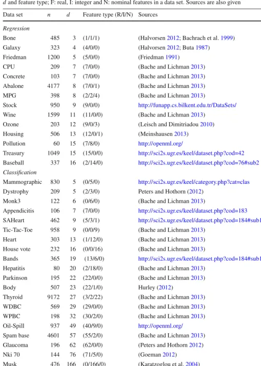
Table 3 Data sets for classification and regression with total number of observationsn, number of features dand feature type; F: real, I: integer and N: nominal features in a data set. Sources are also given
Data set n d Feature type (R/I/N) Sources
Regression
Bone 485 3 (1/1/1) (Halvorsen2012; Bachrach et al.1999)
Galaxy 323 4 (4/0/0) (Halvorsen2012; Buta1987)
Friedman 1200 5 (5/0/0) (Friedman1991)
CPU 209 7 (7/0/0) (Bache and Lichman2013)
Concrete 103 7 (7/0/0) (Bache and Lichman2013)
Abalone 4177 8 (7/0/1) (Bache and Lichman2013)
MPG 398 8 (2/2/4) (Bache and Lichman2013)
Stock 950 9 (9/0/0) http://funapp.cs.bilkent.edu.tr/DataSets/
Wine 1599 11 (11/0/0) (Bache and Lichman2013)
Ozone 203 12 (9/0/3) (Leisch and Dimitriadou2010)
Housing 506 13 (12/0/1) (Meinshausen2013) Pollution 60 15 (7/8/0) http://openml.org/ Treasury 1049 15 (15/0/0) http://sci2s.ugr.es/keel/dataset.php?cod=42 Baseball 337 16 (2/14/0) http://sci2s.ugr.es/keel/dataset.php?cod=76#sub2 Classification Mammographic 830 5 (0/5/0) http://sci2s.ugr.es/keel/category.php?cat=clas
Dystrophy 209 5 (2/3/0) Peters and Hothorn (2012)
Monk3 122 6 (0/6/0) (Bache and Lichman2013)
Appendicitis 106 7 (7/0/0) http://sci2s.ugr.es/keel/dataset.php?cod=183
SAHeart 462 9 (5/3/1) http://sci2s.ugr.es/keel/dataset.php?cod=184#sub1
Tic-Tac-Toe 958 9 (0/0/9) (Bache and Lichman2013)
Heart 303 13 (1/12/0) (Bache and Lichman2013)
House vote 232 16 (0/0/16) (Bache and Lichman2013)
Bands 365 19 (13/6/0) http://sci2s.ugr.es/keel/dataset.php?cod=184#sub1
Hepatitis 80 20 (2/18/0) (Bache and Lichman2013)
Parkinson 195 22 (22/0/0) (Bache and Lichman2013)
Body 507 23 (22/1/0) Hurley (2012)
Thyroid 9172 27 (3/2/22) (Bache and Lichman2013)
WDBC 569 29 (29/0/0) (Bache and Lichman2013)
WPBC 198 32 (30/2/0) (Bache and Lichman2013)
Oil-Spill 937 49 (40/9/0) http://openml.org/
Spam base 4601 57 (55/2/0) (Bache and Lichman2013)
Glaucoma 196 62 (62/0/0) (Peters and Hothorn2012)
Nki 70 144 76 (71/5/0) (Goeman2012)
A recently proposed method, random projection (RP) ensemble (Cannings and
Samworth 2017), has also been considered for comparison purposes using the
“RPEnsemble” (Cannings and Samworth 2016) R package. Due to computational
constraint we have used B1 = 30 and B2 = 5. Linear discriminant analysis
base = “LDA”and quadratic discriminant analysisbase = “QDA”methods are
used as the base classifiers along withd=5, projmethod = “Haar”keeping
the rest of the parameters at their default values. We did not usek-NN base as it has
been shown outperformed by LDA and QDA (Cannings and Samworth2017).
The same set of training and test data is used for tree, random forest, node harvest, SVM and our proposed method. Average unexplained variances and classification errors, for regression and classification respectively, are noted down for all the four methods on the data sets. All the experiments are done using R version 3.0.2 R Core
Team (2014). The results are given in Tables4and5for regression and classification
respectively.
3.4 Discussion
The results given in Tables4and5show that the proposed method is performing better
than the other methods on many of the data sets. In the case of regression problems, our method is giving better results than the other methods considered on 7 data sets out of a total of 14 data sets, whereas on 2 data sets, Wine and Abalone, random forest gives the best performance. On 5 of the data sets, Bone, Galaxy, Freidman, and Ozone, SVM with radial kernel and Concrete with Bessel kernel gave the best results. Tree
andkNN are unsurprisingly the worst performers in all the methods with the exception
of the Stock data set wherekNN is the best.
In the case of classification problems, the new method is giving better results than the other methods considered on 9 data sets out of a total of 21 data sets and comparable to random forest on 1 data set. On 3 data sets, random forest gives the best performance. On three of the data sets, Mammographic, Appendicitis and SAHeart, node harvest classifier gives the best result among all other methods. SVM is better than the others on 3 data sets. Random projection ensemble gave better results on 3 data set.
Moverover, the optimal trees ensemble in Khan et al. (2016), OTE.Prob, when
evaluated by classification error rates, is also giving very close results to those ofOTE.
This can be seen in the last two columns of Table5where the result of OTE.Prob is
itilicised when it performed better thanOTE.
Overall, the proposed method gave better results on 13 data sets and comparable results on 2 data set.
We kept all our parameters in the ensemble fixed for the sake of simplicity.
Search-ing for the optimal total numberT of trees grown before the selection process, the
percentage M of best trees selected at the first phase, node size and the number of
features for splitting the nodes might further improve our results. Large values are recommended for the size of the initial set under the available computation resources
and a value of T ≥ 1500 is expected to work well in general. This can be seen in
Fig.4that show the effect of the number of trees in the initial set on (a): unexplained
Table 4 Une xplained v ariances for re g ression data sets from k NN, tree, random forest, node harv est, SVM and OT E Data set nd k NN T ree RF NH SVM (Radial) SVM (Linear) SVM (Bessel) SVM (Laplacian) O TE Bone 485 3 0 .8932 0.7058 0.6601 0.6632 0.6292 0.7908 0.7369 0.6329 0.6454 Galaxy 323 4 0 .0285 0.0952 0.0275 0.0686 0.0253 0.1153 0.0356 0.0262 0.0261 Friedman 1200 5 0 .1373 0.3871 0.1212 0.4452 0.0559 0.2828 0.0849 0.0657 0.1364 CPU 209 7 0 .1058 0.2838 0.0646 0.2659 0.3898 0.0916 0.2861 0.3143 0.0600 Concrete 103 7 0 .3720 0.4989 0.2174 0.4307 0.0700 0.1743 0.0623 0.1806 0.2342 Abalone 4177 8 0 .5347 0.5673 0.4386 0.6083 0.4410 0.4904 0.4433 0.4418 0.4473 MPG 398 8 0 .3230 0.2301 0.1259 0.1990 0.1358 0.2066 0.1435 0.1359 0.1203 Stock 950 9 0.0102 0.0942 0.0121 0.1192 0.0153 0.1373 0.0274 0.0142 0.0110 W ine 1599 11 0.8975 0.7140 0.4933 0.7044 0.5980 0.6653 0.8991 0.5859 0.5072 Ozone 203 12 0.6430 0.4366 0.3061 0.3642 0.2488 0.3528 0.7967 0.2750 0.3016 Housing 506 13 0.4696 0.2821 0.1190 0.2477 0.1756 0.3055 0.8824 0.1853 0.1160 Pollution 6 0 1 5 0 .9500 0.9500 0.6779 0.7728 0.6942 0.8144 0.9500 0.7326 0.6653 T reasury 1049 15 0.0075 0.0405 0.0040 0.0574 0.0062 0.0060 0.0077 0.0070 0.0039 Baseball 337 16 0.6931 0.3513 0.3434 0.3908 0.3641 0.3818 0.8765 0.3641 0.3329 The une xplained v ariance of the b est p erforming m ethod for the corresponding data set is sho wn in bold
Table 5 Classification error rates of k NN, tree, random forest, node harv est, SVM, random projection w ith linear and quadractic discriminant analyses, OT E and O TE.Prob Khan et al. ( 2016 ) Data set nd k NN T ree RF NH SVM (Radial) SVM (Linear) SVM (Bessel) SVM (Laplacian) RP (LD A ) R P O TE (QD A ) O TE.Prob Mammographic 830 5 0 .1901 0.1631 0.1670 0.1579 0.1910 0.1750 0.1875 0.1863 0.1889 0.1957 0.1711 0 .1710 Dystrophy 209 5 0 .1172 0.1482 0.1154 0.1470 0.0999 0.1122 0.1070 0.0997 0.1206 0.0924 0.1182 0.1183 Monk3 122 6 0 .1226 0.0773 0.0728 0.2699 0.0953 0.2254 0.0928 0.0938 0.2024 0.1065 0.0731 0.0735 Appendicitis 106 7 0 .1423 0.1640 0.1455 0.1380 0.2245 0.1726 0.1905 0.1650 0.1818 0.1450 0.1500 0.1504 SAHeart 462 9 0 .3363 0.2911 0.2897 0.2762 0.3075 0.3080 0.3332 0.3139 0.3017 0.3033 0.3178 0.3177 T ic-T ac-T o e 958 9 0 .3617 0.1082 0.0317 0.2861 0.2078 0.3948 0.1725 0.1972 0.3002 0.2312 0.0353 0.0351 Heart 303 13 0.3500 0.2108 0.1629 0.1892 0.2342 0.1745 0.1612 0.1719 0.1666 0.1958 0.1743 0.1744 House V ote 232 16 0.0825 0.0345 0.0322 0.1020 0.0330 0.0470 0.2211 0.0529 0.0650 0.1454 0.0340 0.0344 Bands 365 19 0.3196 0.3683 0.2683 0.3647 0.3669 0.3202 0.4724 0.5573 0.3382 0.3144 0.2601 0.2602 Hepatitis 80 20 0.3831 0.1868 0.1385 0.1296 0.1406 0.1568 0.5629 0.1490 0.1921 0.1614 0.1229 0.1230 P arkinson 195 22 0.1620 0.1456 0.0894 0.1235 0.1385 0.1941 0.2838 0.1928 0.1844 0.1577 0.0859 0.0861 Body 507 23 0.0226 0.0788 0.0395 0.0744 0.0156 0.0136 0.5505 0.0219 0.0196 0.0234 0.0380 0.0371 Thyroid 9172 27 0.0388 0.0126 0.0100 0.0203 0.1113 0.0310 0.2936 0.0834 0.0503 0.0426 0.0100 0.0103 WDBC 569 29 0.0671 0.0686 0.0388 0.0525 0.0415 0.0264 0.6297 0.0403 0.0526 0.0568 0.0375 0.0374 WPBC 198 32 0.2413 0.2815 0.1958 0.2282 0.2848 0.2881 0.5684 0.3084 0.2631 0.2263 0.1921 0.1922 Oil-Spill 937 49 0.0435 0.0366 0.0330 0.0360 0.0756 0.1400 0.0387 0.1467 0.0444 0.0423 0.0321 0.0320 Spam base 4601 58 0.1747 0.1083 0.0469 0.0944 0.0941 0.0725 0.4820 0.1020 0.2162 0.3189 0.0460 0.0463 Sonar 208 60 0.1790 0.2879 0.1615 0.2390 0.1710 0.2505 0.5300 0.2698 0.4285 0.2058 0.1600 0.1616 Glaucoma 196 62 0.1934 0.1237 0.1052 0.1154 0.1108 0.1565 0.6397 0.1664 0.1008 0.1455 0.1051 0.1053 Nki 7 0 144 76 0.1827 0.1683 0.1466 0.1448 0.2664 0.3381 0.4260 0.4089 0.1773 0.1837 0.1399 0.1396 Musk 476 166 0.1420 0.2256 0.1103 0.2444 0.1326 0.1440 0.4964 0.4698 0.0957 0.0716 0.0949 0.0947 The result o f the best performing m ethod for the corresponding data set is sho wn in bold. The result o f O TE.Prob is italicised when it is better than OT E
(a) (b) 0 1000 2000 3000 4000 0.0 0 .2 0.4 0.6 0.8 1.0
Number of Trees in Initial Set
Une xplained V a riance Bone Galaxy Stock Ozone Housing Baseball 0 1000 2000 3000 4000 0.0 0 .1 0.2 0.3 0.4
Number of Trees in Initial Set
Error Rate Hepatitis Body Thyroid WDBC WPBC Glaucoma
Fig. 4 The effect of the number of trees in the initial set onaunexplained variance andb misclassifica-tion error for the data sets given usingOTE. In both the cases, number of trees larger than 1500 can be recommended (a) (b) 0 10 20 30 40 50 60 70 0.0 0 .1 0.2 0.3 0 .4 0.5 0.6 M (in Percentage) Une xplained V a riance Ozone Housing Treasury Baseball Concrete 0 10 20 30 40 50 60 70 0.00 0.05 0.10 0.15 0.20 0.25 0.30 0.35 M (in Percentage) Error Rate Mammographic Sonar Tic.Tac.Toe Monk3 WPBC
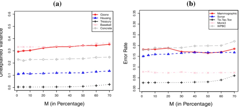
Fig. 5 Effect ofMon the unexplained variances (a) and error rate (b), of the data sets shown usingOTE. The value ofMin percentage is on the x-axis and unexplained variance on the y-axis
One important parameter of our method is the numberM of best trees selected at
the first phase for the final ensemble. Various values ofMreveal different behaviour of
the method. We considered the effect ofM =(1%,5%,10%,20%, . . . ,70%)of the
totalT trees on the method for both regression and classification as shown in Fig.5. It
is clear from Fig.5that the highest accuracy is obtained by using only a small portion,
1–10%, of the total trees that are individually strong which is further reduced in the second phase. This may significantly decrease the storage costs of the ensemble while increasing/without loosing accuracy. On the other hand, having a large number of trees may not only increase storage costs of the resulting ensemble but also decrease the
overall prediction accuracy of the ensemble. This can be seen in Fig.5in the cases of
Concrete, WPBC and Ozone data sets where the best results are obtained at about less than 5% best trees of the total trees at the first phase. This might be due to the reason that in such cases the possibility of having poor trees is high if the size of ensemble is
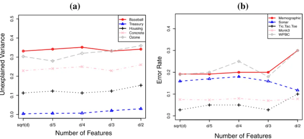
0.0 0 .1 0.2 0 .3 0.4 0 .5 Number of Features Une x plained V a riance Baseball Treasury Housing Concrete Ozone sqrt(d) d/5 d/4 d/3 d/2 0.0 0 .1 0.2 0.3 0.4 Number of Features Error Rate Memographic Sonar Tic.Tac.Toe Monk3 WPBC sqrt(d) d/5 d/4 d/3 d/2 (a) (b)
Fig. 6 Effect of the number of features (on x-axis) selected at random for splitting the nodes of the trees on the unexplained variance (a), and error rate (b) for the data sets shown usingOTE
large and trees are simply grown with out considering their individual and collective behaviours.
We also looked at the effect of various numbers p = √d,d5,d4,d3,d2 of features
selected at random for splitting the nodes of the trees on the unexplained variances and classification error in the cases of both regression and classification, respectively,
for some data sets. The graph is shown in Fig.6. The only reason that random forest is
considered as an improvement over bagging is the inclusion of additional randomness by randomly selecting a subset of features for splitting the nodes of the tree. The effect
of this randomness can be seen in Fig.6where different values ofpresults in different
unexplained variances/classification errors for the data sets. For example in the case
of Ozone data, selecting a higher value of padversely affects the performance. For
some data sets, Sonar for example, selecting largepresults in better performance.
4 Conclusion
The possibility of selecting best trees from an original ensemble of a large number of trees, and combining them together to vote/average for the response is considered. The new method is applied on 35 data sets consisting of 14 regression problems and
21 classification problems. The ensemble performed better thankNN, tree, random
forest, node harvest and SVM on many of the data sets. The intuition for the better performance of the new method is that if the base learners in the ensemble are individ-ually accurate and diverse, then their ensemble must give better or at least comparable results as compared to the one consisting of all weak learners. This might also be due to the reason that there could be various different meaningful structures present in the data that could not be captured by an ordinary algorithm. Our method tries to find these meaningful structures in the data and ignore those that only increase the error.
Our simulation reveals that the method can find meaningful patterns in the data as effectively as other complex methods might do.
Even if one could get comparable results by using a few strong and diverse base learners to those based upon thousands of weak base learners should be welcomed. This might be very helpful in reducing the associated storage costs of tree forests with little or no loss of prediction accuracy.
The method is implemented in the R-Package “OTE” (Khan et al.2014).
A practical challenge for OTE arises when we have relatively small number of
observations in the data. The trees are grown on 90% of the training data leaving the remaing 10% for internal validation. This might result in missing some important
information to learn from while traingOTE. On the other hand, the rest of the methods
use the whole training data. Solving this issue might further improve the results of
OTE. One way to solve this issue could be using the out-of-bag data from boostrap
samples again in a clever way while adding the corresponding trees for collective performance.
The use of some variable selection methods, (Hapfelmeier and Ulm2013; Mahmoud
et al.2014a,b; Brahim and Limam2017; Janitza et al.2015), might, in conjunction
with our method, lead to further improvements. Using the idea of random projection
ensembles (Cannings and Samworth2016,2017) with the proposed method may also
allow further improvements.
Acknowledgements We acknowledge support from grant number ES/L011859/1, from The Business and Local Government Data Research Centre, funded by the Economic and Social Research Council, UK, to provide researchers and analysts with secure data services.
Open Access This article is distributed under the terms of the Creative Commons Attribution 4.0 Interna-tional License (http://creativecommons.org/licenses/by/4.0/), which permits unrestricted use, distribution, and reproduction in any medium, provided you give appropriate credit to the original author(s) and the source, provide a link to the Creative Commons license, and indicate if changes were made.
References
Adler W, Peters A, Lausen B (2008) Comparison of classifiers applied to confocal scanning laser ophthal-moscopy data. Methods Inf Med 47(1):38–46
Adler W, Gefeller O, Gul A, Horn FK, Khan Z, Lausen B (2016) Ensemble pruning for glaucoma detection in an unbalanced data set. Methods Inf Med 55(6):557–563
Ali K, Pazzani M (1996) Error reduction through learning multiple descriptions. Mach Learn 24(3):173–202
Bache K, Lichman M (2013) UCI machine learning repository.http://archive.ics.uci.edu/ml
Bachrach LK, Hastie T, Wang MC, Narasimhan B, Marcus R (1999) Bone mineral acquisition in healthy asian, hispanic, black, and caucasian youth: a longitudinal study. J Clin Endocrinol Metab 84(12):4702– 4712
Bauer E, Kohavi R (1999) An empirical comparison of voting classification algorithms: bagging, boosting, and variants. Mach Learn 36(1):105–139
Bernard S, Heutte L, Adam S (2009) On the selection of decision trees in random forests. In: International joint conference on neural networks, IEEE, pp 302–307
Bhardwaj M, Bhatnagar V, Sharma K (2016) Cost-effectiveness of classification ensembles. Pattern Recognit 57:84–96
Bolón-Canedo V, Sánchez-Maroño N, Alonso-Betanzos A (2012) An ensemble of filters and classifiers for microarray data classification. Pattern Recognit 45(1):531–539
Brahim AB, Limam M (2017) Ensemble feature selection for high dimensional data: a new method and a comparative study. Adv Data Anal Classif 12:1–16
Breiman L (2001) Random forests. Mach Learn 45(1):5–32
Buta R (1987) The structure and dynamics of ringed galaxies. iii-surface photometry and kinematics of the ringed nonbarred spiral ngc 7531. Astrophys J Suppl Ser 64:1–37
Cannings TI, Samworth RJ (2016) RPEnsemble: Random Projection Ensemble Classification.https://
CRAN.R-project.org/package=RPEnsemble, r package version 0.3
Cannings TI, Samworth RJ (2017) Random-projection ensemble classification. J R Stat Soc Ser B (Stat Methodol) 79(4):959–1035
Domingos P (1996) Using partitioning to speed up specific-to-general rule induction. In: Proceedings of the AAAI-96 workshop on integrating multiple learned models, Citeseer, pp 29–34
Friedman JH (1991) Multivariate adaptive regression splines. Ann Stat 19:1–67
Goeman JJ (2012) penalized: Penalized generalized linear models. http://CRAN.R-project.org/
package=penalized, penalized R package, version 0.9-42
Gul A, Khan Z, Perperoglou A, Mahmoud O, Miftahuddin M, Adler W, Lausen B (2016a) Ensemble of subset of k-nearest neighbours models for class membership probability estimation. In: Analysis of large and complex data, Springer, pp 411–421
Gul A, Perperoglou A, Khan Z, Mahmoud O, Miftahuddin M, Adler W, Lausen B (2016b) Ensemble of a subset of knn classifiers. Adv Data Anal Classif 12:1–14
Halvorsen K (2012) ElemStatLearn: Data sets, functions and examples.http://CRAN.R-project.org/
package=ElemStatLearn, r package version 2012.04-0
Hapfelmeier A, Ulm K (2013) A new variable selection approach using random forests. Comput Stat Data Anal 60:50–69.https://doi.org/10.1016/j.csda.2012.09.020
Hothorn T, Lausen B (2003) Double-bagging: combining classifiers by bootstrap aggregation. Pattern Recognit 36(6):1303–1309
Hurley C (2012) gclus: Clustering Graphics.http://CRAN.R-project.org/package=gclus, r package version 1.3.1
Janitza S, Celik E, Boulesteix AL (2015) A computationally fast variable importance test for random forests for high-dimensional data. Adv Data Anal Classif 12:1–31
Karatzoglou A, Smola A, Hornik K, Zeileis A (2004) kernlab—an S4 package for kernel methods in R. Journal of Statistical Software 11(9):1–20,http://www.jstatsoft.org/v11/i09/
Khan Z, Gul A, Perperoglou A, Mahmoud O, Werner Adler M, Lausen B (2014) OTE: Optimal Trees Ensembles.https://cran.r-project.org/package=OTE, r package version 1.0
Khan Z, Gul A, Mahmoud O, Miftahuddin M, Perperoglou A, Adler W, Lausen B (2016) An ensemble of optimal trees for class membership probability estimation. In: Analysis of large and complex data, Springer, pp 395–409
Latinne P, Debeir O, Decaestecker C (2001a) Limiting the number of trees in random forests. In: Multi-ple Classifier Systems: Second International Workshop, MCS 2001 Cambridge, UK, July 2-4, 2001 Proceedings, Springer Science & Business Media, vol 2, p 178
Latinne P, Debeir O, Decaestecker C (2001b) Limiting the number of trees in random forests. Multiple Classifier Systems pp 178–187
Lausser L, Schmid F, Schirra LR, Wilhelm AF, Kestler HA (2016) Rank-based classifiers for extremely high-dimensional gene expression data. Adv Data Anal Classif 12:1–20
Leisch F, Dimitriadou E (2010) mlbench: Machine learning benchmark problems. R package version 2.1-1 Li HB, Wang W, Ding HW, Dong J (2010) Trees weighting random forest method for classifying high-dimensional noisy data. In: IEEE 7th international conference on e-business engineering (ICEBE), 2010, IEEE, pp 160–163
Liberati C, Camillo F, Saporta G (2017) Advances in credit scoring: combining performance and interpre-tation in kernel discriminant analysis. Adv Data Anal Classif 11(1):121–138
Maclin R, Opitz D (2011) Popular ensemble methods: an empirical study. J Artif Res 11:169–189 Mahmoud O, Harrison A, Perperoglou A, Gul A, Khan Z, Lausen B (2014a) propOverlap:
Fea-ture (gene) selection based on the Proportional Overlapping Scores.http://CRAN.R-project.org/
package=propOverlap, r package version 1.0
Mahmoud O, Harrison A, Perperoglou A, Gul A, Khan Z, Metodiev MV, Lausen B (2014b) A feature selection method for classification within functional genomics experiments based on the proportional overlapping score. BMC Bioinf 15(1):274
Meinshausen N (2010) Node harvest. Ann Appl Stat 4(4):2049–2072
Meinshausen N (2013) nodeHarvest: Node Harvest for regression and classification.
Meyer D, Dimitriadou E, Hornik K, Weingessel A, Leisch F (2014) e1071: Misc Functions of the Department of Statistics (e1071), TU Wien.http://CRAN.R-project.org/package=e1071, r package version 1.6-4 Mitchell T (1997) Machine learning. McGraw Hill, Burr Ridge
Oshiro T, Perez P, Baranauskas J (2012) How many trees in a random forest? Machine Learning and Data Mining in Pattern Recognition, pp 154–168
Peters A, Hothorn T (2012) ipred: Improved predictors.http://CRAN.R-project.org/package=ipred, r pack-age version 0.9-1
Quinlan J (1996) Bagging, boosting, and c4. 5. In: Proceedings of the national conference on artificial intelligence, pp 725–730
R Core Team (2014) R: A language and environment for statistical computing. R Foundation for Statistical
Computing, Vienna, Austria,http://www.R-project.org/
Schapire R (1990) The strength of weak learnability. Mach Learn 5(2):197–227
Tumer K, Ghosh J (1996) Error correlation and error reduction in ensemble classifiers. Connect Sci 8(3– 4):385–404
Tzirakis P, Tjortjis C (2017) T3c: improving a decision tree classification algorithm’s interval splits on continuous attributes. Adv Data Anal Classif 11(2):353–370
Zhang H, Wang M (2009) Search for the smallest random forest. Stat Interface 2(3):381–388
Publisher’s Note Springer Nature remains neutral with regard to jurisdictional claims in published maps and institutional affiliations.
Affiliations
Zardad Khan1,2·Asma Gul2,3·Aris Perperoglou2·
Miftahuddin Miftahuddin2,4·Osama Mahmoud2,5,6·Werner Adler7· Berthold Lausen2
1 Department of Statistics, Abdul Wali Khan University, Mardan, Pakistan
2 Department of Mathematical Sciences, University of Essex, Colchester CO4 3SQ, UK
3 Department of Statististics, Shaheed Benazir Bhutto Women University, Peshawar, Pakistan
4 College of Science, Syiah Kuala University, Banda Aceh, Indonesia
5 Department of Applied Statistics, Helwan University, Cairo, Egypt
6 School of Social and Community Medicine, University of Bristol, Bristol BS8 2BN, UK
7 Department of Biometry and Epidemiology, University of Erlangen-Nuremberg, Erlangen,