DEEP SEQUENTIAL AND STRUCTURAL
NEURAL MODELS OF COMPOSITIONALITY
A Dissertation
Presented to the Faculty of the Graduate School of Cornell University
in Partial Fulfillment of the Requirements for the Degree of Doctor of Philosophy
by Ozan ˙Irsoy January 2017
c
2017 Ozan ˙Irsoy
DEEP SEQUENTIAL AND STRUCTURAL NEURAL MODELS OF COMPOSITIONALITY
Ozan ˙Irsoy, Ph.D. Cornell University 2017
Recent advances in deep learning have provided fruitful applications for nat-ural language processing (NLP) tasks. One key advance was the invention of word vectors, representing every word in a dense, low-dimensional vector space. Even though word vectors provide very strong results for word level NLP tasks, producing appropriate representation for phrases and sentences is still an open research problem.
In this dissertation, we focus on compositional approaches to representation learning. In particular, we employ the notions of compositionality in which the sequence or structure information is utilized, via recurrent or recursive neu-ral networks. We investigate the effectiveness of such approaches for specific natural language understanding tasks including opinion mining and sentiment analysis, and extend some of the approaches to provide better representation hi-erarchies. In particular, we propose two novel variants: bidirectional recursive neural networks, which are capable of producing context-dependent structural representations and deep recursive neural networks, which provide represen-tation hierarchies in the structural setting. Additionally, we qualitatively inves-tigate such models, and describe how they relate to alternative compositional approaches. Finally, we discuss challenges in interpretation and understand-ing of compositional neural models, propose simple tools for visualization, and perform exploratory analyses over features learned by such a model.
BIOGRAPHICAL SKETCH
Ozan ˙Irsoy was born in ˙Izmir, Turkey. He pursued his Bachelor’s degrees in Mathematics and Computer Engineering at Bo˘gazic¸i University. During his un-dergraduate studies, he developed an interest in machine learning. His early work on decision trees that started as part of his Bachelor’s Thesis turned into several novel decision tree methods. Upon graduation, he has won several awards including Bo˘gazic¸i University Department of Computer Engineering and the School of Engineering Valedictorian, Double Major Graduate Award, and Best Bachelor’s Thesis Award.
After completion of the Bachelor’s degrees, he joined to Cornell University to pursue a doctorate degree in Computer Science. During his PhD, his research lied at the intersection of representation learning and natural language process-ing. He worked on learning (possibly deep) representations for composition-ality in language, with applications to sentiment analysis, opinion mining and question answering. He has completed internships at Google and MetaMind applying neural networks to natural language understanding and speech recog-nition problems.
ACKNOWLEDGEMENTS
I am extremely thankful to my advisor Claire Cardie for her infinite guidance, support, mentorship, suggestions, ideas and all the help she provided. I am also very grateful to my committee members Robert Kleinberg and Dawn Woodard for their insightful input and feedback to my research.
I would like to thank my mentors who inspired and helped me during my internships, Andrew Senior and Hasim Sak from Google and Richard Socher from MetaMind. Special thanks to Volkan Cirik, Ainur Yessenalina, and Bishan Yang for helping with some of the experiments in this thesis, and Mohit Iyyer for insightful discussions.
Many thanks to Moontae Lee, Vlad Niculae, Arzoo Katiyar, Bishan Yang, Lu Wang, Jon Park, Adith Swaminathan, Jason Yosinski, Lillian Lee, David Mimno, and all the members of the NLP Seminar and MLDG for their helpful feedback. I would like to thank my collaborator and Bachelor’s thesis advisor Ethem Alpaydın for introducing me to machine learning and artificial intelligence.
I thank my beautiful wife Gizem, for being the source of love, happiness, joy and strength.
TABLE OF CONTENTS
Biographical Sketch . . . iii
Dedication . . . iv Acknowledgements . . . v Table of Contents . . . vi List of Tables . . . ix List of Figures . . . x Notation . . . xii 1 Introduction 1 1.1 Overview . . . 1
1.1.1 Distributed Word Representations . . . 2
1.1.2 Composition of Word Vectors . . . 4
1.1.3 Artificial Neural Networks . . . 5
1.2 Contributions . . . 7
1.3 Roadmap . . . 8
2 Background and Related Work 10 2.1 Representation Learning . . . 10
2.2 Learning Word Representations . . . 11
2.3 Learning Representations for Phrases and Sentences . . . 13
2.3.1 Orderless Composition . . . 14
2.3.2 Sequential Composition . . . 15
2.3.3 Structural Composition . . . 18
3 Opinion Mining with Deep Recurrent Neural Networks 20 3.1 Related Work . . . 22
3.2 Sequential Neural Models for Opinion Mining . . . 23
3.2.1 Recurrent Neural Networks . . . 23
3.2.2 Bidirectionality . . . 25
3.2.3 Depth in Space . . . 27
3.3 Experiments . . . 29
3.3.1 Hypotheses . . . 29
3.3.2 Experimental Setting . . . 29
3.3.3 Results and Discussion . . . 32
3.4 Chapter Summary . . . 38
4 Modeling Compositionality with Multiplicative Recurrent Neural Networks 39 4.1 Related Work . . . 41
4.2 Composition with Matrix-Space Models . . . 43
4.3 Composition with Multiplicative Recurrent Neural Networks . . 44
4.3.2 Relationship to matrix-space model . . . 46
4.4 Experiments . . . 49
4.4.1 Experimental Setting . . . 49
4.4.2 Results and Discussion . . . 50
4.5 Chapter Summary . . . 53
5 Bidirectional Recursive Neural Networks for Token-Level Labeling with Structure 55 5.1 Related Work . . . 57
5.2 Structural Composition with Recursive Neural Networks . . . 58
5.3 Bidirectional Recursive Neural Networks . . . 60
5.3.1 Incorporating Sequential Context . . . 62
5.4 Experiments . . . 63
5.4.1 Experimental Setting . . . 63
5.4.2 Results and Discussion . . . 65
5.5 Chapter Summary . . . 68
6 Deep Recursive Neural Networks for Compositionality in Language 70 6.1 Related Work . . . 72
6.2 Deep Recursive Composition . . . 73
6.2.1 Untying Leaves and Internals . . . 74
6.2.2 Deep Recursive Neural Networks . . . 75
6.3 Experiments . . . 77
6.3.1 Experimental Setting . . . 77
6.3.2 Results and Discussion . . . 80
6.4 Chapter Summary . . . 85
7 Towards Understanding Neural Language Learners 87 7.1 Related Work . . . 88
7.2 Identifying Challenges . . . 90
7.3 Visualizing Hidden Features . . . 93
7.3.1 First Order Saliency and Expected Deviation . . . 95
7.3.2 Cross-Feature First Order Saliency . . . 97
7.3.3 Immediate Temporal Differences . . . 98
7.3.4 Fine-grained Activation Statistics . . . 99
7.4 Experiments . . . 100
7.4.1 Experimental Setting . . . 100
7.4.2 Results and Discussion . . . 102
7.5 Chapter Summary . . . 115
8 Conclusion and Future Work 119 8.1 Summary of Contributions . . . 119
A Additional Visualizations of Model Activations 123
A.1 Cross-feature Saliency . . . 123 A.2 Generic Sentiment Features . . . 124 A.3 Decorrelated Features . . . 125
LIST OF TABLES
3.1 An example sentence with opinion expression labels . . . 21 3.2 Experimental evaluation of recurrent networks for DSE extraction 32 3.3 Experimental evaluation of recurrent networks for ESE extraction 33 3.4 Comparison of Deep recurrent networks to state-of-the-art
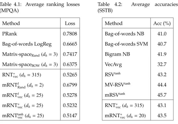
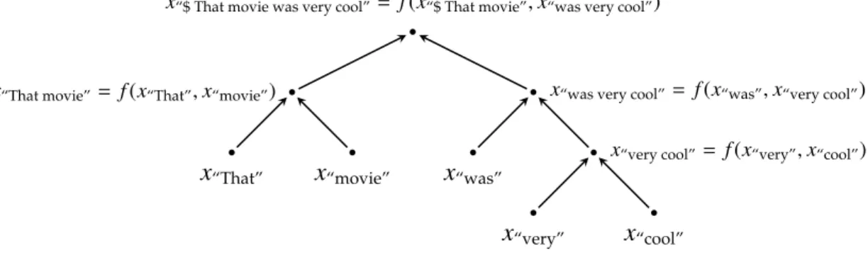
(semi)CRF baselines for DSE and ESE detection . . . 33 4.1 Average ranking losses (MPQA) . . . 52 4.2 Average accuracies (SSTB) . . . 52 5.1 An example sentence with opinion expression, holder, and target
labels . . . 57 5.2 Experimental results for DSE detection . . . 65 5.3 Experimental results for ESE detection . . . 65 5.4 Experimental results for joint HOLDER+DSE+TARGET detection 65 6.1 Results for RSVs. ` and |h| denote the depth and width of the
networks, respectively. . . 80 6.2 Results for previous work and our best model (dRSV). . . 81 6.3 Example shortest phrases and their nearest neighbors across
three layers. . . 84 7.1 Top activators of feature 4. Maximum activating words are
shown in boldface. . . 103 7.2 Highest activating words of(W x)4(top) and(Wzx)4(bottom).
Ac-tivation amounts are given in parentheses. . . 106 7.3 Lowest activators of feature 9. Activations are coded with
un-derline colors. . . 109 7.4 Highest activators of feature 2 after PCA. Activations are coded
with underline colors. . . 115 7.5 Highest activators of feature 4 after PCA. Activations are coded
with underline colors. . . 116 7.6 Top negative activators of feature 7 after PCA. Activations are
coded with underline colors. . . 117 A.1 Top activators of feature 5. Activations are coded with underline
colors. . . 125 A.2 Top activators of feature 14. Activations are coded with
under-line colors. . . 127 A.3 Top negative activators of feature 5 after PCA. Activations are
coded with underline colors. . . 127 A.4 Top activators of feature 7 after PCA. Activations are coded with
underline colors. . . 128 A.5 Top activators of feature 10 after PCA. Activations are coded
LIST OF FIGURES
1.1 Distributed word representations . . . 3 3.1 Recurrent neural networks. Each black, orange and red node
de-notes an input, hidden or output layer, respectively. Solid and dotted lines denote the connections of forward and backward layers, respectively. Top: Shallow unidirectional (left) and bidi-rectional (right) recurrent net. Bottom: 3-layer deep unidirec-tional (left) and bidirecunidirec-tional (right) recurrent net. . . 24 3.2 Examples of output. In each set, the gold-standard annotations
are shown in the first line. . . 36 3.3 DEEPRecurrent Output vs. SHALLOWRecurrent Output. In each
set of examples, the gold-standard annotations are shown in the first line. Tokens assigned a label of Inside with no preceding Begin tag are shown in ALL CAPS. . . 37 4.1 Vector x(blue) and tensorA(red) sliced along the dimension of
x. Left. Dense word vector x computes a weighted sum over
base matrices to get a square matrix, which then is used to trans-form the meaning vector. Right.One-hot word vector xwith the
same computation, which is equivalent to selecting one of the base matrices and falls back to a matrix-space model. . . 48 4.2 Hidden layer vectors reduced to 2 dimensions for various
phrases. Left. Recurrent neural network. Right. Purely
mul-tiplicative recurrent neural tensor network. In mRNT, handling of negation is more nonlinear and correctly shifts the sentiment. 51 5.1 Structural recursive composition . . . 56 5.2 Left. Recursive neural network with bottom-up propagation.
Right. Bidirectional recursive neural network with
bottom-up and top-down propagation. Black, orange and red denote bottom-up, top-down and output layers, respectively. Connec-tions that share the same color and style are shared. . . 59 5.3 Experimental results for joint detection over sentences with
sep-aration . . . 68 6.1 Operation of a recursive net (left), untied recursive net (middle)
and a recurrent net (right) on an example sentence. Black, orange and red dots represent input, hidden and output layers, respec-tively. Directed edges having the same color-style combination denote shared connections. . . 73
6.2 Operation of a 3-layerdeep recursive neural network. Red and
black points denote output and input vectors, respectively; other colors denote intermediate memory representations. Connec-tions denoted by the same color-style combination are shared
(i.e. share the same set of weights). . . 75
6.3 An example sentence with its parse tree (left) and the response measure of every layer (right) in a three-layered deep recur-sive net. We change the word “best” in the input to one of the words “coolest”, “good”, “average”, “bad”, “worst” (denoted by blue, light blue, black, orange and red, respectively) and mea-sure the change of hidden layer representations in one-norm for every node in the path. . . 83
7.1 Feature activators in computer vision and in NLP.Left. Highest activating image patches of a hidden unit of a single layer per-ceptron autoencoder. We can easily see the common pattern be-ing edge-like (actual values for the splittbe-ing hyperplane shown below). Right. Highest activating sentences of a hidden unit of a recurrent net. . . 92
7.2 Some high activators of feature 4. . . 104
7.3 More high activators of feature 4. . . 105
7.4 Top two activators of feature 9. . . 107
7.5 Some low activators of feature 7. . . 108
7.6 Some instances that have high output deviation with the absence of feature 7. . . 110
7.7 Some aggregate statistics of 25 features. Top. Mean average im-mediate squared change (spikyness). Middle.Mean average up-date gate activation. Bottom. Mean average squared activation (squared distance to zero). . . 111
7.8 Some instances that have high activation of feature 17. Saliency and expected deviations differ. . . 112
7.9 Some instances that have high activation of feature 18. Saliency and expected deviations differ. . . 113
A.1 Some activations visualized with cross-feature saliency values (second block of columns). Most values are close to zero. . . 123
A.2 More activations visualized with cross-feature saliency values (second block of columns). Values are away from zero. . . 124
NOTATION
|x| Dimensionality of vector x
|S| Cardinality of setS
[X,Y] Horizontal concatenation of blocksXandY
[X;Y] Vertical concatenation of blocksXandY 1(·) Indicator function
I(·) Identity function
I Identity matrix
R,Rn,Rm×n Set of real numbers, ndimensional real vectors, and mbyn real
valued matrices, respectively
A[i] ith slice of a third order tensorAofd
1×d2×d3(which is ad2×d3
matrix)
x,h,b,c Scalars or (column) vectors
W,V,U, A Matrices or higher order tensors
X,H,V,U,S Vector spaces, sets or probability distributions
f(·,·) Composition function
σ(·) Nonlinearity of hidden layers in a neural network γ(·) Nonlinearity of output layers in a neural network
t Index of an element in a sequence
CHAPTER 1
INTRODUCTION
1.1
Overview
Recent advances in neural networks and deep learning have provided fruit-ful applications for natural language processing (NLP) tasks. Neural networks employ representation and feature learning, as opposed to feature engineering which is traditionally used in NLP (Manning et al., 2008). Such representation learning approaches reached new state-of-the-art on many problems in NLP, such as language modeling (Mikolov et al., 2011), sentiment analysis (Socher et al., 2013), machine translation (Cho et al., 2014) and others. Furthermore, these approaches remove the necessity of manual feature engineering which is often laborious and time consuming.
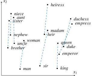
One especially important advance was the invention of word vector repre-sentations (Bengio et al., 2001). Word vectors represent every word in a dense, low dimensional space (see Figure 1.1), as opposed to traditional one-hot rep-resentation approach in which a word is assigned a vector of all zero values except a single one pointing to its index, which yields a sparse, high dimen-sional space. This representation also allows quantifying the similarity of dif-ferent words, using the notion of distance. In turn, word vector representations have been employed in many applications of deep learning in NLP, as the main atomic unit to represent text (Collobert and Weston, 2008; Collobert et al., 2011). Having strong tools for word representations, the natural next question, then, was how to properly map larger phrases into such dense representations
for NLP tasks that require properly capturing their meaning. Most existing methods take a compositional approach by defining a function that composes multiple word vector representations into representations of larger units of text, such as phrases or sentences (Mikolov et al., 2013b; Socher et al., 2013; Yesse-nalina and Cardie, 2011). These methods include orderless composition (simi-lar to how bag-of-words combines one-hot word representations) (Mitchell and Lapata, 2010; Zanzotto et al., 2010; Mikolov et al., 2013b; Iyyer et al., 2015), se-quential composition which combines words one-by-one in order (Rudolph and Giesbrecht, 2010; Yessenalina and Cardie, 2011; Mikolov et al., 2011) and struc-tural composition, which combines words into larger and larger phrases in a bottom-up fashion, using dependency or constituency parse trees (Socher et al., 2011b, 2012b, 2013), among others.
My research goal in this dissertation is to investigate and improve such compositional approaches, particularly sequential and structural approaches to compositionality.
1.1.1
Distributed Word Representations
In this dissertation, word vectors constitute the main building blocks of lan-guage. Word vectors represent a word as a point in a dense, continuous, low-dimensional (typically on the order of 100s) vector space. This is in contrast to the traditional approach of representing a word as a one-hot vector, which yields a sparse and very high dimensional (as many as the total number of words in the dictionary) representation. Additionally, dense word vectors provide a means to measure similarity between different words using the notion of distance (or
brother sister nephew niece uncle aunt man woman sir madam heir heiress king queen emperor empress duke duchess x1 x2
Figure 1.1: Distributed word representations
angle) whereas in one-hot word vectors every word has the same distance to every other word.
Word vectors are typically learned in an unsupervised fashion, which means we can employ large, unlabeled data sets for learning. Supervised approaches exist as well but they often do not have the benefit of having arbitrarily large data sets. Thus, in general, it is preferred to learn word vectors without super-vision and then fine-tune them for the supervised task at hand.
Word vectors have been shown to be good semantic representation of words, on many tasks (Mikolov et al., 2013b; Socher et al., 2011b; Collobert et al., 2011; Iyyer et al., 2015). Additionally, word vector spaces have been shown to have interestic geometric properties connected to their relationships (Mikolov et al., 2013a,b; Levy and Goldberg, 2014a). For instance, in Figure 1.1, transition from male to female nouns occur roughly along the same vector of translation. These results and attractive properties of word vectors have let them to achieve widespread use in the NLP community (Socher et al., 2012a).
1.1.2
Composition of Word Vectors
Having a mechanism for representing words, the next stage is to represent phrases or sentences, which is the main focus of this thesis.
Compositional approaches to semantic interpretation state that the meaning of a phrase, or sentence is a composition of the meaning of its parts. This, in the context of word vectors, could be interpreted as a unit of text being represented by some function of its word vectors. This naturally brings us to the question of what compositional function to use to combine word vectors to represent the meaning of phrases or sentences.
A simple way to combine word vectors in a phrase, or sentence is to just use a commutative (orderless) operation, such as elementwise multiplication or averaging. This alone has been shown to be effective in certain applications such as sentiment analysis even though the order information is lost (Mikolov et al., 2013b; Iyyer et al., 2015).
Alternatively, we might define a composition function that is respectful of the order. For instance, we might define a recursive function that starts from the first word vector and combines it with the second word vector, then combines the result with the third word vector, and so on until the last.
Such a recursive approach could also be applied over structural information, in particular, parse trees of sentences. We can apply the function recursively, in a bottom up fashion, to get vector representations of phrases and sentences from the representations of their children.
for composition are modeled by neural networks.
1.1.3
Artificial Neural Networks
The main building block of a neural network is the perceptron: the applica-tion of a (typically sigmoidal) nonlinearity funcapplica-tion on an affine transformaapplica-tion of the input. Deep neural networks involve cascading such perceptron layers, which allow multi-stage, hierarchical information processing through interme-diate representations of the input.
Some of the advantages of neural networks over alternative learners are: 1. Simplicity. Many different architectures can be defined using the same
building block and same formulation, all of which can be learned with the same algorithmic principle (backpropagation).
2. Effectiveness. Recent advances in computing power have resulted in the ability to train powerful neural networks that reached new state-of-the-art performance on many tasks ranging from computer vision to speech recognition.
3. Feature learning. Hierarchical representation learning in neural networks has shown the ability to combine simpler features into more and more complex and abstract features. In many cases, neural networks have elim-inated the need to do manual feature engineering (Krizhevsky et al., 2012; Le et al., 2012).
1. Black-box nature. Although neural networks may have good perfor-mance, they are essentially black-box learners and usually difficult to in-terpret. This inability to manually inspect the function that is realized by the network makes error analysis difficult. Thus, in applications where manual inspection of the prediction by an expert is necessary, such as med-ical diagnosis, they become unsuitable. Lack of interpretability holds in the case of NLP as well, relative to fields such as computer vision, where features have visual meaning and are easy to visually inspect.
2. Data size requirements. Purely supervised training of neural networks usually requires large data sets, typically at least around the order of 1000s-10000s of training examples. That makes neural networks difficult to apply to tasks where annotated data, i.e. text paired with supervisory labels, is not so abundant, which is not uncommon in NLP.
3. Soft computing. The continuous representations employed by neural net-works make them difficult to couple with symbolic, discrete approaches. Many problems in NLP are naturally formulated as discrete optimization problems which make neural networks difficult to apply, if not totally un-suitable.
This dissertation builds on top of existing neural network approaches that rely on sequential or structural interpretations of language. We investigate the effectiveness of such approaches for specific tasks of natural language under-standing, and extend some of the approaches to provide representation hier-archies. We aim to successfully represent meaning both in isolation, and in context, depending on the requirements of the application. In part, we unify matrix-space models, which is another distributed compositional model with-out word vectors, with the recurrent neural network approach.
1.2
Contributions
The primary contribution of this dissertation is the development and investiga-tion of effective models for representainvestiga-tion learning for composiinvestiga-tional meaning in natural language. More specifically, we make the following contributions:
Opinion mining without features using deep sequential models. We
em-ploy recurrent neural neural networks — a class of neural network with se-quence modeling capabilities — to the task of opinion mining. In particular, we investigate the performance of shallow and deep (stacked) variants of the model. Our findings show that deep variants of the model consistently outper-form the shallow variant. Furthermore, deep recurrent nets reach new state-of-the-art performance on the task, with no feature engineering, outperforming previous models that employ additional features from lexicons and parse trees. This work is described in Chapter 3.
Composition with multiplicative sequential models. We employ
multi-plicative recurrent neural networks, a variant of recurrent neural networks with additional multiplicative interactions, on the task of sentiment detection of phrases and sentences. For instance, one might intuit that negation can be modeled as multiplication by -1 (or, say, -0.5), such interactions can be captured more easily by explicitly allowing multiplicative interactions. In addition to yielding good performance on the task, we show that multiplicative models can be seen as a generalization of the matrix-space models. This work is presented in Chapter 4.
Learning structure-based representations of phrases in context. We
words using parse trees of sentences. We apply the model on the task of opinion mining, posed as a sequence tagging task. We show that additional information brought by the structure improves the performance. This work is the subject of Chapter 5.
Deeper models for structural compositionality of sentences. Inspired by
various kinds of deep neural networks of other types, we propose a deep variant of the recursive neural network. Deep recursive networks employ multi-stage information processing when composing smaller phrases into larger ones using the parse tree. The model achieves state-of-the-art performance on the task of sentence level sentiment detection. This work is given in Chapter 6.
Towards understanding neural models of composition. In order to make
sense of the behavior of a compositional neural model trained over natural lan-guage, we investigate the features it learns to represent in its hidden layer. More concretely, similar to the analyses done in previous work in computer vision, we inspect instances that activate a given hidden unit the most. We identify challenges involved in this process which are specific to the context of natural language processing. We propose statistics that allow us to assign impact to individual words inside a sentence and visualize the activator sentences to rea-son about what feature a given hidden unit represents. This work is given in Chapter 7.
1.3
Roadmap
The rest of the dissertation is organized as follows. In Chapter 2 we give an overview of the background in neural networks and applications to
composi-tionality. The following two chapters involve sequential composition methods: In Chapter 3, we present an application of deep recurrent neural networks to the task of opinion mining. In Chapter 4, we apply multiplicative recurrent net-works to sentiment analysis. Next two chapters discuss structural composition methods: In Chapter 5, we propose bidirectional recursive neural networks that can be applied to token-level tagging tasks in the structural setting. In Chap-ter 6, we propose deep recursive neural networks to incorporate feature hierar-chies in structural neural composition. Finally, in Chapter 7 we identify chal-lenges in understanding and interpreting compositional neural models in the context of natural language processing and propose simple first steps towards that goal.
CHAPTER 2
BACKGROUND AND RELATED WORK
In this chapter, we present an overview of the background and existing re-search in representation learning for natural language processing, as well as existing techniques for compositional approaches that are related to the work presented in this dissertation. We further discuss the related work in the con-text of specific compositional models and their applications in the correspond-ing chapters.
2.1
Representation Learning
In machine learning, first step is to decide on a representation of the data, which can greatly impact the overall success of the learner. Thus, many machine learn-ing pipelines involve steps to preprocess the data of interest into useful repre-sentations that make it easier to extract relevant information. In natural lan-guage processing, for instance, considerable effort is spent on designing fea-tures: Individual words or bigrams? How much context would be necessary? Is cap-italization important? Would it help if we constructed a knowledge base of entities and their relations? And so on. As seen from the examples, such processes of
feature engineering may require a deep understanding of the task at hand by domain experts. They may be task dependent and fail to generalize to other tasks. Furthermore, making these decisions can be expensive, laborious and time consuming.
Representation learning, in contrast, attempts to automatically learn useful representations for data to partially or completely eliminate the step of
man-ual feature engineering (Bengio et al., 2013). In recent years, with the ad-vancements in algorithms and technologies (such as GPUs), machine ing has seen a surge of very successful applications of representation learn-ers in speech recognition (Hinton et al., 2012a; Deng et al., 2013), computer vi-sion (Krizhevsky et al., 2012; Le et al., 2012; Egmont-Petersen et al., 2002), and natural language processing (Collobert and Weston, 2008; Collobert et al., 2011; Socher et al., 2012a), reaching or even outperforming feature-engineering ori-ented approaches.
2.2
Learning Word Representations
In natural language processing, a common way of representing a single token as a vector is to use a “one-hot” vector per token, with a dimensionality of the vocabulary size, such that the corresponding entry of the vector is 1, and all others are 0 (Manning and Sch ¨utze, 1999). This is a natural extension from how categorical features are typically represented in machine learning. Such a label oriented representation treats every word as a separate label, completely agnos-tic to any semanagnos-tic content or relationship between words, i.e. the distance (or angle) between any two different word vectors is the same.
Distributional representationsaim to solve this shortcoming by using
cooc-curence statistics from text data.The distributional hypothesissuggests that words
that occur in similar contexts share similar meaning (Harris, 1954). Therefore, a word vector representation that is derived by the cooccurence matrix can contain semantic relationship information between different words, by way of quantifying the similarity of their contexts, hence, meanings. The exact form of
the cooccurence matrix (raw counts vs. binary, size of the finite context window, etc.) or the way word vectors derived from the matrix (singular value decom-position, topic modeling, clustering, etc.) might differ (Turian et al., 2010). See Erk (2012) for a survey of distributional vector space models.
Distributed representations embed words in a dense, real valued,
low-dimensional vector space. They are also typically distributional, since they are
induced from cooccurence statistics. The advantage of having distributed rep-resentations is that the encoding capacity grows exponentially with the dimen-sionality (Turian et al., 2010). There have been many advances in recent years proposing various ways to learn such word vectors, improving the efficiency of the methods and the quality of the resulting representations (Levy et al., 2015). They are, in general, learned from unsupervised text data, which is easy to ob-tain, and then fine-tuned for the end task at hand. Some approaches include context window based deep or shallow neural networks (Collobert and We-ston, 2008; Mikolov et al., 2013b), sequential neural language models (Bengio et al., 2001; Mikolov et al., 2011), or explicit transformations of the cooccurence matrix (Lebret and Collobert, 2013). In fact, some of the neural network based methods have been shown to implicitly factorize the cooccurrence matrix (Levy and Goldberg, 2014b). See Levy et al. (2015) for a comparison of some of the recent word vector learners.
Depending on the exact training mechanism, some classes of word vectors have been shown to have linear substructures in the embedding space, resulting in interesting geometric properties (Mikolov et al., 2013b). A famous example is that the embedded representation of the wordqueen can be roughly recovered
from the representations ofking,manandwoman:
queen≈ king−man+woman
Levy and Goldberg (2014a) investigate these structures and their properties. Pennington et al. (2014) explicitly formulate the objective function to incorpo-rate such substructures in the word vector space.
Distributed word vectors have been applied to many NLP tasks, achieving new state of the art in many instances and having a big impact in the recent NLP literature (Turian et al., 2010; Levy et al., 2015).
So far, all of our discussion has focused on representing a word as a vector, which is generally called avector space model. However, other representations
can use more than just vectors. For instance, amatrix space model represents
every word as a linear transformation, i.e. a matrix (Rudolph and Giesbrecht, 2010). In this model, words can be interpreted as functions that transform the meaning state. Baroni and Zamparelli (2010) propose a mixed representation where adjectives are matrices and nouns are vectors, to model adjective-noun compositions. Socher et al. (2012b) propose using both approaches where a word is assigned to both a matrix and a vector, to handle both its transformer
andtransformeerepresentation.
2.3
Learning Representations for Phrases and Sentences
It is possible to learn representations for larger units of text directly, e.g. Le and Mikolov (2014b). However a more modular and intuitive approach is to start from word representations and use rules to combine them, employing linguistic
compositionality. The principle of compositionalityasserts that the meaning of a
complex expression is a function of the meanings of its constituent expressions and the rules used to combine them.
Some of the earlier work considered task-dependent mechanisms for han-dling specific modifiers. For instance, in sentiment analysis, negation (“not”) can simply invert the polarity of the sentiment decision (Choi and Cardie, 2008; Nakagawa et al., 2010), or dampen its intensity (Taboada et al., 2011; Liu and Seneff, 2009). Similarly, “very” can be considered as an intensifier. Such fea-ture engineering approaches have been applied to bag-of-words representa-tions to explicitly handle modifiers and update the sentiment of neighboring words (Polanyi and Zaenen, 2006; Kennedy and Inkpen, 2006; Shaikh et al., 2007). In contrast, compositional approaches attempt to define general universal rules to combine arbitrary parts, typically using distributional representations as their building blocks.
2.3.1
Orderless Composition
Perhaps the simplest way to compose words in an expression is to use an el-ementwise, commutative operation on word vectors. This way, resulting ex-pression vector will lie in the same space as the word vectors themselves. For instance, Mitchell and Lapata (2008) investigate elementwise addition, or mul-tiplication. Mikolov et al. (2013b) suggest vector averaging to represent short phrases. Even though such methods lose word order information, they can still be surprisingly powerful; Iyyer et al. (2015) show that feeding mean of all word vectors in the input sentence into deep feedforward neural networks can yield
very competitive results compared to complex state-of-the-art models in senti-ment classification.
2.3.2
Sequential Composition
To incorporate word order information, one can define compositional rules that depend on the position of words with respect to one another. For instance, a composition function can start from the left, and recursively combine the inter-mediate representation so far:
ht = f(ht−1,xt) (2.1)
wherehtdenotes thetth intermediate representation andxtdenotes thetth word
representation. Because of the order in which we apply f(·,·), if it is not sym-metric with respect to its two argument, it will be a function of the word order.
Exact form of f(·,·) may vary. Using neural networks to implement f
pro-vides attractive properties, such as end-to-end differentiability. A choice of a
perceptron layer (or a single layer feedforward neural network) for definition
of f results in the (Elman-type) recurrent neural network (Elman, 1990).
Origi-nally proposed for time-series prediction, recurrent networks can be applied to any spatio-temporal sequence in general, which can be a good representa-tion of text when considered as a sequence of word vectors. Typically, they are trained using thebackpropagation through time algorithm which is an extension
of the standardbackpropagationmethod to efficiently compute the gradients of a
neural network (Werbos, 1990). See Bengio et al. (1994) for practical difficulties involving training.
By changing the exact form and definition of f(·,·), we can design many
dif-ferent recurrent architectures. Among the many variants, Sutskever et al. (2011) propose multiplicative recurrent neural networks to incorporate multiplicative
interactions between h and x. Hochreiter and Schmidhuber (1997) propose a gated variant that includeinput, output(and laterforget) gates to explicitly
con-trol memory operations, namedlong short-term memory(LSTM). Cho et al. (2014)
propose a simplified version namedgated recurrent unit(GRU) that only has up-date and reset gates. Schmidhuber (1992), El Hihi and Bengio (1995) and
Her-mans and Schrauwen (2013) investigatedeep recurrent neural networksby
stack-ing multiple recurrent layers. See Jozefowicz et al. (2015) for an empirical com-parison of some of these architectures.
In many application areas of machine learning that require spatio-temporal sequence processing, recurrent neural networks have found wide use in recent years. Recurrent neural networks have been applied to gesture recognition (Mu-rakami and Taguchi, 1991), or stock price pattern recognition (Kamijo and Tani-gawa, 1990). In speech recognition and acoustic modeling, LSTMs have reached state-of-the-art performance (Graves et al., 2013; Graves and Jaitly, 2014; Sak et al., 2015). In Gregor et al. (2015) LSTMs are used to sequentially attend to dif-ferent parts of the canvas to generate images. Multidimensionalrecurrent neural
networks have been applied to handwriting recognition, treating image pix-els as a two-dimensional spatio-temporal sequence (Graves and Schmidhuber, 2009). InNeural Turing Machinesan LSTM controller is used to make sequential
decisions on external memory and learn arbitrary algorithms.
In the context of natural language processing, recurrent neural networks have reached wide usage as well, even though linguistic compositionality was
often not explicitly addressed. Many applications were on language model-ing in which a recurrent network is trained to predict the next word in a se-quence (Mikolov et al., 2010, 2011; Duh et al., 2013; Adel et al., 2013; Auli et al., 2013; Auli and Gao, 2014). Other applications include spoken language under-standing (Mesnil et al., 2013), sequence tagging (Xu et al., 2015), sentiment anal-ysis (Wang et al., 2015; Li et al., 2015c), dependency parsing (Dyer et al., 2015; Watanabe and Sumita, 2015), and text normalization (Chrupała, 2014).
In machine translation, sequence-to-sequence approaches have spanned a line of research where pairs ofencoderanddecoderrecurrent networks are used.
Sutskever et al. (2014) and Cho et al. (2014) use a recurrent encoder to compress an entire source sentence into a vector and then use a recurrent decoder to gen-erate the target sentence from that vector. Bahdanau et al. (2014) extend this approach by providing an attention mechanism to the decoder network so that
it can explicitly choose which parts of the encoder sequence representation to focus on. Vinyals et al. (2015) apply the same approach to constituency parsing, by representing the parse tree as a sequence and treating this sequence repre-sentation as target language.
Character level applications of recurrent networks have been of interest as well, even though in nature they might be different than the word level com-position that is of interest in this dissertation. Many of the applications use character level language modeling or text generation as a test bed to evalu-ate the quality of the sequence modeler itself, without having an end-task to apply (Sutskever et al., 2011; Hermans and Schrauwen, 2013; Karpathy et al., 2015). Ling et al. (2015) apply character level composition to generate word rep-resentations in the open vocabulary setting, which can be especially useful for
morphologically rich languages such as Turkish.
Finally, an alternative sequential composition method to recurrent neural networks is the matrix-space model. Matrix-space models treat every word as a square matrix (Baroni and Zamparelli, 2010). Then, the representation of a phrase or sentence is given by the matrix multiplication of individual word matrices in order. Thus, semantic composition becomes function composition. Since matrix multiplication is not commutative, this operation preserves word order information. Note that this still fits Equation 2.1, whenhand xare matri-ces and f is matrix multiplication. Yessenalina and Cardie (2011) have applied this model to ordinal sentiment classification.
2.3.3
Structural Composition
It is possible to change the order in which we compose things. For example, in the case where eachwholehas two parts,leftand right, which can be viewed as
a positional binary tree, we can make use of this structure to guide our compo-sition function:
hη= f(hle f t(η),hright(η)) (2.2)
Observe that Equation 2.1 is a special case of this in whichleftpart is the prefix
andrightpart is the next word that follows. Using a perceptron layer to model
f(·,·)results in therecursive neural network(Pollack, 1990). Recursive networks
can be trained usingbackpropagation through structureto compute the gradients
efficiently (Goller and Kuchler, 1996).
Similar to the recursive networks, modifying the exact implementation of f
et al. (2012b) propose embedding words in amatrix-vector spaceand use
matrix-vector multiplications in the definition to explicitly model how one word trans-forms the meaning of its sibling during composition. Socher et al. (2013) ex-plore multiplicative variants by incorporating a tensor in the equation. Tai et al. (2015) propose a gated variant which is similar to the LSTM, that operates on tree structures.
Structure is abundant in natural language, in the form of constituency, de-pendency or discourse parse trees, therefore many applications of recursive neural networks used such representations. Socher et al. (2011b) used recur-sive networks to parse natural images and natural language sentences. Varia-tions of recursive networks have been applied to dependency parsing (Le and Zuidema, 2014; Zhu et al., 2015a) and discourse parsing (Li et al., 2014). Socher et al. (2011a) applied them for paraphrase detection by way of measuring sim-ilarities between pairs of text. Luong et al. (2013) applied recursive networks to morpheme trees to exploit morphology information when producing word vector representations from morpheme vectors. Iyyer et al. (2014a) used depen-dency tree representations for question answering.
Perhaps the most popular applications were on sentiment classifica-tion (Socher et al., 2011c, 2013; Li et al., 2015c; Hermann and Blunsom, 2013). The proposal of the Stanford Sentiment Treebank dataset even further
popular-ized this approach, because it contains sentiment scores for every phrase (sub-tree) in addition to sentence level scores, providing a test bed for recursive mod-els (Socher et al., 2013). Li et al. (2015c) compare recursive and recurrent modmod-els to evaluate the effectiveness of having structure information.
CHAPTER 3
OPINION MINING WITH DEEP RECURRENT NEURAL NETWORKS
In this chapter, we present an application of deep recurrent neural networks to extract opinion expressions without relying on any feature engineering meth-ods. The work described in this chapter is based on ˙Irsoy and Cardie (2014b). We will first present a description of the task of opinion mining, then formulate the exact architecure definitions that we employ.
Fine-grained opinion analysis aims to detect the subjective expressions in a text (e.g. “hate”) and to characterize their intensity (e.g. strong) and sentiment (e.g. negative) as well as to identify the opinion holder (the entity expressing the opinion) and the target, or topic, of the opinion (i.e. what the opinion is about) (Wiebe et al., 2005). Fine-grained opinion analysis is important for a va-riety of NLP tasks including opinion-oriented question answering and opinion summarization. As a result, it has been studied extensively in recent years.
In this chapter, we focus on the detection of opinion expressions — both
direct subjective expressions (DSEs) and expressive subjective expressions (ESEs) as
defined in Wiebe et al. (2005). DSEs consist of explicit mentions of private states or speech events expressing private states; and ESEs consist of expressions that indicate sentiment, emotion, etc., without explicitly conveying them. An exam-ple sentence is shown in Table 3.1 in which the DSE “has refused to make any statements” explicitly expresses an opinion holder’s attitude and the ESE “as usual” indirectly expresses the attitude of the writer.
Opinion extraction has often been tackled as a sequence labeling problem in previous work (e.g. Choi et al. (2005)). Similar to our discussion in Chapter 1
The committee , as usual , has
O O O B ESE I ESE O B DSE
refused to make any statements .
I DSE I DSE I DSE I DSE I DSE O
Table 3.1: An example sentence with opinion expression labels
about sequential compositon, this approach views a sentence as a sequence of tokens labeled using the conventional BIO tagging scheme: B indicates the be-ginning of an related expression, I is used for tokens inside the opinion-related expression, and O indicates tokens outside any opinion-opinion-related class. The example sentence in Table 3.1 shows the appropriate tags in the BIO scheme. For instance, the ESE “as usual” results in the tags B ESE for “as” and I ESE for “usual”.
Variants of conditional random field (CRF)approaches have been
success-fully applied to opinion expression extraction using this token-based view (Choi et al., 2005; Breck et al., 2007): the state-of-the-art approach is the semiCRF, which relaxes the Markovian assumption inherent to CRFs and operates at the phrase level rather than the token level, allowing the incorporation of phrase-level features (Yang and Cardie, 2012). The success of the CRF- and semiCRF-based approaches, however, hinges critically on access to an appropriate fea-ture set, typically based on constituent and dependency parse trees, manually crafted opinion lexicons, named entity taggers and other preprocessing compo-nents (see Yang and Cardie (2012) for an up-to-date list).
3.1
Related Work
Opinion extraction. Early work on fine-grained opinion extraction focused on
recognizing subjective phrases (Wilson et al., 2005; Munson et al., 2005). Breck et al. (2007), for example, formulated the problem as a token-level sequence-labeling problem and apply a CRF-based approach, which significantly outper-formed previous baselines. Choi et al. (2005) extended the sequential predic-tion approach to jointly identify opinion holders; Choi and Cardie (2010) jointly detected polarity and intensity along with the opinion expression. Reranking approaches have also been explored to improve the performance of a single se-quence labeler (Johansson and Moschitti, 2010, 2011). More recent work relaxes the Markovian assumption of CRFs to capture phrase-level interactions, sig-nificantly improving upon the token-level labeling approach Yang and Cardie (2012). In particular, Yang and Cardie (2013) propose a joint inference model to jointly detect opinion expressions, opinion holders and targets, as well as the relations among them, outperforming previous pipelined approaches.
Deep learning.Recurrent neural networks (Elman, 1990) constitute one
im-portant class of naturally deep architecture that has been applied to many se-quential prediction tasks. In the context of NLP, recurrent neural networks view a sentence as a sequence of tokens and have been successfully applied to tasks such as language modeling (Mikolov et al., 2011) and spoken language under-standing (Mesnil et al., 2013). Since classical recurrent neural networks only incorporate information from the past (i.e. preceding tokens),bidirectional
vari-ants have been proposed to incorporate information from both the past and the future (i.e. subsequent tokens) (Schuster and Paliwal, 1997). Bidirectionality is especially useful for NLP tasks, since information provided by the following
to-kens is generally helpful (and sometimes essential) when making a decision on the current token.
Stackedrecurrent neural networks have been proposed as a way of
construct-ing deep recurrent networks (Schmidhuber, 1992; El Hihi and Bengio, 1995).
Careful empirical investigation of this architecture showed that multiple lay-ers in the stack can operate at different time scales (Hermans and Schrauwen, 2013). Pascanu et al. (2013) explore other ways of constructing deep recurrent networks that are orthogonal to the concept of stacking layers on top of each other. In this chapter, we focus on thestackingnotion of depth.
3.2
Sequential Neural Models for Opinion Mining
This section describes the sequential compositional architectures and training methods that we apply to the task of opinion expression mining. Recurrent neural networks are presented in 3.2.1, bidirectionality is introduced in 3.2.2, and deep bidirectional recurrent nets, in 3.2.3.
3.2.1
Recurrent Neural Networks
A recurrent neural network (Elman, 1990) is a class of neural network that has recurrent connections, which allow a form of memory. This makes them appli-cable for sequential prediction tasks with arbitrary spatio-temporal dimensions. Thus, their structure fits many NLP tasks, when the interpretation of a single sentence is viewed as analyzing a sequence of tokens. In this work, we focus our attention on only Elman-type networks (Elman, 1990).
x h y x h y x h(1) h(2) h(3) y x h(1) h(2) h(3) y
Figure 3.1: Recurrent neural networks. Each black, orange and red node denotes an input, hidden or output layer, respectively. Solid and dotted lines denote the connections of forward and back-ward layers, respectively. Top: Shallow unidirectional (left) and bidirectional (right) recurrent net. Bottom: 3-layer deep unidirectional (left) and bidirectional (right) recurrent net.
In an Elman-type recurrent neural network, the hidden layer ht at time step t
is computed from a nonlinear transformation of the current input layer xt and
the previous hidden layerht−1. Then, the final output yt is computed using the
hidden layerht. One can interpretht as an intermediate representation
summa-rizing the past, which is used to make a final decision on the current input. More formally, given a sequence of vectors {xt}Tt=1, an Elman-type recurrent
network operates by computing the following memory and output sequences:
ht =σ(W xt +Vht−1+b) (3.1)
yt =γ(Uht+c) (3.2)
out-put nonlinearity, such as the softmax function. W and V are weight matrices between the input and hidden layer, and among the hidden units themselves (connecting the previous intermediate representation to the current one), re-spectively, while U is the output weight matrix. b and c are bias vectors con-nected to hidden and output units, respectively. As a base case for the recursion in Equation 3.1,h0is assumed to be 0 (alternatively,h0can be left as a parameter
of the model to be learned).
Training a recurrent network can be done by optimizing a discriminative objective (e.g. the cross entropy for classification tasks) with a gradient-based method.Backpropagation through timecan be used to efficiently compute the
gra-dients (Werbos, 1990). This method is essentially equivalent to unfolding the network in time and using backpropagation as in feedforward neural networks, while sharing the connection weights across different time steps.
The Elman-style recurrent network is shown in Figure 3.1, top left.
3.2.2
Bidirectionality
Observe that with the above definition of recurrent networks, we have infor-mation only about the past, when making a decision on xt. This is limiting for
most NLP tasks. As a simple example, consider the two sentences: “I did not accept his suggestion” and “I did not go to the rodeo”. The first has a DSE phrase
(“did not accept”) and the second does not. However, any such network will
as-sign the same labels for the words “did” and “not” in both sentences, since the preceding sequences (past) are the same: the Elman-style unidirectional recur-rent networks lack the representational power to model this task. A simple way
to work around this problem is to include a fixed-size future context around a single input vector (token). However, this approach requires tuning the context size, and ignores future information from outside of the context window. An-other way to incorporate information about the future is to add bidirectionality to the architecture, referred as thebidirectional recurrent neural network(Schuster
and Paliwal, 1997): − →h t =σ(→−W xt+→−V→−ht−1+→−b) (3.3) ←−h t =σ(←W x− t+←V−←−ht+1+←−b) (3.4) yt =γ(U→→−ht +U←←−ht +c) (3.5)
where→−W,→−V and→−b are the forward weight matrices and bias vector as before;
←−
W, ←V− and ←−b are their backward counterparts; U→, U← are the output matrices; and c is the output bias. Again, we assume→−h0 = ←h−T+1 = 0. In this setting→−ht
and←−htcan be interpreted as a summary of the past, and the future, respectively,
around the time stept. When we make a decision on an input vector, we employ the two intermediate representations→−ht and ←−ht of the past and the future. (See
Figure 3.1, top right.) Therefore in the bidirectional case, we have perfect infor-mation about the sequence (ignoring the practical difficulties about capturing long term dependencies, caused by vanishing gradients), whereas the classical Elman-type network uses only partial information as described above.
Note that the forward and backward parts of the network are independent of each other until the output layer when they are combined. This means that during training, after backpropagating the error terms from the output layer to the forward and backward hidden layers, the two parts can be thought of as sep-arate, and each trained with the classical backpropagation through time Werbos (1990).
3.2.3
Depth in Space
Recurrent neural networks are often characterized as havingdepth in time: when
unfolded, they are equivalent to feedforward neural networks with as many hidden layers as the number tokens in the input sequence (with shared connec-tions across multiple layers of time). However, this notion of depth likely does not involve hierarchical processing of the data: across different time steps, we repeatedly apply the same transformation to compute the memory contribution of the input (W), to compute the response value from the current memory (U) and to compute the next memory vector from the previous one (V). Therefore, assuming the input vectors {xt} together lie in the same representation space,
as do the output vectors{yt}, hidden representations {ht} lie in the same space
as well. As a result, they do not necessarily become more and more abstract, hierarchical representations of one another as we traverse in time. However in the more conventional, stacked deep learners (e.g. deep feedforward nets),
an important benefit of depth is the hierarchy among hidden representations: every hidden layer conceptually lies in a different representation space, and constitutes a more abstract and higher-level representation of the input (Bengio, 2009).
In order to address these concerns, we investigate deep recurrent neural net-works, which are constructed by stacking Elman-type recurrent networks on top of each other (Hermans and Schrauwen, 2013). Intuitively, every layer of the deep recurrent network treats the memory sequence of the previous layer as the input sequence, and computes its own memory representation.
More formally, we have:
− →h(i)
t =σ(→−W(i)→→−h(it−1)+→−W(i)←←h−(it−1)+→−V(i)→−h(i)t−1+→−b(i)) (3.6)
←−h(i)
t =σ(←W−(i)→→−h(it−1)+←W−(i)←←h−(it−1)+←V−(i)←h−(i)t+1+←b−(i)) (3.7)
wheni>1and − →h(1) t =σ(→−W(1)xt+→−V(1)→−h(1)t−1+→−b(1)) (3.8) ←h−(1) t =σ(←W−(1)xt+←V−(1)←h−(1)t+1+←b−(1)) (3.9)
Importantly, note that both forward and backward representations are em-ployed when computing the forward and backward memory of the next layer.
Two alternatives for the output layer computations are to employ all mem-ory layers or only the last. In this work we adopt the second approach:
yt =γ(U→→−h(t`)+U←←h−(t`)+c) (3.10)
where`is the number of layers. Intuitively, connecting the output layer to only
the last hidden layer forces the architecture to capture enough high-level infor-mation at the final layer for producing the appropriate output-layer decision.
Training a deep recurrent network can be conceptualized as interleaved applications of the conventional backpropagation across multiple layers, and backpropagation through time within a single layer.
The unidirectional and bidirectional deep recurrent networks are depicted in the bottom half of Figure 3.1.
3.3
Experiments
3.3.1
Hypotheses
In general, we expected that the deep recurrent networks would show the most improvement over shallow recurrent networks for ESEs — phrases that im-plicitly convey subjectivity. Existing research has shown that these are harder to identify than direct expressions of subjectivity (DSEs): they are variable in length and involve terms that, in many (or most) contexts, are neutral with re-spect to sentiment and subjectivity. As a result, models that do a better job interpreting the context should be better at disambiguating subjective vs. non-subjective uses of phrases involving common words (e.g. “as usual”, “in fact”). Whether or not deep recurrent networks would be powerful enough to out-perform the state-of-the-art semiCRF was unclear, especially if the semiCRF is given access to the distributed word representations (embeddings) employed by the deep recurrent networks. In addition, the semiCRF has access to parse tree information and opinion lexicons, neither of which is available to the deep recurrent networks.
3.3.2
Experimental Setting
Activation Units. We employ the standard softmax activation for the output
layer: γ(x) = exi/P
jexj. For the hidden layers we use the rectifier linear
activa-tion: σ(x) = max{0,x}. Experimentally, rectifier activation gives better
re-ported good results when training deep neural networks using rectifiers, with-out a pretraining step (Glorot et al., 2011).
Data. We use the MPQA 1.2 corpus (Wiebe et al., 2005) (535 news articles,
11,111 sentences) that is manually annotated with both DSEs and ESEs at the phrase level. As in previous work, we separate 135 documents as a develop-ment set and employ 10-fold CV over the remaining 400 docudevelop-ments. The devel-opment set is used during cross validation to do model selection.
Evaluation Metrics.We use precision, recall and F-measure for performance
evaluation. Since the boundaries of expressions are hard to define even for hu-man annotators (Wiebe et al., 2005), we use two soft notions of the measures:
Binary Overlap counts every overlapping match between a predicted and true
expression as correct (Breck et al., 2007; Yang and Cardie, 2012), andProportional Overlapimparts a partial correctness, proportional to the overlapping amount,
to each match (Johansson and Moschitti, 2010; Yang and Cardie, 2012). All sta-tistical comparisons are done using a two-sided paired t-test with a confidence level ofα=.05.
Baselines (CRFandSEMICRF).As baselines, we use the CRF-based method
of Breck et al. (2007) and theSEMICRF-based method of Yang and Cardie (2012),
which is the state-of-the-art in opinion expression extraction. Features that the baselines use are words, part-of-speech tags and membership in a manually constructed opinion lexicon (within a [-1, +1] context window). SinceSEMICRF
relaxes the Markovian assumption and operates at the segment-level instead of the token-level, it also has access to parse trees of sentences to generate candi-date segments (Yang and Cardie, 2012).
Word Vectors (+VEC). We also include versions of the baselines that have
ac-cess to pre-trained word vectors. In particular, CRF+VECemploys word vectors
as continuous features per every token. SinceSEMICRF has phrase-level rather
than word-level features, we simply take the mean of every word vector for a phrase-level vector representation for SEMICRF+VEC as suggested in Mikolov
et al. (2013b).
In all of our experiments, we keep the word vectors fixed (i.e. do not fine-tune) to reduce the degree of freedom of our models. We use the publicly avail-able 300-dimensional word vectors of Mikolov et al. (2013b), trained on part of the Google News dataset (∼100B words). Preliminary experiments with other word vector representations such as Collobert-Weston (Collobert and Weston, 2008) embeddings or HLBL (Mnih and Hinton, 2007) provided poorer results (∼ −3%difference in proportional and binary F1).
Regularizer. We do not employ any regularization for smaller networks
(∼24,000 parameters) because we have not observed strong overfitting (i.e. the difference between training and test performance is small). Larger networks are regularized with the recently proposed dropout technique (Hinton et al., 2012b): we randomly set entries of hidden representations to 0 with a probability called the dropout rate, which is tuned over the development set. Dropout prevents learned features from co-adapting, and it has been reported to yield good re-sults when training deep neural networks (Krizhevsky et al., 2012; Dahl et al., 2013).
Network Training. We use the standard multiclass cross-entropy as the
ob-jective function when training the neural networks. We use stochastic gradient descent with momentum with a fixed learning rate (.005) and a fixed
momen-tum rate (.7). We update weights after minibatches of 80 sentences. We run 200 epochs for training. Weights are initialized from small random uniform noise. We experiment with networks of various sizes, however we have the same num-ber of hidden units across multiple forward and backward hidden layers of a single recurrent network. We do not employ a pre-training step; deep architec-tures are trained with the supervised error signal, even though the output layer is connected to only the final hidden layer. With these configurations, every architecture successfully converges without any oscillatory behavior. Addition-ally, we employ early stopping for the neural networks: out of all iterations, the model with the best development set performance (Proportional F1) is selected as the final model to be evaluated.
3.3.3
Results and Discussion
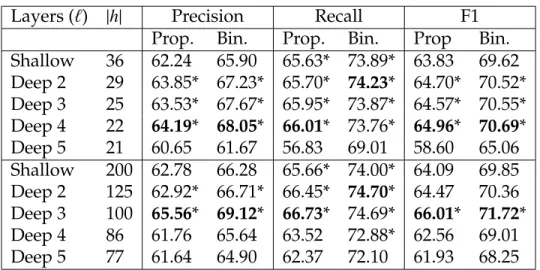
Layers (`) |h| Precision Recall F1
Prop. Bin. Prop. Bin. Prop Bin.
Shallow 36 62.24 65.90 65.63* 73.89* 63.83 69.62 Deep 2 29 63.85* 67.23* 65.70* 74.23* 64.70* 70.52* Deep 3 25 63.53* 67.67* 65.95* 73.87* 64.57* 70.55* Deep 4 22 64.19* 68.05* 66.01* 73.76* 64.96* 70.69* Deep 5 21 60.65 61.67 56.83 69.01 58.60 65.06 Shallow 200 62.78 66.28 65.66* 74.00* 64.09 69.85 Deep 2 125 62.92* 66.71* 66.45* 74.70* 64.47 70.36 Deep 3 100 65.56* 69.12* 66.73* 74.69* 66.01* 71.72* Deep 4 86 61.76 65.64 63.52 72.88* 62.56 69.01 Deep 5 77 61.64 64.90 62.37 72.10 61.93 68.25
Table 3.2: Experimental evaluation of recurrent networks for DSE extrac-tion
Bidirectional vs. Unidirectional. Although our focus is on bidirectional
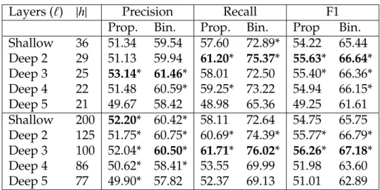
out-Layers (`) |h| Precision Recall F1
Prop. Bin. Prop. Bin. Prop Bin.
Shallow 36 51.34 59.54 57.60 72.89* 54.22 65.44 Deep 2 29 51.13 59.94 61.20* 75.37* 55.63* 66.64* Deep 3 25 53.14* 61.46* 58.01 72.50 55.40* 66.36* Deep 4 22 51.48 60.59* 59.25* 73.22 54.94 66.15* Deep 5 21 49.67 58.42 48.98 65.36 49.25 61.61 Shallow 200 52.20* 60.42* 58.11 72.64 54.75 65.75 Deep 2 125 51.75* 60.75* 60.69* 74.39* 55.77* 66.79* Deep 3 100 52.04* 60.50* 61.71* 76.02* 56.26* 67.18* Deep 4 86 50.62* 58.41* 53.55 69.99 51.98 63.60 Deep 5 77 49.90* 57.82 52.37 69.13 51.01 62.89
Table 3.3: Experimental evaluation of recurrent networks for ESE extrac-tion
Model Precision Recall F1
Prop. Bin. Prop. Bin. Prop Bin.
DSE CRF 74.96* 82.28* 46.98 52.99 57.74 64.45 semiCRF 61.67 69.41 67.22* 73.08* 64.27 71.15* CRF +vec 74.97* 82.43* 49.47 55.67 59.59 66.44 semiCRF +vec 66.00 71.98 60.96 68.13 63.30 69.91 Deep RNT 3 100 65.56 69.12 66.73* 74.69* 66.01* 71.72* ESE CRF 56.08 68.36 42.26 51.84 48.10 58.85 semiCRF 45.64 69.06 58.05 64.15 50.95 66.37* CRF +vec 57.15* 69.84* 44.67 54.38 50.01 61.01 semiCRF +vec 53.76 70.82* 52.72 61.59 53.10 65.73 Deep RNT 3 100 52.04 60.50 61.71* 76.02* 56.26* 67.18*
Table 3.4: Comparison of Deep recurrent networks to state-of-the-art (semi)CRF baselines for DSE and ESE detection
performs a (shallow) unidirectional network for both DSE and ESE recognition. To make the comparison fair, each network has the same number of total pa-rameters: we use 65 hidden units for the unidirectional, and 36 for the bidirec-tional network, respectively. Results are as expected: the bidirecbidirec-tional network obtains higher F1 scores than the unidirectional network — 63.83 vs. 60.35 (pro-portional overlap) and 69.62 vs. 68.31 (binary overlap) for DSEs; 54.22 vs. 51.51
(proportional) and 65.44 vs. 63.65 (binary) for ESEs. All differences are statisti-cally significant at the 0.05 level. Thus, we will not include comparisons to the unidirectional nets in the remaining experiments.
Adding Depth. Next, we quantitatively investigate the effects of adding
depth to recurrent networks. Tables 3.2 and 3.3 show the evaluation of recur-rent networks of various depths and sizes. In both tables, the first group net-works have approximately 24,000 parameters and the second group netnet-works have approximately 200,000 parameters. Since all networks within a group have approximately the same number of parameters, they grow narrower as they get deeper. Within each group, bold shows the best result with an asterisk denoting statistically indistinguishable performance with respect to the best. As noted above, all statistical comparisons use a two-sided paired t-test with a confidence level ofα=.05.
In both DSE and ESE detection and for larger networks (bottom set of re-sults), 3-layer networks provide the best results. For smaller networks (top set of results), 2, 3 and 4-layer networks show equally good performance for cer-tain sizes and metrics and, in general, adding additional layers degrades perfor-mance. This could be related to how we train the architectures as well as to the decrease in width of the networks. In general, we observe a trend of increasing performance as we increase the number of layers, until a certain depth.
Deep recurrent net vs. (semi)CRF. Table 3.4 shows comparison of the best
deep recurrent networks to the previous best results in the literature. In terms of F-measure,DEEPRNT performs best for both DSE and ESE detection,
achiev-ing a new state-of-the-art performance for the more strict proportional overlap measure, which is harder to improve upon than the binary evaluation metric.
SEMICRF, with its very high recall, performs comparably to the DEEP RNT on
the binary metric. Note that recurrent networks do not have access to any fea-tures other than word vectors.
In general, CRFs exhibit high precision but low recall (CRFs have the best precision on both DSE and ESE detection) whileSEMICRFs exhibit a high recall,
low precision performance. Compared to SEMICRF, the DEEP RNTs produce
an even higher recall but sometimes lower precision for ESE detection. This suggests that the methods are complementary, and can potentially be even more powerful when combined in an ensemble method.
Word vectors. Word vectors help CRFs on both precision and recall on both
tasks. However, SEMICRFs become more conservative with word vectors,
pro-ducing higher precision and lower recall on both tasks. This sometimes hurts overall F-measure.
Among the (SEMI)CRF-based methods, SEMICRF obtains the highest F1
score for DSEs and for ESEs using the softer metric; SEMICRF+VEC performs
best for ESEs according to the stricter proportional overlap measure.
Network size. Finally, we observe that even small networks (such as 4-layer
deep recurrent network for DSE and 2-layer deep recurrent network for ESE) outperform conventional CRFs. This suggests that with the help of good word vectors, we can train compact but powerful sequential neural models.
When examining the output, we see some systematic differences between the previously top-performing SEMICRF and the neural models. (See
Fig-ure 3.2.) First, SEMICRF often identifies excessively long subjective phrases as