Design compact and efficient recurrent neural networks for natural language processing tasks

(1)

University of Padua

Department of Mathematics

Master of Science in Data Science

MASTER THESIS

DESIGN COMPACT AND EFFICIENT

RECURRENT NEURAL NETWORKS

FOR NATURAL LANGUAGE

PROCESSING TASKS

Supervisor:

Prof. GABRIELE TOLOMEI

Department of Mathematics

University of Padua (Padua, Italy)

Co-supervisor:

Prof. EKATERINA CHERNYAK

Faculty of Computer Science

National Research University Higher School of Economics

(Moscow, Russia)

Student:

WALTER GENCHI

(2)

(3)

“When you grow up you tend to get told that the world is the way it is and your life is just to live your life inside the world.

Try not to bash into the walls too much. Try to have a nice family life, have fun, save a little money.

That’s a very limited life. Life can be much broader once you discover one simple fact: Everything around you that you call life was made up by people that were no smarter than you.

And you can change it, you can influence it. . . Once you learn that, you’ll never be the same again.”

(4)

(5)

Introduction

The present work takes into account the compactness and efficiency of Recurrent Neural Networks (RNNs) for solving Natural Language Processing (NLP) tasks. RNNs are a class of Artificial Neural Networks (ANNs). Compared to Feed-forward Neural Networks (FNNs), RNN architecture is cyclic, i.e. the connection between nodes form cycles. This subtle difference has actually a huge impact on solving sequence-based problems, e.g. NLP tasks.

In particular, the first advantage of RNNs regards their ability to model long-range time dependencies, which is a very desirable property for natural language data, where word’s meaning is highly dependent on its context. The second advantage of RNNs is that are flexible and accept as input many different data types and representation. This is again the case of natural language data, which can come in different sizes, e.g. words with different lengths, and types, e.g. sequences or trees.

Having said that, it should be noted though that RNNs’ efficacy and execu-tion time are dependent on the size of the network. In particular, these models are often too large in size for deployment on mobile devices with memory and latency constraints. In practice, this means that many simple NLP tasks can be performed only by calling an external cloud server infrastructure, i.e. without the possibility to do the computation offline.

It goes without saying mobile devices are becoming increasignly pervasive in our everyday life, thanks to enabling technologies such asAugmented and Virtual Reality (AR/VR) and Internet of Things (IoT). Moreover, an always increasing number of deep learning applications on such mobile devices are required to run inreal-time, e.g. pedestrian detection in an autonomous vehicle.

For these reasons, industry practitioners and academic researchers are asked to design neural network models which can be stored on device (space-efficiency) and produce fast predictions (time-efficiency) with very little performance loss (effectiveness). This has started a new research field named model compression by Bucilua et al. (2006), which has proposed in the recent years solutions coming from many disciplines, including but not limited to machine learning,

(8)

optimiza-Contents

tion, computer architecture, data compression, and hardware design.

The first objective of this work is to understand and categorize the state-of-the-art neural network compression techniques. Most of these compression methods have been applied Deep Neural Networks (DNNs) and Convolutional Neural Net-works (CNNs), while only a small attention has been given to compressing RNN architectures when solving NLP tasks.

Therefore, the second objective is to apply two different compression methods on a multi-layer RNN architecture, which has been trained to perform a simple NLP task, i.e. Part-of-Speech Tagging (PoS Tagging). After evaluating a naive application of these compression methods, we will propose and evaluate more tailored compression methods, based on the distribution of redundancy in the LSTM architecture.

The present work is divided in two wide content areas. The first two chapters of the thesis are a gentle introduction to NLP and Neural Networks, while the last two chapters are entirely devoted to RNNs.

Chapter 1 gives an overview on the characteristics and challenges of natural language data when solving NLP tasks. Moreover, an example of the typical pipeline of feature design and feature embedding in a concrete NLP task will be provided. A final discussion about the reasons of the success of Deep Learning in NLP will close the chapter.

Chapter 2 provides an introduction to Supervised Learning and Feedforward architecture, which will be useful later when considering PoS Tagging as a clas-sification problem and RNN architectures as a specialized neural network archi-tecture. After discussing the advantages of Multi Layer Perceptron (MLP) over Linear Models in terms of representational power, the last part of this chapter is devoted to optimization and regularization strategies, gradient computations and best practices when training a neural network.

Chapter 3 presents the RNN high-level abstraction, graphical representations (recursive and unrolled) and architectural variations (bidirectional RNNs and deep RNNs). Finally, three concrete recurrent architectures (Simple RNN, LSTM and GRU) will be described in details.

Chapter 4 firstly conducts a literature review on existing neural network com-pression methods and metrics and eventually identifies four general approaches, i.e. Matrix Factorization, Parameter Pruning, Parameter Sharing and Quanti-zation. After that, the focus goes on an extensive description of the Universal Dependencies (UD) dataset, which has been used for training and evaluating a multi-layer LSTM model on a PoS Tagging task. The final part of this chapter

(9)

Contents

presents the conclusions and take-home messages, based on the results obtained from the different compression strategies implemented.

(10)

(11)

Mathematical Notation

For the sake of simplicity, we keep the same mathematical notation from Goldberg (2017):

• Matrices and vectors are represented with capital and lower case bold letters respectively, e.g. W for matrices and xfor vectors.

• Vectors are assumed to be row vectors, i.e. the d-dimensional vector x has

size 1×d.

• The i-th element of vector xis indicated as x[i].

• The element in the i-th row and j-th column of matrix W is indicated as wij.

• The j-th element of a sequence w1:n=w1, w2, . . . , wn is indicated as wj. • Vector concatenation of vectors x1 and x2 is written as[x1;x2].

(12)

(13)

1 What is Natural Language

Processing?

Natural language processing (NLP) is a subfield of computer science, information engineering, and artificial intelligence concerned with the interactions between computers and human (natural) languages, in particular how to program com-puters to process and analyze large amounts of natural language data.

The first consideration regards the definition of NLP. Jurafsky and Martin (2008) claim that NLP cannot be defined as an independent scientific field, but it is rather an “interdisciplinary field with many names corresponding to its many facets, names like speech and language processing, human language tech-nology, natural language processing, computational linguistics, and speech recog-nition and synthesis”. In other words, the current NLP methods and algorithms are nothing but the result of a 50-year research involving experts from linguis-tics, computer science, electrical engineering and psychology. Given the strong linguistic component in NLP, in section 1.1 we will present the main linguistic challenges in common NLP tasks. These have been combined in more complex tasks and finally deployed by the industry in successful tools that are already part of our everyday life.

Secondly, NLP has the goal to provide computers with the “knowledge of lan-guage”(Jurafsky and Martin, 2008). The main obstacle is the nature of the input, i.e. natural language data, which is by definition ambiguous and variable. In section 1.2, we will examine in details the characteristics and challenges of pro-cessing natural language data. Moreover, we will introduce two design approaches when selecting not only the intrinsic features (single word), but also the extrinsic features (word in context). Note that such linguistic features have to be first en-coded into an embedding vector, which can be then given as input to a machine learning model (in our case a RNN). This process is called feature embedding and it is described in details by using a concrete example on the Part-of-Speech Tagging task.

(14)

1 What is Natural Language Processing?

solving NLP task. Such models are indeed able to spot patterns and regularities in the training data and, eventually, generalize this ability to a set of previously unseen data. In section 1.3, we will see not only the reasons behind the success of deep learning in the NLP domain, but also the advantages of specific deep learning models, i.e. RNNs, for some specific NLP tasks. This will give the key ingredients for the next chapter, which will be focused on RNN models.

The reference literature for this chapter is Jurafsky and Martin (2008) regarding the linguistic challenges in NLP and Goldberg (2017) regarding the mathematical notation and specific terminology for NLP concepts, which will be also used in the following chapters.

1.1 NLP in everyday life

Nowadays it is not rare to start a conversation with some virtual assistants directly on our smartphones: “Hey Siri, what is the weather like today in Moscow?” could be one of the first questions in the morning. In order to be

able to interact with the user, these complex systems perform several NLP tasks and have to overcome many linguistic challenges.

The first task these systems perform is called Speech Recognition, i.e. they should be able to traslate spoken language into a correct sequence of words. In order to do that, they should have knowledge about how words’s sounds are pronounced in terms of sequences of sounds. This type of knowledge is called phonetics in linguistics.

Once the answer has been elaborated by the system, the task of Speech Syn-thesis consists in organizing the sounds for the answer, i.e. artificially traslate text to human speech. This ability is studied byphonology in linguistics.

Once the conversation has gone further, the user may ask “What are the main events in the weekend?”. This type of question assumes that the

dialogue system keeps track of previous parts of the discourse, i.e. we are inter-ested in the events in the city of Moscow. In NLP this task is calledCoreference Resolution.

Another very likely possibility is that the user’s question may be ambiguous, i.e. there are many meanings which can be attributed to the same word. “Where can I eat a pizza with friends?” has a very different meaning from “Where can I eat a pizza with salami?”, even tough they differ in only one word.

Here lies the ambiguity of human language, which is solved by Disambiguation tasks. One example of lexical disambiguation in NLP is Part-of-Speech (PoS)

(15)

1.2 Data Preprocessing in NLP

Tagging, which tags each word with a particular part of speech (e.g. noun, verb, adjective etc.). 1 We will see more about PoS Tagging task in section 1.2.

These are only some examples of the numerous NLP tasks currently studied by research and industry practitioners. A common pattern in NLP is that simple (but not trivial) tasks, e.g. PoS Tagging, are used to solve more complex tasks, e.g. Coreference Resolution. In the next sections we will explore the whole pipeline of natural language data preprocessing, which is a preliminary step in all NLP tasks.

1.2 Data Preprocessing in NLP

According to Goldberg (2017), human (natural) language data is very challenging from a computational point of view, since it is highly discrete, compositional and sparse.

The property of discreetness regards the nature of input (symbols), which are not necessary related to the meaning of the word itself. As an example, consider image data: there exist some filters (i.e. mathematical operators) to convert an image from color to greyscale. The samecontinuous relationship cannot be found between words red and grey.

Having said that, the meaning of individual words and the relationship between different words can be found by looking at the composition (sequence) of words in a sentence, in a paragraph or even in the whole document. This arises the issue of long-range dependencies between words in a document, which led to the success of RNNs for some specific tasks, e.g. Language Modeling (see section 1.3). All in all, human language is sparse: it is highly variable, i.e. there are poten-tially infinite ways to combine words. Moreover, it is hard to generalize, which is the final goal of all machine learning models.

In the next section we will see firstly the design approaches to select the relevant features according to the NLP task. Moreover, it will be presented an overview of the mathematical methods used to convert linguistic features into an embedding vectorx.

Feature Design for NLP Problems

The process of feature selection (also called feature engineering) is one the most crucial and, at the same time, delicate in any machine learning task. The NLP

1_{Hereafter we assume that the tokenization task, e.g. separating words from punctuation, has}

(16)

community has tried to design relevant features for textual data, by looking at the properties of natural language data.

Disclaimer Before starting the discussion on feature design in NLP, here is an important disclaimer to the reader.

Textual data can come in different forms and sizes: the typical hierarchical structure is document, paragraph, sentence, word and finally character. A typical option is to consider word-level models, i.e. the input is a sequence of n words

(w1, . . . , wn). In section 3.4, we will see an alternative character-level model for

RNNs, i.e. the input is a sequence of N characters (c1, . . . , cN).

Intrinsic vs. Extrinsic Features The main idea for feature selection in NLP is to divide the source of information into two categories: intrinsic features (word-dependent) andextrinsic features (context-dependent).

Intrinsic features analyse each word individually, i.e. they do not carry any information about neighbor words. In PoS Tagging task, for example, some useful intrinsic features are prefixes, suffixes and orthographic shape. For example, if an English word’s suffix ising, then it is very likely a present-continuous verb.

However, as we explained in section 1.1, human natural language is by definition ambiguous and variable. This means that typically the meaning of a word is not exclusively word-dependent, but its interpretation is also context-dependent. Having said that, extrinsic features typically focus on the close neighbors of wj,

e.g. a window ofk words to each side, centered in positionj.

This window-approach is useful to model sequence data because it takes into account the relative position of the words. However, in NLP community is it well-known that “sentences in natural language have structures beyond the linear order of their words. The structure follows an intricate set of rules that are not directly observable to us”(Goldberg, 2017).

In particular, fixed-sized windows are not able to model long-range dependen-cies, e.g. a word at the beginning of a sentence is linked with a word at the end of the sentence. This behavior is actually very common in human language. Therefore, some alternative models have been proposed: for example, Bidirec-tional Recurrent Neural Networks (biRNNs) presented in section 3.4 provide a window with flexible and adaptive size.

Directly Observable vs. Inferred Linguistic Properties Another convenient feature categorization in NLP is betweendirectly observableandinferred linguistic properties.

(17)

The first set of properties is derived directly from the input, by following some predefined algorithmic procedures, which typically involve counting operations, e.g. word frequency in the bag-of-words (BOW) approach (see section 1.2), and boolean operations, e.g. word position in a sentence. Other notable examples are lemmatization and stemming, which are both governed by linguistically-predefined rules and thus may not produce an appropriate output in all contexts. The second set of properties is based on well-known concepts in linguistics, e.g. word classes (e.g. PoS tags), morphology,syntax and semantics. In practice, the results obtained from some of thesespecialized NLP tasks, e.g. PoS tags, are first combined and then used as predictors for solving more sophisticated classification tasks.

Human vs. Automatic Feature Design The process for getting such human -designed features can be subject to error and is time-consuming, since it requires specialized expertise in the linguistics field.

This approach to feature design is actually in contrast with the dominant trend nowadays in NLP. In fact, deep learning practitioners claim that neural network are able to automatically represent these linguistic concepts in the intermediate layers of the network. This aspect will be further discussed in section 1.3.

Feature Embedding: from Linguistic Features to Embedding

Vectors

In the previous section we have discussed the popular approaches when deciding which linguistic features actually carry useful information for solving our specific NLP task.

The next step is to represent each of the k liguistic features fi (sparse

sequence of discrete symbols over a vocabulary V) into an embedding vector

v(fi)2 (dense and with fixed size d).

The resulting embedding vectors v(fi) can be later combined (either by

con-catenation, summation or mix of both) into an input vectorx using a feature function φ(·). Now x is a well-defined mathematical object and can be later

given as input to other machine learning models, e.g. neural networks.

2_{Note that}_v₍_·₎_{is a function operator. This is the reason why we will not use bold notation}

(18)

One-hot Encodings

The first and most elementary way to econde textual data is the Bag-of-words (BOW) representation, which is widely used for document classification.

The main idea of BOW is to characterize a document by the words contained in it, i.e. think aboutindicator functions (which words are present in the document). The BOW representation does not take into account the order of the words.

For example, if we take the document s1 =“My name is John Smith” over a vocabulary V of 10,000 items, s1 will be represented by a very sparse 10,000-dimensional vector in which 5 elements have non-zero entries (ins1 all words are different3_).

Following this representation, if word name has for example position 7332 in V, then it is mapped into a 10,000-dimensional one-hot vector, where the only non-zero entry is in position 7332.

One of the weaknesses with such encoding scheme is that features are treated as fully indipendent from one another, e.g. the dissimilarity between words_orange andlemonis the same as the one between orange andname. Moreover, from

a computational point of view,high-dimensional andsparse vectors are not easily handled by neural networks.

Dense Econdings

A more convenient representation of any linguistic feature fi is the embedding

vectorv(fi), which isdense (not sparse) and has fixed size d |V|.

It can be easily shown that this representation is actually related to the one-hot econding seen before. Letfi be the one-hot encoding of the linguistic featurefi,

i.e. a |V|-dimensional vector. If we stack (vertically) the d-dimensional

embed-ding vectors v(fi), we obtain the embedding matrix E with dimension |V| ×d.

Now we can establish the equalityv(fi) =fiE, i.e. we select the i-th row of E.

The main benefit of such dense representation is the generalization power. Take as an example the Named-entity Recognition (NER) task. Our goal is to correctly identify and classify the named entities, e.g. London, Rome, James Cameron, Federico Fellini, etc. It may happen that in our training set we

have observed many times the words Rome and Federico Fellini, but only

few timesLondon.

A good embedding vector will be able to tell us that _London is a city, so it is like Rome, and thatJames Cameron is a film director, so it is like Federico

3_{Note that}

My and my are considered as different words if capitalization has been removed

or if the capitalization status of wordwj has been included in the linguistic features.

(19)

Fellini. Therefore, our model will still be able to generalize, i.e. London will

be correctly labeled as a city in the sentence “James Cameron has made a great movie in London”.

Learn Embedding Vectors

In practice, we do notlearn embedding vectors v(·) for every NLP task. Instead, we use pre-trained embeddings, which have been already trained on a huge quan-tities of unannotated text.

The motivation behind such an approach is thatwords are similar if they appear in similar context, i.e. according to the context, similar words will have similar embedding vectors. This assumption is called thedistributional hypothesis in the NLP community.

Having said that, it should be noted that for some NLP tasks the pre-trained embeddings are not left fixed during the network training process, but instead they are further-tuned.

The most popular word embedding algorithms available are Word2Vec and GloVe.

Example: Part-of-Speech Tagging

Here is an example of data preprocessing required for the Part-of-Speech Tagging task, describing the whole pipeline from the feature design stage to the feature embedding stage. The example is taken from Goldberg (2017).

Just to refresh memory, PoS Tagging is a lexical Disambiguation task in NLP. The goal is to tag each word with a particular part of speech (e.g. noun, verb, adjective etc.). Following what has been done by Goldberg (2017), the tagset comes from theUniversal Treebank Project and contains 17 tags.

Feature Design

We assume that when the classifier has to predict the tag for word wj, it has

access only to a small neighbor, e.g. wj−2,wj−1, wj+1, wj+2, and not to the whole

sentence w1, . . . , wn.

For example, immagine we want to perform PoS Tagging task on the sentence “Tonight I will have a pizza with my friends”.

For j = 1, . . . , n, we take into account the following _{intrinsic features}

for word wj:

(20)

• 2 and 3-letter prefix of wj, i.e. pref(wj,2)and pref(wj,3) respectively

• 2 and 3-letter suffixof wj, i.e. suf(wj,2)and suf(wj,3) respectively

• vector of boolean variables cj for wj (yes=1, no=0): word-is-capitalized,

word-contains-hyphen and word-contains-digit

We take into account the following extrinsic features for word wj:

• For t=−2,−1,+1,+2 (window of size 2) – the neighbor word wj+t

– 2 and 3-letterprefixof neighbourwj+t, i.e. pref(wj+t,2)andpref(wj+t,3)

respectively

– 2 and 3-lettersuffixof neighbourwj+t, i.e. suf(wj+t,2)andsuf(wj+t,3) respectively

– vector ofbooleanvariablescj+tfor neighbourwj+t: word-is-capitalized,

word-contains-hyphen and word-contains-digit • For t=−2,−1 (previous 2 words)

– Predicted PoS for word wj+t, i.e. pˆj+t

Feature Embedding

The next step is to encode the linguistic features for word wj into a vector vj,

which summarizes the information coming from wordwj.

We use four different embedding functions with different dimensions4_: _v

w(·)∈

Rdw for_words,_v

p(·)∈Rdp for prefixes,vs(·)∈Rds for suffixes and vt(·)∈Rdt for

tags.

Overall, vj can be written as a concatenation

vj =   cj |{z} BOOL ;vw(wj) | {z } W ORD ;vs(suf(wj,2) | {z } 2−SU F F ;vs(suf(wj,3) | {z } 3−SU F F ;vp(pref(wj,2) | {z } 2−P REF ;vp(pref(wj,3) | {z } 3−P REF  

and hasdimension

vj ∈R BOOL z}|{ 3 + W ORD z}|{ dw + SU F F z}|{ 2ds+ P REF z}|{ 2dp _.

4_{This is an example where}_d_{can change for different feature types}

(21)

For example, the information for the word _pizza can be summarized in the vector v_pizza =  (0,0,0) | {z } BOOL ;vw(pizza) | {z } W ORD ;vs(za) | {z } 2−SU F F ;vs(zza) | {z } 3−SU F F ; vp(pi) | {z } 2−P REF ;vp(piz) | {z } 3−P REF  

Finally, the input vector x will be the result of the concatenation of the embedding of extrinsic features, intrinsic features and previous tags

x=φ(s, j) =



vj−2;vj−1

| {z }

EXT RIN SIC

; vj

|{z}

IN T RIN SIC

;vj+1;vj+2

| {z }

EXT RIN SIC

;vt(ˆpj−2);vt(ˆpj−1) | {z } P REV IOU S T AG   and dimension x∈_R W IN DOW z}|{ 5 1EM BEDDIN G z }| { (3 +dw+ 2ds+ 2dp)+ T AG z}|{ 2dt _.

For example, in the sentence “Tonight I will have a pizza with my friends”, the input vector x for the wordpizza is

x=φ(s,_pizza) =



 v_have;v_a | {z }

EXT RIN SIC

; v_pizza

| {z }

IN T RIN SIC

; v_with;v_my

| {z }

EXT RIN SIC

;vt(ˆphave);vt(ˆpa) | {z } P REV IOU S T AG  . Discussion

The first consideration when using such an approach regards thecomputation of the vectors vj.

Since we use the same embedding functionvw(·)for every wordwj, we actually

have to learn only one embedding table, i.e. matrixE. Therefore, the

computa-tionvw(wj)is quite cheap, since it is performedonly once and the result is reused

for different positions j. Moreover, this approach stores the information about

the relative position of the words in the sentence, i.e. some information is shared between different input vectors x and therefore their statistical strength in the

model is increased.

The second consideration is aboutword-capitalization. In the previous example, the embedding vectors for the wordsTonightand tonightare different. Since

we are already take into account the capitalization of word wj in the boolean

vector cj, this information will result to be redundant in the input vector x. If

we decide to keep the vector cj, then it is better to lower-case all words in our

(22)

Another source of redundancy may be the 2 and 3-letter prefix and suffix feature. In order to overcome this problem, one possibility is consider character-level models, instead of word-character-level models. As we will see in section 3.4 with character-level RNNs, this approach augments data granularity and is suitable for spotting specific patterns and regularities in the words.

Finally, we should always take into account that some words, e.g. pizza,

may not be present in our vocabulary V. Such unkown words are called out-of-vocabulary (OOV) items and they are mapped to the special symbol _Unk.

1.3 The Advent of Deep Learning in NLP

It was at the end of the 20th century that NLP experienced the so-calledstatistical revolution(Johnson, 2009). According to Jurafsky and Martin (2008), three main factors determined such a big change in the field:

1. Popularity of probabilistic and data-driven models over knowledge-based methods.

2. Steady increase ofcomputational power allowed the deployment of commer-cial NLP tools.

3. The rise of the Web increased data availablity and imposed the need to develop language-based information retrieval.

Since the beginning of the 21st century, Deep Learning has dramatically changed again NLP. According to Goldberg (2017), two main factors have determined the success of deep learning over other machine learning models:

1. The use of the embedding layer to map textual data (discrete and sparse) to a feature-vector (continuous and low-dimensional).

2. The flexibility of RNNs to model sequence data and consequently the aban-don of markov assumption.

Embedding Layer and Representational Learning

The concept of embedding layer in NLP is actually an instance of a much more general concept in machine learning: representational learning (Goodfellow et al., 2016). In general, this concept means that a machine learning algorithm learns not only to correctly predict the target output, but learns also how to correctly represent the data.

(23)

1.3 The Advent of Deep Learning in NLP

In the deep learning domain, such representation is learned by successive ap-proximations (from the early layers to the last layers) of the input data. In the last years, this feature has become very popular also in other domains and ac-tually led to the development of specialized architectures for different tasks, e.g. Convolutional Neural Networks (CNNs) for Image Recognition tasks and Recurrent Neural Networks (RNNs) for NLP tasks.

Feedforward Neural Networks

The concept of representational learning can be easily understood when consid-ering the first and simplest class of artificial neural network architectures, i.e. Feedforward Neural Networks.

As already mentioned, specialized recurrent architectures are actually a modi-fication of the feedforward architecture. Therefore, the key intuitions behind the concept of representational learning can be first derived from feedfoward archi-tecture and then generalized to the recurrent archiarchi-tecture. Having said that, the goal of Chapter 2 is to introduce the reader to the key concept of representational learning, by presenting the Multiple-layer Perceptrons (MLPs) abstraction and its advantages compared to the traditional linear models, e.g. Logistic Regression. The first advantage of feedforward neural networks over linear models regards therepresentation power. In particular, it has been shown that MLP1(MLP with a single hidden layer) is a universal approximator, i.e. any input can be mapped from any finite dimensional discrete space to another.

The second advantage is that MLP architecture implements a trainable non-linear mapping function, which is a particularly useful feature when the nonlinear-separability condition does not hold in the training data. This is definitely the case in NLP, where the input is discrete and highly sparse.

Reccurent Neural Networks

So far we have seen that MLPs are excellent alternatives to the standard linear models for classification tasks, given their ability to learn in principle any repre-sentations of the data, regardless the nonlinearity and complexity of the input. However, MLPs are general-purpose classification architectures and thus they are not tailored for specific NLP tasks, e.g. Language Modeling.

For this reason, in Chapter 3 we will discuss another class of artificial neural networks, i.e. RNN architecture. In particular, we will present the RNN high-level abstraction, graphical representations (recursive and unrolled) and architectural

(24)

variations (biRNNs and deep RNNs). Finally, three concrete recurrent architec-tures (Simple RNN, LSTM andGRU) will be presented in details in sections 3.2 and 3.3.

Compact Recurrent Neural Networks

One typical problem of deep neural networks is that their efficacy and execution time are dependent on the size of the network. In particular, these models are often too large in size for deployment on mobile devices with memory and latency constraints.

In our NLP framework, this means that many simple NLP tasks can be per-formed only by calling an external cloud server infrastructure, i.e. without the possibility to do the computation offline.

The first objective of Chapter 4 is to understand and categorize the state-of-the-art compression techniques already available. The goal is firstly to understand the rationale behind each of these technique and secondly to go through the mathematical details and implementations of the methods. In the mean time, the second objective is to apply these compression techniques on some simple NLP tasks (Language Modeling, Part-of-speech Tagging, Named Entity Recognition, Chunking), in order to compare the compact model with the full model and eventually to spot the distribution ofredundancy in the RNN architecture.

RNNs and Markov Assumption

One strong prerequisite for any NLP model is the ability to take into account the dependency structure in sequencial data, e.g. a sentence s made of w1, . . . , wn

words.

In the last decades, the traditional approach in NLP was to restrict the frame-work and simply to condition the wordwt+1 on a fixed-size (e.g. with sizek) past sequence wt−k, . . . , wt. This assumption is called k-th order Markov assumption in probability theory and generally refers to the memoryless property of stochastic processes.

The main issue with the Markov assumption is the nature of the input. As we have already discussed in section 1.2, textual data is highly ambiguous and variable. Ambiguity imposes to take into account the context of word wt+1 in a sentence, e.g. the lastkwords in the sequence. At first sight, Markov assumption

fits the NLP framework. However, variability of textual data injects randomness in the input, which consequently makes it difficult to a-priori set a proper value

(25)

1.3 The Advent of Deep Learning in NLP

for k.

RNNs solve this issue by allowing flexible and trainable windows of arbitrary size. This feature represented an incredible improvement in many important NLP tasks, e.g. Language Modeling.

Having said that, simple RNNs architectures have still some issues. In a sen-tence or in a longer text, the context and consequently the meaning of a word does not necessarily depend only on the past words. For example, in Handwriting Recognition task, where the goal is to convert handwritten input (noisy) to letter codes (bits), the prediction on the target letter can be improved by taking into account the letters coming after it.

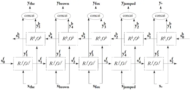
Bidirectional Recurrent Neural Networks (biRNN) modify the training step of traditional RNNs, by presenting two version of the input sequence (original and reversed) to two separate RNNs. The final prediction is based on both RNNs outputs. The details are discussed in section 3.4.

Research Areas

Two promising research areas in the deep learning and NLP domains are Multi-task Learning (MTL) and Semi-supervised Learning.

MTL has the goal to improve the performance in a given NLP task, by com-bining the information from other NLP tasks. This approach is motivated by the intimate relationship between NLP tasks, as already seen in section 1.1.

Semi-supervised Learning wants to improve the accuracy on one task, by ex-ploting data which have been annotated or unannotated for other tasks. Data annotation is unfortunately a very delicate, costly and time-consuming process.

(26)

(27)

2 Feedforward Neural Networks

Nowadays, it is extremely popular to see feedforward neural networks in many machine learning applications both at academic and industrial scale. As already mentioned in the previous chapter, this increase in popularity led to the devel-opment of specialized architectures for different tasks, e.g. Convolutional Neural Networks (CNNs) for Image Recognition tasks and Recurrent Neural Networks (RNNs) for NLP tasks.

The aim of this Chapter is to take a conceptual step back, before going into the details of RNNs and their applications to NLP tasks.

In section 2.1 we will review the key concepts behind supervised learning algo-rithms, which are one of the most used in several machine learning applications. The theorethical concepts of hypothesis class and inductive bias will be presented together with a simple example of parametric supervised learning algorithms, i.e. Linear Models. This will introduce the limits of linear models and so the need to perform nonlinear transformation on the input, when dealing with linearly non separable data. Three different startegies will be presented, which will eventu-aly lead to the choice of Multi Layer Perceptrons (MLPs) due to their univerisal representation power.

In section 2.2, after describing the differences between recurrent and feedfor-ward architectures, we will mathematically define Artificial Neuron, Single Layer and Multi Layer architectures. Moreover, it will be introduced the concept of activation function and representation power in neural networks.

The last section of this Chapter is devoted to the design choices which have to be made when training a neural network. The largest difference between lin-ear models and neural networks is that the neural network nonlinlin-earity causes most interesting loss functions to become non-convex. Therefore, the optimiza-tion process is iterative and gradient-based and usually requires computing the gradients of complicated functions. The popular algorithm is Backpropagation and its implementation is usually based on the Computation Graph Abstraction. This algorithm will be extended to RNNs, where it will be called Backpropagation through time.

(28)

2 Feedforward Neural Networks

The neural network’s notation and figures of this chapter are taken from Gold-berg (2017). The exposition of the main ideas from machine learning and neural network’s training are inspired by the work of Goodfellow et al. (2016).

2.1 Supervised Learning

Consider a functional dependency that maps points from an input spaceX ∈_Rdin to an output space Y ∈_Rdout.

In a typical supervised learning task we are given a training set T of n

input-target pairs(xi,yi), i.e.

T ={(xi,yi) :xi ∈X,yi ∈Y and i= 1, . . . , n}.

The goal of supervised learning is to define a mappingf and produce a prediction ˆ

y=f(x), which correctly predicts the true output y.

When dealing withclassification problems, the input space Xis divided intoK

subsetsX1, . . . , XK ∈X such that Xi∩Xj =∅ for all i, j = 1, . . . , K and i6=j.

Now the task is to assign a given input vectorx to the subset it belongs to.

The basic form of any classification task is thebinary classification, where there are two setsX1, X2 ∈X such thatX1∩X2 =∅and we want to determine whether the input vector x belongs toX1 or X2. In this case, the training set is formaly defined as

Tbinary ={(xi, yi) :xi ∈X, yi ∈ {−1,+1} and i= 1, . . . , n}

with the two subsets X1 and X2 labelled by +1 and −1, respectively.

Linear Model and Nonlinear Input

It goes without saying that the set of all possible functions f is extremely large.

What is tipically done in practice is to restrict our search only to some families of functionsf, calledhypothesis classes, where all the elements in this family share some propreties, e.g. parametric supervised learning algorithms.

This is the case of Linear Models, which come in the form

f(x; Θ) =xW +b

x∈_Rdin_,_W _∈

Rdin×dout,b∈Rdout Θ = W,b

(29)

2.1 Supervised Learning

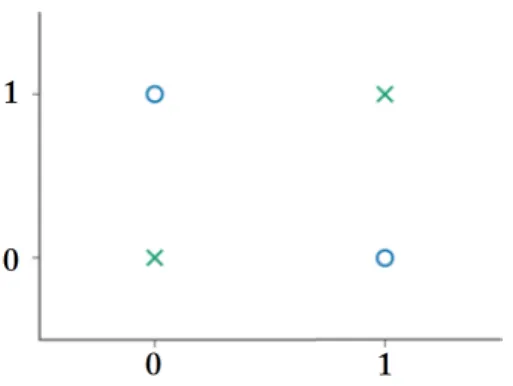
Figure 2.1: XOR function: green crosses belong to class -1, while blue circles belong to class +1.

and we assume that outputycan be represented as a linear combination of inputs

x.

For example, in binary classification the linear model assumes that there exists a hyperplane which can perfectly separate the two set of pointsX1andX2, i.e. the linear separability condition holds. In machine learning, this type of assumptions on the model are called inductive bias.

A simple example where the linear assumption is not verified is the XOR prob-lem. The XOR function is defined as

XOR(0,0) = −1 XOR(1,0) = +1 XOR(0,1) = +1 XOR(1,1) = −1 and is graphically represented in Figure 2.1.

In order to make linear models able to represent nonlinear functions of x, one

could apply the linear model to a trasformed inputφ(x), whereφ(·)is a nonlinear function.

The question now is how to choose a suitable φ:

1. Use a very generic φ. This is the solution generally proposed by kernel methods, where xis projected into a high-dimensional (even infinite) space φ(x), where the linear model can fit well the training data. The main issue with such an approach is the poor generalization ability of the model. 2. Use a manually-designed φ. This approach belongs to the past and is

(30)

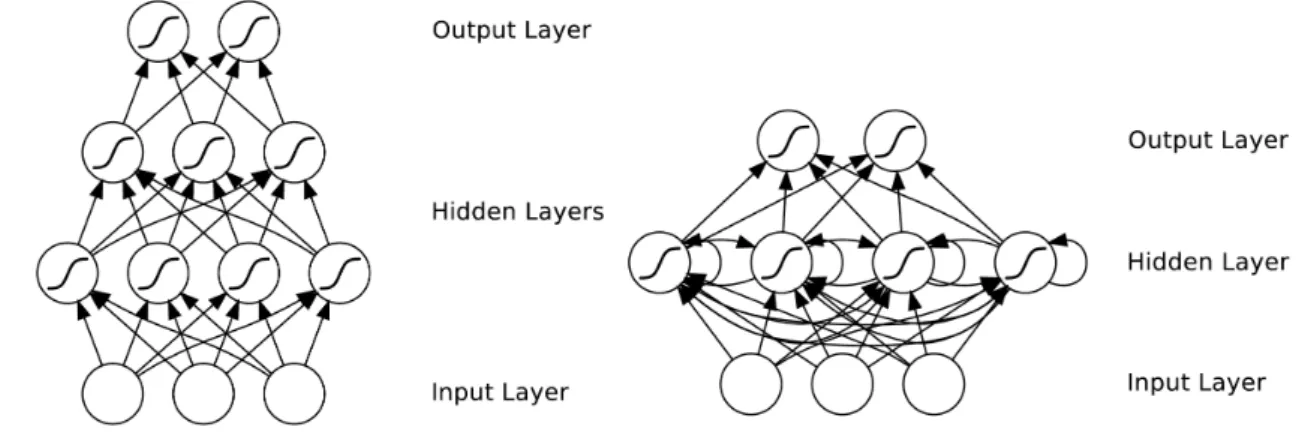
Figure 2.2: Feedforward (left) and Recurrent (right) architecture.

is highly dependent on the dataset and does not allow transfer learning between domains.

3. Use a trainable φ. This is the case of feedforward neural networks and

it represents the core of representational learning. In this case the final prediction yˆ is based on two steps: the neural network first learns φ from

a broad class of functions and then it maps φ(x) to the desired output

ˆ

y. As we saw in the previous chapter, representational learning means

that a machine learning algorithm learns not only how to correctly predict the target output y, but it learns also how to correctly represent the data

through φ(x).

In the next sections we will see in detail the Multilayer Perceptron architecture and some general ideas about neural network training.

2.2 Feedforward Architecture

Artificial Neural Networks (ANNs) have appeared in the past in different archi-tectures and related propreties, according to the task they were designed to solve. The main distinction in ANNs regards the presence or not of cycles in their graph. ANNs with cycles (see Figure 2.2 on the right) are called Recurrent Neural Networks (RNNs) and are dealt with in Chapter 3. ANNs without cycles (see Figure 2.2 on the left) are referred to as feedforward neural networks (FNNs) and are explored in this section.

(31)

2.2 Feedforward Architecture

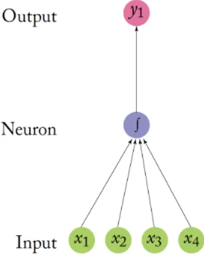
Figure 2.3: Single Artificial Neuron with 4 (scalar) inputsx1, x2, x3, x4.

Artificial Neuron

Using a metaphor from the biology and neuroscience field, an artificialneuron is nothing but the node of an ANN graph. In other words, a neuron represents the elementary computational unit of a neural network.

For example, the neuron in Figure 2.3 takes 4 scalars x1, x2, x3, x4 as input with associated weights w1, w2, w3, w4 (not shown in the picture, but graphically corresponding to the 4 arrows from inputs to the neuron).

The operations performed by the neurons are the following: • Multiply each input xi by its weight wi

• Sum them up, i.e. P4

i=1

xiwi

• Apply a nonlinear function g (called activation function and shown as R in

figure 2.3) to the previous result, i.e. g( 4

P

i=1

xiwi)

• Pass the priovious result to the output, i.e. y1 =g( 4

P

i=1

xiwi)

In ANNs neurons are connected to each other, forming the so-called neural net-work.

Single Layer Perceptron

As a linear classifier, the simplest feedforward neural network is the single layer perceptron, which can be written in mathematical terms as

(32)

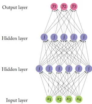
Figure 2.4: Multi Layer Perceptron with two hidden layers (MLP2).

NNSingle Layer Perceptron(x) = xW +b

x∈_Rdin_,_W _∈

Rdin×dout,b∈Rdout Θ = W,b

and in fact coincides with the linear model introduced in Section 2.1 and therefore has the same limitations when dealing with nonlinear input.

Multi Layer Perceptron

The limits of linear functions can be overcome by adding one or more non-linear hidden layers in the network. The result is the Multi Layer Perceptron (MLP) architecture.

An example of feed-forward neural network with two hidden layers (MLP2) is represented in Figure 2.4.

More generally, a MLP2 can be mathemathically written as:

(33)

2.2 Feedforward Architecture NNMLP2(x) = y h1 =g1(xW1+b1) h2 =g2(h1W2+b2) y =h2W3 x∈_Rdin_,_y_∈ Rdout W1 ∈_Rdin×d1_,_b1 _∈ Rd1,W2 ∈Rd1×d2,b2 ∈Rd2,W3 ∈Rd2×dout Θ =W1,W2,W3,b1,b2

Compared to the example of Figure 2.3, the network in MLP2 is now described in terms of vectors and matrices:

• Input xand outputy are vectors with dimension din and dout respectively.

• Weights and bias terms of layer l1 _{are stored in matrices}_Wl _{and vectors}_bl

respectively. • Weight wl

ij represents the connection from thei-th neuron in layer l to the j-th neuron in layer l+ 1.

• The activation function gl is applied element-wise.

In a multilayer perceptron architecture, neurons are arranged in layers, with connections feeding forward from one layer to the next. The length of this chain of connections gives the model’sdepth, from which comes the word deep learning. Input patterns are presented to the input layer, then propagated through the hidden layers to the output layer. When layer hl in the network is the result

of a linear transformation of the input, then it is called fully-connected layer. Other types of layers are for exampleconvolutional andpooling layers, which are particularly useful in immage recognition tasks.

The next parts of this section are devoted to some further discussion on the MLP architecture.

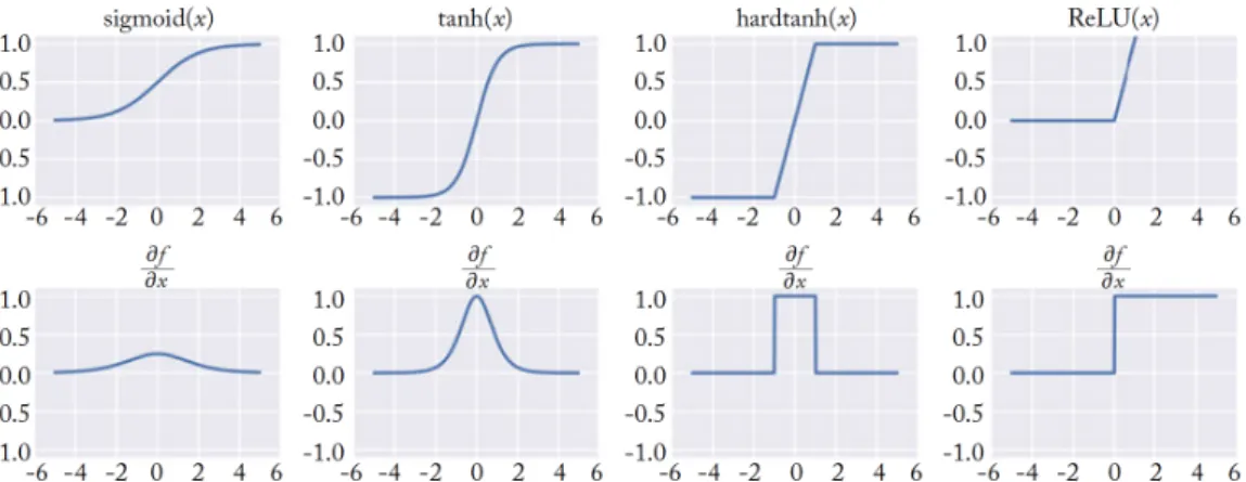
Activation Functions

In the MLP architecture, the activation function is applied to each neuron’s value before passing it to the output. Figure 2.5 shows some common choices of activation functions g and their derivativesg0.

(34)

Figure 2.5: Four common Activation Functions (top) and their Derivatives (bot-tom).

The most popular activation functions are the hyperbolic tangent and the sig-moid functions, which are differentiable and thus allow the network to be trained with gradient descent, as we will see in Section 2.3.

Having said that, in general the choice of g is really task-dependent. For

example, for binary classication tasks the standard configuration in the output layer is a single unit with a sigmoid activation function.

What these activation functions have in common is their nonlinearity. This is the reason why Multi Layer Perceptron is more powerful than Single Layer Perceptron, since it can succesfully deal with non-linear classication boundaries and model non-linear equations. Note that any MLP with linear hidden layers (i.e. gl _{is linear for all} _l_{) is exactly equivalent to the Single Layer Perceptron,}

since any combination of linear operators is itself a linear operator. Here lies the advantage of using nonlinear activation functions: the neural network can first learn how to correctly represent the inputx at successive hidden layers and then

predict the output y, based on this new representation of x.

Representation Power

Going back to the beginning of this chapter, the goal of supervised learning is to define a mapping yˆ and produce a predictionyˆ=f(x), which correctly predicts the true outputy.

A MLP can actually provide a wide range of different functionsf to map from

input xto the desired output y. In particular, it has been proven that an MLP

with a single hidden layer containing a sufficient number of nonlinear units can approximate “any Borel measurable function from one finite dimensional space to another to any desired degree of accuracy” Hornik et al. (1989). This is the

(35)

2.3 Neural Network Training

reason why MLPs are said to be universal function approximators.

From one hand, it seems that the simple MLP1 (only one hidden layer) is already the best architecture. From the other hand, it should be noted that this theorem states only the existence of such an universal function approximator and does not go into the exact configuration of such MLP network, e.g. how many units are in the hidden layer or how to set the network parameters.

In practice, when working with real-world large datasets, many computation and optimization problems arise when training a MLP1 neural network. There-fore, best practices in deep learning reccomend to build more complex and deep architectures.

2.3 Neural Network Training

The training step for a neural network does not differ so much from what is done in any other machine learning model. The parameter estimation in neural networks is also expressed as an optimization problem, which is solved using gradient descent. For this reason, the first part of this section will give a brief recap of the key concepts in optimization, i.e. loss function, regularization and gradient-based optimization.

The main difference in neural networks regards the computation of the gradient, which is more complicated but can still be done efficiently and exactly. The second part of this section will describe how to obtain the gradient using the back-propagation algorithmand how to implement it using the high-levelcomputational graph abstraction, which is exploited nowadays by dedicated software libraries and APIs.

The largest difference between linear models and neural networks is the non-linearity. As we have seen in section 2.2, this represents the main advantage of using a neural network for modern deep learning applications. However, the non-linearity of a neural network causes the loss function to become non-convex. In optimization theory, convexity is used to mathematically proove the convergence of many optimization algorithms to a global minimum. When the same optimiza-tion algorithms, e.g. Stochastic Gradient Descent, are applied to non-convex loss functions, then there is no such convergence guarantee and the final result is sen-sitive to parameter initialization of the network. In the last part of this section, we will give an overview on thebest practices for training neural networks, which have emerged among deep learning practitioners in the last years.

(36)

Training as Optimization

The majority of machine learning training algorithms can be seen as optimization problems. More specifically, an optimization problem consists of maximizing or minimizing a real function f(x) by systematically choosing input values x from

within an allowed set and computing the value of the function. Formally, we consider problems of the following form:

minf(x)

x∈_Rn

where f :_Rn →_Ris a continuous function in _Rn_.

We tipically define optimization problems by minimizing f(x). Maximization of f(x) can be obtained by applying the minimization algorithm on −f(x).

Generally, f is called the objective function. In machine learning, f is usally

indicated asL and is called cost function,loss function, or error function. The minimizer is the value of x which minimizes or maximizes f and it is

indicated as

ˆ

x=argmin f(x).

In deep learning x are theparameters of the network and are indicated as Θ.

Loss function

In machine learning, the loss functionL(yˆ,y)measures the quality of the predic-tion yˆ given the true expected output y.

The loss function should be bounded from below, with the minimum attained only for cases where the prediction is correct. The parameters of the model Θ are then set in order to minimize the loss Lover all training examples.

In practice, given the training set input-target pairs (x1:n,y1:n), a mapping

function yˆ_i = f(xi; Θ) and a per-instance loss function L(yˆi,yi), we tipically

define the overall loss

L(Θ) = 1 n n X i=1 L(yˆ_i,y_i) = 1 n n X i=1 L(f(xi; Θ),yi)

as the average of the loss functions over all training examples.

Now the goal of the training algorithm is to optimize the quantity L(Θ) w.r.t. parameters Θ. In neural networks, the optimal value of the parameters will be

(37)

2.3 Neural Network Training therefore ˆ Θ = argmin Θ L(Θ). (2.1)

In theory, the loss function can be any function mapping two vectors (yˆ and y) to a numerical score (scalar). However, in practice we choose loss functions

for which the gradients can be easily computed.

We list here some convex loss functions that are commonly used for NLP clas-sification problems with neural networks.

Hinge Loss Function In binary classification problem the ouput of the neural network is tipically the scalar y˜, but the target output y belongs to the set

{−1,+1}. The prediction rule is then

ˆ y =sign(˜y) =          +1 if y >˜ 0 0 if y˜= 0 −1 if y <˜ 0 and the hinge-loss function is defined as

Lhinge(binary)(˜y, y) = max{0,1−y·y˜}=|1−y·y˜|+ .

Note that the loss is 0 when the prediction is correct, i.e. if y and y˜ share the same sign and |y˜|> 1. The loss is linear when the prediction is not correct. Compared to the0-1 indicator function, the hinge loss function provides a relative tight, convex upper bound.

When we deal with multi-class classification problems, y is a K-dimensional

one-hot vector which contains the correct output class t among the K possible

classes.

The output of the classifier is contained in the K-dimensional vector y˜ = (y˜₁,y˜₂, . . . ,y˜_K). The prediction rule is then

ˆ

y=argmax

i∈{1,...,K} ˜

y_i

and the hinge-loss function is defined as

Lhinge(multi-class)(y˜,y) = max{0,1−(y˜t−y˜k)}

where t is the correct output class and k = argmax

i∈{1,...,K}:i6=t ˜

(38)

highest predicted score such that k 6=t.

The hinge loss function is generally used for hard decision classification rule, i.e. when we are interested only in determining the most likely class, without quantifying our degree of belief on our decision.

Moreover, the binary hinge class is both continous and convex, but it is not dif-ferentiable aty·y˜= 1. This does not allow the use of gradient-based optimization methods, which require differentiability over the entire domain.

Cross-Entropy Loss Function In classification problems, cross-entropy loss func-tion is able to model class membership probability.

Lety˜be the model’s output andy∈ {0,1}be the correct class2_{. We first apply}

the sigmoid function to the model’s outputy˜

z =σ(˜y) = 1 1 +e−y˜

where z ∈ [0,1]. The transformation σ(˜y) can be interpreted as the conditional probabilityP(y= 1|x).

The prediction rule is then

ˆ y=    0 if z <0.5 1 if z ≥0.5 and the cross-entropy loss function is defined as

Lcross−entropy(binary)(z, y) =−ylogz−(1−y)1 log(1−z).

Similarly to the hinge loss, the cross-entropy loss function can also be applied to a multi-class classification task.

When we are interested in modeling the probability of the scores,y is assumed

to be a K-dimensional vector which contains the true multinomial distribution

among the K possible classes. In such case, we apply the softmax function to

each element of the network’s outputy˜= (y˜₁,y˜₂, . . . ,y˜_K)

zi =softmax(y˜i) = ey˜i K P j=1 ey˜j .

Now the vector z can be interpreted as a probability distribution, since its

ele-2_{This is just a transformation of the previous}_y

old∈ {−1,1}. Nowynew= 1+y₂old ∈ {0,1} 26

(39)

ments are positive and sum to 1. The cross-entropy loss function is then

Lcross−entropy(multi−class)(z,y) = − K X i=1 y_ilog(zi). Regularization

The main issue of Equation 2.1 is that it minimizes the loss function by taking into account only training data. In the long run, this can cause the model to be very precise on training data (training error), but have poor performance on previously unseen data (generalization error). The larger the gap between training and generalization error, the more our model isoverfitting training data. Regularization is any modification we make to a learning algorithm that is intended to reduce its generalization error but not its training error.

Back to Equation 2.1, we can modify it by adding the regularization term

R(Θ), which quantifies the “complexity” of the model. ˆ

Θ =argmin Θ

L(Θ) +λR(Θ) (2.2)

In the formula above, we have included also a hyper-parameter term λ, which

controls the amount of regularization, i.e. how much simple models have to be preferred over complex ones. The value ofλ is set manually and depends on the

model performance and training/test set.

Now the optimization algorithm will choose the parameter valuesΘwhich have not only low loss L(Θ), but also low complexity R(Θ).

Talking about the neural network framework, what the regularizer R does in

practice is to quantify the networks’ complexity by first computing the norms of the weight matrices W and then choose parameters Θˆ whose matrices have low norms. The typical regularization strategies involveL2norm,L1 norm or Elastic-Net, which combines the previous two. Another common choice of regularization for neural networks indropout, which will be discussed in Section 2.3.

Gradient-Based Optimization

The optimization methods which are tipically used to train any machine learn-ing model, i.e. solve the optimization problem in equation 2.2, involve gradient computation.

Gradient-based optimization methods can be traced back to Cauchy and rep-resent the simplest way to minimize a differentiable function g on _Rn.

(40)

local minimum ofg by proportionally moving from the current point xk towards

the opposite directions of the gradient ∇g(xk).

When applying gradient descent methods to neural network training, there exists many algorithmic variants which have been developed with the goal to speed up the training phase.

The common point of all these methods is that they compute just anestimate of the overall lossL. Indeed, they differ on how error estimate is computed, and

how update step is defined.

It should be noted that due to the nonlinearity of neural networks, the objective functionLisnot convex and so gradient-based methods may find solutions which are not global minima. Still, gradient-based methods represent most popular choice for neural network training.

Gradient Computation in Neural Networks

The main peculiarity for neural network training regards the gradient computa-tion, which is done automatically and efficiently by the Backpropagation algo-rithm and is implemented in practice by the Computational Graph Abstraction. Indeed, this algorithm is nothing but a fancy name for methodically comput-ing the derivatives of a complex expression uscomput-ing the chainrule, while cachcomput-ing intermediary results.

Computational Graph Abstraction

Theoretically, the gradient computations of thousands of parameters in a neural network can be first done by hand and then implemented in code. However, when deploying or testing a neural network for practical applications, it is much more convenient to use automatic tools, which minimally reduce the effort and the probability of errors.

This is the reason why the computational graph abstraction has become the standard way to build any neural network, evaluate predictionyˆfor given inputx

(forward pass), and compute gradient for parametersΘwith respect to arbitrary scalar loss L (backward pass).

A computation graph is nothing but a way to represent arbitrary mathemat-ical computations as a graph. There exists many different ways of formalizing computations as graphs. Following what has been done by Goldberg (2017), in the present work a computation graph is a directed acyclic graph (DAG) and it is connected.

(41)

Figure 2.6: Computational Graph for a MLP1 taking three words as input.

Nodes correspond either to mathematical operations (ovals), e.g. SUM, either to model parameters (shaded rectangles), e.g. weight matrix. Nodes are con-nected byedges (arrows) and the overall graph structure determines the order of the computations. The inputs of the networks are considered as constants and are drawn without any surrounding node.

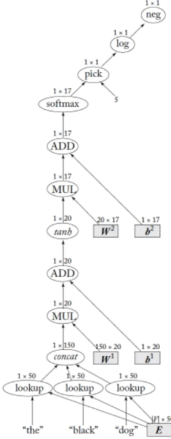
In Figure 2.6, we see the computation graph for a MLP with one hidden-layer and a softmax output transformation. This MLP takes as input three words (e.g. the black dog), converts them into the embedding vector x (using the

embetting matrix E as explained in the previous chapter in section 1.2) and

predicts the part-of-speech tag for the third word (noun is the expected output

(42)

2 Feedforward Neural Networks NNMLP1(x) = y h1 =tanh(xW1+b1) y=sof tmax(h1W2+b2) x∈_R150_,_y_∈ R17 W1 ∈_R150×20,b1 ∈_R20,W2 ∈_R20×17,b2 ∈_R17 Θ = W1,W2,b1,b2

The computation graph also includes one more node pick, which is responsible for selecting the entry corresponding to the true part-of-speech tag (nounin this

example) of the output vectory, which contains the probability distribution over

17 part-of-speech tags (nounis in position 5).

Regardless the apparent complexity of this example, the process for building computation graph is actually very quick and easy by using dedicated software libraries and APIs.

Best Practices for Training Deep Models

Training a neural network is a very hard task from an optimization point view. Firstly, the optimization problem is not convex and so optimization theory does not guarantee us convergence to a global minimum. What happens in practice is that the optimization algorithm produces different results for different (random and small) parameter initialization settings. For this reason it is common to train in parallel different neural networks with different parameter initializations and eventually choose the one which has the best performance of the development set. This procedure is known asrandom restarts. This implies that since different models have been trained, the final prediction on a specific task can be now based on themodel ensembles, e.g. using the rule of majority vote.

Another issue with very deep models is the number hidden layers and param-eters, which causes problems when computing the gradient at the first hidden layers. In this case the backpropagation algorithm suffers from either vanishing (almost 0) or exploding (very large value) gradient.

It can also happen that layers with tanh and sigmoid activations become satu-rated, i.e. these neurons produce output values which are all close to 1 and so the gradient becomes very small. This has a negative effect on the network training, since the saturated neuron is not contributing to the learning algorithm. At this

(43)

point one could change activation function, e.g. ReLu, which prevents neurons from “saturating”, but this introduces the problem of “dead” neurons.

Finally, training deep models has become challenging also from a time and computational point of view. In modern deep learning applications not only it is crucial to choose a fast-convergence optimization algorithm, e.g. SGD, but also it is required fine-tune hyperparameters such as learning rate and minibatch size. A common practice used in the deep learning community to speed up neural network training is to use the parameter initialization of pre-trained models (e.g. word embeddings).

(44)

(45)

3 RNN Models

Recurrent Neural Networks (RNNs) are specialized neural network architectures for processingsequential datax1:n1. As already mentioned in Chapter 2, RNNs

are a class of ANNs which present cycles in their compuational graph.

The main peculiarity of RNNs in the context of NLP is the ability to share parameters Θ across different parts of the network. Such parameter sharing scheme enhances not only the flexibility of the neural network, i.e. the model can be applied to examples of different lenghts, but also the generalization ability of the model, i.e. the model provides good results also for previously unseen instances.

If we think about the variability of natural language data, it is extremely impor-tant to have a flexible model which is able to recognize a particular information regardless its absolute position in the sentence. For example, “Yesterday, it was sunny” and “It was sunny yesterday” should be understood as

sen-tences with the same meaning regardless the position of word yesterdayin the

sentence.

The first goal of this chapter (see section 3.1) is to define RNNs high-level abstraction and to visualize RNNs graphical representation in both folded and unfolded versions. This will then shed the light on the most popular concrete RNN architectures, i.e. Simple RNNs (section 3.2) and Gated RNNs (section 3.3), which have been developed with the aim both to avoid vanishing gradient problems and to model long-range dependencies. Section 3.4 will examine other two RNN architectural variations, i.e. bidirectional RNNs and deep RNNs, which have become popular for solving some specific NLP taks.

The high flexibility of RNNs made it possible to exploit RNNs’ output as the input for other components in a bigger model pipeline architecture. At the end of section 3.4, we will provide an example of RNNs used as Feature Extractor for a PoS Tagging task.

The structure, the examples and related figures of this chapter are mostly taken from Goldberg (2017), in order to be coherent with the notation used in

1_{Keep in mind the difference of notation between}_x

[1], . . . ,x[n] (enumerating the nelements

(46)

3 RNN Models

the previous chapters. A useful source for visualizing and understanding the vanishing gradient problem in RNNs has been Graves (2012). For the sake of clarity for Chapter 4, the notation of gated architectures has slightly changed from Goldberg (2017).

3.1 RNN Abstraction

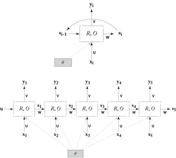
Let x1:n be a sequence of n vectors x1,x2, . . . ,xn, where each xi ∈ Rdin. Our goal is to produce an output vectoryn ∈Rdout 2 using the RNN function

yn =RNN(x1:n) (3.1)

which means that a vector yi is produced for each prefix x1:i of sequence x1:n.

So, the output sequencey1:n can be expressed through the RNN∗ function

y1:n = RNN∗(x1:n)

= RNN(x1),RNN(x1:2), . . . ,RNN(x1:i), . . . ,RNN(x1:n)

= y1,y2, . . . ,yi, . . . ,yn

wherexi ∈Rdin,yi ∈Rdout for all i= 1, . . . , n.

Note that such formulation provides RNNs with a mathematical framework for conditioning on the entire history x1:i when predicting yi. This is in contrast

with the traditionalMarkovian assumption, which assumes a fixed-size window of past dependence and thus does not allow flexibility, which is actually required for many NLP tasks.

Looking more carefully at equation 3.1, the RNN function operates in two steps to produce outputyi:

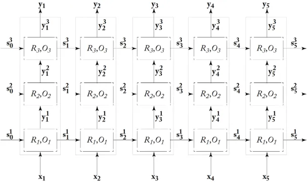
si = R(si−1,xi) (3.2)

yi = O(si) (3.3)

where the RNN first applies function R(·) to a state vector si−1 (containing

the historyx1:i−1) and to the new input vector xi and returns as output a new

state vectorsi3. The second step is to apply the function O(·) to the previously

obtained state vector si and finally obtain the output yi, which is then used for

further prediction.

2_{The subscript}_n_{means that}_y

n has been computed based on the whole sequencex1:n.

3_{Note that it is conventional to start the recursion with an initial state vector}_s

0.

(47)

3.1 RNN Abstraction

Figure 3.1: Recursive (top) and Unfolded (bottom) RNN abstraction.

Looking at equation 3.2, we can notice an interesting recursion

si = R(si−1,xi) = R(R(si−2,xi−1) | {z } si−1 ,xi) ... = R(R(. . .(R(s0,x1) | {z } s1 ,x2). . .),xi) (3.4)

where each new state vector si is obtained as combination of the same

func-tion R(·) applied recursively to different inputs. Moreover, also the output yi is

obtained using always the same function O(·).

This recurrent formulation is the key part to understand how RNNs implement suchparameter sharing mechanism at different time steps.