Central Washington University
ScholarWorks@CWU
All Graduate Projects
Graduate Student Projects
Fall 2017
Visual Data Mining
syeda sadiya
[email protected]Follow this and additional works at:
https://digitalcommons.cwu.edu/graduate_projects
Part of the
Computer and Systems Architecture Commons
Recommended Citation
1. Wrolstadt, Jay: Satellite Smashes Terabyte Data Barrier, NewsFactor Sci::Tech,http://sci.newsfactor.com/perl/story/18424.html, June 2002. 2. Wolfgang Muller,Heidrun Schumann,"Visual Data Mining", NORSIGD Info,2002. 3. Kovalerchuk, B. (2014). Visualization of multidimensional data withcollocated paired coordinates and general line coordinates. In Proc. SPIE 9017,
visualization and data analysis (p. 90170I). 4. O. L. Mangasarian and W. H. Wolberg: "Cancer diagnosis via linearprogramming", SIAM News, Volume 23, Number 5, September 1990, pp 1&18. 5. William H. Wolberg and O.L. Mangasarian: "Multisurface method of patternseparation for medical diagnosis applied to breast cytology",Proceedings of the National Academy of Sciences, U.S.A., Volume 87,December 1990, pp 9193-9196. 6. David J. Slate Odesta Corporation; 1890 Maple Ave; Suite 115; Evanston, IL 60201, David J. Slate ([email protected]) (708) 491-3867, January, 1991 7. H. T. Kahraman, Sagiroglu, S., Colak, I., Developing intuitive knowledgeclassifier and modeling of users’ domain dependent data in web, Knowledge Based Systems, vol. 37, pp. 283-295, 2013. 8. Kovalerchuk B, Grishin V. Adjustable general line coordinates for visualknowledge discovery in nD data. Information Visualization.
VISUAL DATA MINING
A Project Presented to The Graduate Faculty Central Washington University
In Partial Fulfillment
of the Requirements for the Degree Master of Science
Computational Science
by Syeda Sadiya 06 December 2017
ABSTRACT
Occlusion is one of the major problems for interactive visual knowledge discovery and data mining in the process of finding patterns in multidimensional data.This project proposes a hybrid method that combines visual and analytical means to deal with occlusion in visual knowledge discovery called as GLC-S which uses visualization of n-D data in 2D in a set of Shifted Paired Coordinates (SPC). A set of Shifted Paired Coordinates for n-D data consists of n/2 pairs of common Cartesian coordinates that are shifted relative to each other to avoid their overlap. Each n-D point A is represented as a directed graph A* in SPC, where each node is the 2D projection of A in a respective pair of the Cartesian coordinates.
The proposed GLC-S method significantly decrease cognitive load for analysis of n-D data and simplify pattern discovery in n-D data. The GLC-S method iteratively splits n-D data into non-overlapping clusters (hyper-rectangles) around local centers and visualizes only data within these clusters at each iteration. The requirements for these clusters are to contain cases of only one class and be the largest cluster with this property in SPC visualization.
Such sequential splitting allows: (1) avoiding occlusion, (2) finding visually local classification patterns, rules, and (3) combine local sub-rules to a global rule that classifies all given data of two or more classes. The computational experiment with Wisconsin Breast Cancer data(9-D), User Knowledge Modeling data(6-D), and Letter Recognition data(17-D) from UCI Machine Learning Repository confirm this capability. At each iteration, these data have been split into training (70%) and validation (30%) data. It required 3 iterations in Wisconsin Breast Cancer data, 4 iterations in User Knowledge Modeling and 5 iterations in Letter Recognition data and respectively 3, 4, 5 local sub-rules that covered over 95% of all n-D data points with 100% accuracy at both training and validation experiments. After each iteration, the data that were used in this iteration are removed and remaining data are used in the next iteration. This removal process helps to decrease occlusion too. The GLC-S algorithm refuses to classify remaining cases that are not covered by these rules, i.e.,., do not belong to found hyper-rectangles. The interactive visualization process in SPC allows adjusting the sides of the hyper-rectangles to maximize the size of the hyper-rectangle without its overlap with the
hyper-rectangles of the opposing classes.
The GLC-S method splits data using the fixed split of n coordinates to pairs. This hybrid visual and analytical approach avoids throwing all data of several classes into a visualization plot that typically ends up in a messy highly occluded picture that hides useful patterns. This approach allows revealing these hidden patterns.
The visualization process in SPC is reversible (lossless). i.e.,., all n-D information is visualized in 2D and can be restored from 2D visualization for each n-D case. This hybrid visual analytics method allowed classifying n-D data in a way that can be communicated to the user’s in the understandable and visual form.
ACKNOWLEDGEMENT
Guidance, help, and motivation are the vital bricks in the construction of a research work. I would like to extend my gratitude to everyone who has helped me in this work.
I would like to express my deep sense of gratitude and special thanks to my advisor Dr. Boris Kovalerchuk, who gave me this opportunity to work on this project. His valuable suggestions, timely guidance, continuous support, motivation, and immense knowledge helped me doing a lot in this project and I learned so many new things I am really thankful to him. It would not have been possible for me to proceed, but his motivation and encouragement made me do so.
I would like to thank my committee members Dr. Razavan Andonie and Dr. Christos Graikos for their time to see my work and provide suggestions.
I would like to thank all the faculty members in the Department of Computer Science for their extended support when I was in need.
I take this opportunity to express my sincere gratitude and thanks to my beloved Parents, Husband, and Brothers for their moral support and kind cooperation throughout my work.
TABLE OF CONTENTS
C
HAPTER
1 INTRODUCTION 1
2 LOSELESS VISUALIZATION OF n-D DATA 3 3 SHIFTED PAIRED COORDINATE (SPC) 4
4 LITERATURE REVIEW 7
5 DATASET DESCRIPTION 9
6 EXPERIMENTAL STEPS OF THE SAMPLE 10
7 EXPERIMENTAL RESULTS 16
7.1 User Knowledge Modeling Dataset (UKM) . . . 17 7.2 Wisconsin Breast Cancer Dataset(WBC) . . . 24 7.3 Letter Recognition Dataset(LR) . . . 30
8 SOFTWARE DESCRIPTION 53
9 CONCLUSION 54
L
IST OF
T
ABLES
7.1 Number of samples in Iteration 1 . . . 17
7.2 Number of samples in Iteration 2 . . . 17
7.3 Number of samples in Iteration 3 . . . 17
7.4 Remaining samples in UKM . . . 18
7.5 Values of centers in UKM . . . 18
7.6 Values of thresholds in UKM . . . 18
7.7 Confusion Matrix for testing phase in WBC . . . 19
7.8 Number of cases in Iteration 1 . . . 24
7.9 Number of cases in Iteration 2 . . . 24
7.10 Number of cases in Iteration 3 . . . 24
7.11 Remaining cases in WBC . . . 24
7.12 Values of centers in WBC . . . 25
7.13 Values of thresholds in WBC . . . 25
7.14 Confusion Matrix for testing phase in WBC . . . 26
7.15 Number of instances in Iteration 1 . . . 30
7.16 Number of instances in Iteration 2 . . . 30
7.17 Number of instances in Iteration 3 . . . 30
7.18 Number of instances in Iteration 4 . . . 30
7.19 Number of instances in Iteration 5 . . . 31
7.20 Remaining cases in LR(AB,C) . . . 31
7.21 Values of centers in LR(AB,C) . . . 31
7.22 Values of thresholds in LR(AB,C) . . . 32
7.23 Confusion Matrix for testing phase in LR(AB,C) . . . 32
7.24 Number of instances in Iteration 1 . . . 39
7.25 Number of instances in Iteration 2 . . . 39
7.26 Number of instances in Iteration 3 . . . 39
7.27 Remaining cases in LR(A,B) . . . 39
7.28 Values of centers in LR(A,B) . . . 40
7.29 Values of thresholds in LR(A,B) . . . 41
7.30 Confusion Matrix for testing phase in LR(A,B) . . . 41
7.31 Number of instances in Iteration 1 . . . 44
7.32 Number of instances in Iteration 2 . . . 44
7.33 Number of instances in Iteration 3 . . . 44
7.34 Number of instances in Iteration 4 . . . 44
7.35 Number of instances in Iteration 5 . . . 44
7.36 Remaining cases in LR(T,I) . . . 45
7.37 Values of centers in LR(T,I) . . . 45
7.38 Values of thresholds in LR(T,I) . . . 46
L
IST OF
F
IGURES
3.1 a) Point (5,10) is produced by adding (2,2) to (3,8) in SPC b) 6-D points
in SPC . . . 5
3.2 a) SPC with 3 cartesian coordinates b)The same 6-D points as above in Parallel Coordinates . . . 5
6.1 Sample Data . . . 10
6.2 Duplicating the last column of the data . . . 10
6.3 Normalized data . . . 11
6.4 Training Data . . . 11
6.5 Testing Data . . . 12
6.6 Data from class Middle . . . 12
6.7 Data from class High . . . 12
6.8 Data from class Low . . . 13
6.9 Data from class Very Low . . . 13
6.10 Median calculation for each column . . . 13
6.11 Distance calculation for each row . . . 14
6.12 Minimum of the euclidean distances . . . 14
6.13 Row with minimum distance . . . 14
6.14 Subtracted rows from row having minimum distance . . . 15
6.15 Rows that falls within the threshold . . . 15
6.16 Consolidated Training and Testing data . . . 15
7.1 Training results of UKM in iteration 1 . . . 20
7.2 Testing results of UKM in iteration 1 . . . 20
7.3 Training results of UKM in iteration 2 . . . 21
7.4 Testing results of UKM in iteration 2 . . . 21
7.5 Training results of UKM in iteration 3 . . . 22
7.6 Testing results of UKM in iteration 3 . . . 22
7.7 Remaining records of class High, VeryLow in training . . . 23
7.8 Remaining records of class High, VeryLow in testing . . . 23
7.9 Training results of WBC in iteration 1 . . . 27
7.10 Testing results of WBC in iteration 1 . . . 27
7.11 Training results of WBC in iteration 2 . . . 28
7.12 Testing results of WBC in iteration 2 . . . 28
7.13 Training results of WBC in iteration 3 . . . 29
7.14 Testing results of WBC in iteration 3 . . . 29
7.15 Remaining records of class Malignant in training . . . 29
7.16 Remaining record of class Malignant in testing . . . 29
7.17 Training results of LR(AB,C) in iteration 1 . . . 33
7.18 Testing results of LR(AB,C) in iteration 1 . . . 33
7.19 Training results of LR(AB,C) in iteration 2 . . . 34
7.20 Testing results of LR(AB,C) in iteration 2 . . . 34
7.21 Training results of LR(AB,C) in iteration 3 . . . 35
7.22 Testing results of LR(AB,C) in iteration 3 . . . 35
7.23 Training results of LR(AB,C) in iteration 4 . . . 36
7.24 Testing results of LR(AB,C) in iteration 4 . . . 36
7.25 Training results of LR(AB,C) in iteration 5 . . . 37
7.27 Remaining instances of class AB in training . . . 38
7.28 Remaining instances of class C in training . . . 38
7.29 Remaining instances of class AB in testing . . . 38
7.30 Remaining instances of class C in testing . . . 38
7.31 Training results of LR(A,B) in iteration 1 . . . 42
7.32 Testing results of LR(A,B) in iteration 1 . . . 42
7.33 Training results of LR(A,B) in iteration 2 . . . 42
7.34 Testing results of LR(A,B) in iteration 2 . . . 42
7.35 Training results of LR(A,B) in iteration 3 . . . 42
7.36 Testing results of LR(A,B) in iteration 3 . . . 42
7.37 a)Remaining instances of class A in training . . . 43
7.38 b)Remaining instances of class B in training . . . 43
7.39 a)Remaining instances of class A in testing . . . 43
7.40 b)Remaining instances of class B in testing . . . 43
7.41 Training results of LR(T,I) in iteration 1 . . . 47
7.42 Testing results of LR(T,I) in iteration 1 . . . 47
7.43 Training results of LR(T,I) in iteration 2 . . . 48
7.44 Testing results of LR(T,I) in iteration 2 . . . 48
7.45 Training results of LR(T,I) in iteration 3 . . . 49
7.46 Testing results of LR(T,I) in iteration 3 . . . 49
7.47 Training results of LR(T,I) in iteration 4 . . . 50
7.48 Testing results of LR(T,I) in iteration 4 . . . 50
7.49 Training results of LR(T,I) in iteration 5 . . . 51
7.50 Testing results of LR(T,I) in iteration 5 . . . 51
7.51 a)Remaining instances of class T in training . . . 52
7.52 b)Remaining instances of class I in training . . . 52
1 INTRODUCTION
The amount of data in both public and private sectors is increasing at a very rapid scale. If this information is not analyzed to derive useful insights prompting for positive reinforcement, all this data generated will be of no value. The siloed approach of using visual representation to derive insights and advanced data mining techniques to wrangle the data has always been a challenge. The challenge is that they represent part of the information in the best way possible they can, making it hard to derive true insights. This limitation is overcome in my project, here I combine the data mining algorithm to do advanced analytics and at the same time visualize it to achieve an easy consumption.
Since human eyes are not susceptible to analyze a large amount of abstract numeric data and find the hidden patterns associated with them, we need enhanced
visualization tools to represent the data in 2D losslessly. Hence, this project is devoted to overcome these inabilities and provide user-friendly visualizations. While there are numerous data visualization techniques available for visualizing the data in graphical formats such as bar charts, heat maps etc., but these tools have very limited capabilities to overcome the challenges faced by humans as they can be applied to relatively smaller datasets and dimensions. One of the major motivations for the emergence of visual analytics research to develop 2D visualization of the data is due to the inability to find patterns associated with n-D data by naked eyes. While many visual analytical techniques have been evolved they will not suffice to restore and represent the n-D of the data completely in 2D space i.e.,., lossy
representation of data and this will give rise to challenges in visualization[9]. In this project, we have presented ways to overcome the limitations in analyzing large data with complex patterns.
Data mining strategies are generally applied to thought fully collected data and frequently focus on the exploring of structures for which a valid data analysis is very appropriate and quite likely to yield insights. The goal of this project is to improve the accuracy of predictive classification of datasets using the approach called General Line Coordinates (GLC) with its subclass Shifted Paired Coordinated (SPC)[3]. "GLC is drawing ’n’ coordinate axes in 2D in a variety of ways: parallel, shifted, collocated etc. The data collected are often multidimensional and discovering patterns in big multidimensional data using visual means is a
long-standing problem in Information Visualization, Visual Analytics, Visual Data Mining, and Data Science in general"[10].
Reducing the data from high dimensionality to a meaningful representation of low dimensionality will often increase the efficiency of the algorithm, but it might not preserve the n-D informational of the data fully. To mitigate this we use GLC and SPC as they provide a framework using which data miners can perform an intuitive assessment and have a precise evaluation on a large number of visual
GLC with its subclass SPC altogether extends an arrangement of lossless facilitate frameworks. GLC contain an infinite number of coordinate systems. GLC permit preserving:
1. reversible (coordinated) mapping between n-D data and their 2D portrayals and
2. the similarity of n-D points in their 2D visual portrayals
The principle inspiration for lossless GLC is saving all n-D information in 2D visualization,i.e.,., the capacities to reestablish every n-D point totally from its 2D visual portrayal that is helpful and critical in Visual Analytics and Machine
Learning[8].
This report is organized as follows. Chapter 2 presents the concept of lossless visualization of n-D data. Chapter 3 provides overview of SPC. Chapter 4 provides literature review. Dataset description is described in Chapter 5. Chapter 6 provides details of the experimental steps. Experimental results are discussed in Chapter 7. Chapter 8 provides the software details and Conclusion is presented in Chapter 9.
2 LOSELESS VISUALIZATION OF
N
-D DATA
This project depicts the proposed new algorithms for lossless visual representation of high-dimensional information and their associations with human difficulties.
One of the ideas of lossless GLC method is called Parallel Coordinates (PC). In PC, we draw every coordinate axes in 2D located one after another on ’s’ single straight lines as shown in Figure 3.2b). Despite the fact that it is an extremely well-known visualization technique to preserve the n-D data, it is not adequate to address visualization difficulties of all possible datasets such as occlusion that is basic for larger datasets. To mitigate this we utilize more enhanced visualization called SPC. The project concentrates on Shifted Paired Coordinates as a subset of General Line Coordinates. The benefits of these coordinates have been demonstrated both mathematically and on the data. These focal points manage future investigations to comprehend a noteworthy challenge. This challenge is discovering conditions for a provable property of more straightforward and less covered lossless 2D
representation of the non-overlapping hyper-rectangles in n-D[9].
The benefit of a wide class of GLC is that it permits numerous distinctive
representations of similar data with the diverse perceptual and cognitive attributes. This variety expands the odds that humans will have the capacity to uncover the shrouded n-D designs in these visualizations. It isn’t reasonable to expect that a solitary representation will do this for every single conceivable data and all humans.A full characterization of the general line coordinates for the cognitively effective n-D data representation is an errand for future research and also the more profound connections with Machine Learning figuring out how to have the capacity to build visually the learning algorithms utilizing visual means in GLC. This is a zone of future investigations for the plan of more complete procedures and for expanding to other data mining/machine algorithms learning strategies[9].
For example, assume that we have established that new data have the same mathematical structure that was explored before. Then we can use the derived matched structural properties. Consider n-D data with a mathematical structure where all n-D points of class C1 are in the hypercube H1 and all n-D points of class C2 are in another hypercube H2 and the separation between these hypercubes is greater than or equivalent to k lengths of these hypercubes.Assume that it was established mathematically that for any n-D data with this structure a lossless visualization method V1, produces visualizations of n-D vectors of classes C1 and C2 that don’t overlap in 2-D. Next, assume that this property was tried on new n-D information and affirm. For this situation, we can apply visualization method V1 with certainty that it will deliver attractive perception without overlapping of two classes. Additionally, if the basic property is negative in capacity to visualize the patterns without overlapping then this will prompt the conclusion that the method should not be used for the given information[9].
3 SHIFTED PAIRED COORDINATE (SPC)
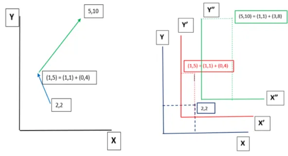
Basic Shifted Paired Coordinate shows every next pair in the shifted coordinate system. SPC is a process of drawing each next pair in the shifted paired coordinate system by adding (1,1) to the second pair, (2,2) to the third pair, (i-1,i-1) to the i-th pair, and so on and so on. Generally, SPC allows shift to any given pair of numbers.
A set of Shifted Paired Coordinates for n-D data consists of n/2 pairs of common Cartesian coordinates that are shifted relative to each other to avoid their overlap. Each n-D point A is represented as a directed graph A* in SPC, where each node is the 2D projection of A in a respective pair of the Cartesian coordinates.
The main steps in implementing SPC are:
• Normalizing all the dimensions to some interval, e.g., [0, 1];
• Grouping attributes into consecutive pairs (x, y) (x’, y’) (x", y");
• Plotting each pair in the same orthogonal normalized Cartesian coordinates X and Y;
• Plotting a directed graph (x, y) ->(x’, y’) -> (x", y") with directed paths from (x, y) to (x’, y’) and from (x’, y’) to (x", y").
Let us consider an example to represent n-D data in 2D space using lossless SPC. Here for this example, we can use a state vector X = (X, Y, X’, Y’, X", Y") as (2,2,0,4,3,8).
Figure 3.1a) shows the application of SPC to (2,2,0,4,3,8) with the directed graph drawn as two arrows: from (2,2) to (0, 4) and from (0, 4) to (3,8).
• The first pair (2,2) is drawn in the (X, Y) system.
• The next pair (0,4) is drawn not in the original system X, Y), but in the shifted coordinate system denoted as (X’, Y’), where coordinate X is shifted up by 1, and coordinate Y is shifted towards right by 1. This means that the pair (0, 4) in coordinates (X’, Y’) will be a pair (0, 4) + (1.1) = (1, 5) in the original
coordinates (X, Y).
• The next pair (3,8) is drawn in the (X", Y") coordinates.
• For the points (2,2,0,4,3,8), the arrows are drawn from (2,2) to (1, 1)+(0, 4) = (1, 5) then from (1, 5) to (2, 2) + (3,8) = (5,10) see Figure 3.1a).
Figure 3.1b) shows in detail how we can plot the same 6-D points in SPC. X is shifted by 1 towards up and y is shifted by 1 towards right for every next pair of points.
Figure 3.1: a) Point (5,10) is produced by adding (2,2) to (3,8) in SPC b) 6-D points in SPC
The same points can be plotted in SPC using three cartesian coordinates as shown in Figure 3.2a) (2,2) is drawn in the first cartesian coordinate (x,y), (0,4) is drawn in the second cartesian coordinate (X’,Y’) and (3,8) is drawn in the third cartesian coordinate(X", Y").
Figure 3.2b) shows how the same points can be plotted using Parallel
Coordinates(PC). But in PC, no n-D point can be represented as a solitary 2D point with such preserved n-D vicinity. This property essentially disentangles the visual pattern of the n-D data class and profoundly improves the capacities to find n-D classes visually utilizing their 2D SPC representations alongside two times less occlusion than for graphs in PC.
Figure 3.2: a) SPC with 3 cartesian coordinates b)The same 6-D points as above in Parallel Coordinates
Shifted Paired Coordinate is a visual approach to execute outlining a complex non-linear transformation of the n-D data space into another space where a
hyper-rectangle can be drawn for n-D data classification which we will see in the experimental results in chapter 7.
4 LITERATURE REVIEW
Wisconsin Breast Cancer(WBC)
There has been a lot of research on medical diagnosis of breast cancer with WBCD in literature, and most of them reported high classification accuracies. In [15], a learning algorithm that combined logarithmic simulated annealing with the perceptron algorithm was used and the reported accuracy was 98.8%. In [16], the classification technique used fuzzy-GA method reaching a classification accuracy of 97.36%. In Setiono (2000), the classification was based on a feed-forward neural network rule extraction algorithm. The reported accuracy was 98.10%.
(Quinlan)[17] reached 94.74% classification accuracy using 10-fold cross-validation with C4.5 decision tree method. (Hamiton, Shan, & Cercone, 1996 )[18] obtained 94.99% accuracy with RIAC method, while (Ster & Dobnikar)[19] obtained 96.8% with linear discreet analysis method. In Abonyi and Szeifert[20], an accuracy of 95.57% was obtained with the application of supervised fuzzy clustering technique. In Polat and Gunes [21], least square SVM was used and an accuracy of 98.53% was obtained. In Akay ME[14], SVM and feature selection was used and an accuracy of 99.02% for the 70-30% was achieved[14].
Letter Recognition(LR)
Adnan Alrabea et.al [22] uses Principal Component Analysis (PCA) for generating the first principal component for initializing the centroid for k-means clustering. Initially, the principal components in the dataset are gathered using PCA. From the obtained components, the first principal component is used for initializing the cluster centroid. It has a better accuracy. Different methods have been proposed by combining PCA with k-means for high dimensional data set. But the accuracy of the k-means clusters heavily depending on the random choice of initial centroids[13].
Fahim A M et al.[23] proposed an efficient method for assigning data points to clusters. In this, the distance between data points and all the centroids are computed for each iteration. The distance function is calculated based on
Euclidean Distance and another one based on a heuristic to reduce the number of distance calculations. The main drawback of this method is that the initial centroids are determined randomly which in turn increases complexity[13].
Dhanbal[13] proposed a method that first, applied PCA to reduce the
dimensionality of the given dataset, then applied k-MAM method to find the initialization and using the initial centroids, he used normal kmeans algorithm for finding the clusters. The highest accuracy obtained in the classification was 96%.
User Knowledge Modeling(UKM)
Kahraman [25] and Martins et al. [26] reported that considering the historical data of the users during user modeling process makes a significant contribution to efficiencies of the models and the success during teaching/learning process while the users are registering to the system in AEEC, they declare their previous
experiences. The users fill in an information form about whether they joined such a course before and if so whether they succeed or not. Depending on the previous experiences and knowledge of the users, the user modeling system picks the suitable one amongst various user modeling strategies. In this regard, the user modeling strategy in AEEC is adaptable [25,24].
In literature, although there are many approaches developed for modeling the user knowledge, it is seen that most of them are not used for real-world applications. The basic reasons of this problem turn out to be the dependency of the developed user modeling approaches to the application domain, their complexity, their processes, their focuses on the subject of theoretic modeling (inability of applicability) and also only few of them have been tested by real data sets [26]. According to the literature, each of the users’ features is equally important to measure the distances among them [27,28,29,30].This is one of the main causes of misclassification in knowledge modeling. Therefore, the importance or weight values of users’ features on their knowledge class should be determined. Consequently, a
domain-independent object model, a classification method suitable for user modeling tasks should be developed[24].
In [24],presents a powerful, efficient and simple,Intuitive Knowledge Classifier method successfully and proposes to model the domain dependent data of users. A domain independent object model, the user modeling approach and the
weight-tuning method were combined with instance-based classification algorithm to improve classification performances of well-known the Bayes and the k-nearest neighbor-based methods.
The experimental studies have shown that the weighting of domain dependent data of students and combination of user modeling algorithms and population-based searching approach play an essential role in classifying performance of user modeling system. The proposed system improves the classification accuracy of instance-based user modeling approach for all distance metrics and different k-values. Intuitive weighting method improves the classification accuracy of instance-based knowledge classifier for all distance metrics and different k-values. The proposed method has achieved an average classification accuracy of 97.5% [24].
5 DATASET DESCRIPTION
1. Wisconsin Breast Cancer Dataset(WBC)
The WBC dataset is taken from the UCI machine learning repository in our experiments. This dataset is commonly used by researchers who use machine learning methods for breast cancer classification, so it provides us to compare the performance of our method with that of others. The dataset contains total 699 samples among which 16 contains missing values. The 683 samples taken for the experiment consists of nine features, each of which is represented as an integer between 1 and 10. The features are; clump thickness (F1), uniformity of cell size (F2), uniformity of cell shape (F3), marginal adhesion (F4), single epithelial cell size (F5), bare nucleoi (F6), bland chromatin (F7), normal nuclei (F8), and mitoses (F9). 444 samples of the dataset belong to benign class, and the rest 239 are of malignant class [4,5].
2.Letter Recognition Dataset(LR)
Letter recognition dataset is taken from UCI machine repository dataset [6]. The objective is to identify each of many black-and-white rectangular pixel displays as one of the 26 capital letters of the English alphabet. The character images were based on 20 different fonts and each letter within these 20 fonts was randomly distorted to produce a file of 20,000 unique stimuli. Each stimulus was converted into 16 primitive numerical attributes (statistical moments and edge counts) which were then scaled to fit into a range of integer values from 0 through 15. For the better analysis, we have chosen 2291 instances with 17 attributes to identify the letters A, B and C[6].
3.User Knowledge Modeling Dataset(UKM)
User Knowledge Modeling is the real dataset about the student’s knowledge status about the subject of electrical dc machines. The user’s knowledge class was
classified by the author using the intuitive knowledge classifier k-nearest algorithm. This dataset has multivariate characteristics. This data contains total 403 data samples which have four type of classes namely Very Low (50), Low (129), Medium (122) and High (130) [7].
There is no missing value in the dataset and it has five attributes given as: 1. STG (The degree of study time for goal object materials),
2. SCG (The degree of repetition number of user for goal object materials)
3. STR (The degree of study time of user for related objects with goal object)
4. LPR (The exam performance of user for related objects with goal object)
5. PEG (The exam performance of user for goal objects)
6 EXPERIMENTAL STEPS OF THE SAMPLE
1. Consider n-D dataset X. Here I’m using a sample dataset with 14 records having 5 classes.
Figure 6.1: Sample Data
2. Check if X has even number of columns because in SPC to maintain uniformity and relation between the coordinates we need to have an even number of columns in the dataset. If not, duplicate one of the columns as shown in Figure 6.2. Each column is considered as a coordinate e.g. x1, x2, x3, x4 etc.
3. Normalize the data column-wise in the range [0,1] as shown in Figure 6.3.
Zi=(x−mi n(x))/(max(x)−mi n(x)) (6.1)
Where,Zi = normalized data, x = column
Figure 6.3: Normalized data
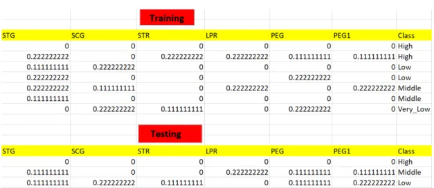
4. Split the normalized dataZi as training and testing e.g in the ratio 70:30 as
shown in Figure 6.4 and Figure 6.5.
Figure 6.5: Testing Data
5. Divide the data according to the class. Here in this example, I have 4 classes namely: High, Middle, Low, Very Low. Hence I’m dividing them separately from both training and testing.
Figure 6.6: Data from class Middle
Figure 6.8: Data from class Low
Figure 6.9: Data from class Very Low
6. Calculate the median of each column in each class as shown in the Figure 6.10.
Mi=med i an(x1:Xn) (6.2)
where,X1= first element of the column, Xn= last element of the column.
Figure 6.10: Median calculation for each column
7. Calculate the square root of distance between the median of each column and every element of the row.
Di=
q
(M1−An)2+(M2−Bn)2+(M3−Cn)2+(M4−Dn)2+(M5−En)2+(M6−Fn)2
(6.3) Where,M1,M2,M3,M4,M5,M6- median of column 1,2,3,4,5,and 6.
Figure 6.11: Distance calculation for each row
8. Find the minimum of the distances calculated in step 7 and select the complete row corresponding to the minimum distance.
Mi n=mi ni mum(Di) (6.4)
Figure 6.12: Minimum of the euclidean distances
Figure 6.13: Row with minimum distance
9. Subtract each row by the minimum distance row selected in step 8. In the below Figure 6.14 the rows of class High have been subtracted from the selected row.
Figure 6.14: Subtracted rows from row having minimum distance
10. Choose a thresholdTi and check if each and every value in the row falls within
the thresholdTi. If yes, then choose the row if not reject it.
Figure 6.15: Rows that falls within the threshold
11. Once all the rows have been chosen from all the classes of training and testing data separately, consolidate them.
Figure 6.16: Consolidated Training and Testing data
12. Plot them using SPC. The median’s from each class can be used as a center to visualize the data of that particular class around them.
7 EXPERIMENTAL RESULTS
• To evaluate the effectiveness of our method, we have conducted the
experiment on three datasets described in chapter 5 and in every experiment we have used the same experimental steps discussed in chapter 6.
• We have conducted multiple iterations on each dataset. For testing data we always use center n-D points and thresholds from the training.
• The threshold is evaluated for all the coordinates x1,x2,x3 etc.,. and we build hyper-rectangles.
• Accuracy Calculation:
This is the percentage of a number of records that are perfectly classified by the total number of records. Accuracy discovers the one-to-one relationship between clusters and classes and measures the extent to which each cluster contains data points from the corresponding class.
A=Mi/Ti (7.1)
where,Mi = total number of perfectly classified records Ti=total number of records
The goals of this experiment are:
1. Test effectiveness of the proposed method GLC with SPC for visual discovery of n-D data structures for data with multiple dimensions.
2. Identify the advantages of SPC by experimenting with multiple datasets con-sidering different threshold values for classification.
7.1 U
SERK
NOWLEDGEM
ODELINGD
ATASET(UKM)
In UKM dataset there are 403 samples and 6 attributes. The last attribute is the class and we do not use this for plotting. To make the number of columns even to plot the data in SPC one of attributes of the dataset has been duplicated and we have 6 attributes for plotting.
UKM data has been split into training and testing with 258 and 145 samples. 3 iterations have been performed to cover all the data points.
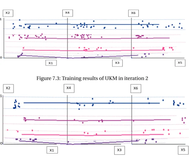
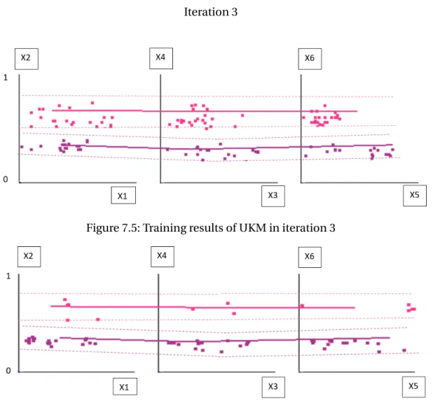
There are 4 classes in the dataset and we have categorized them from top to bottom as:
• High - Class 1, color = blue
• Middle - Class 2, color = magenta
• Low - Class 3, color = pink
• VeryLow - Class 4, color = purple
Training High Middle Low VeryLow
H11 22 0 0 0
H21 0 40 0 0
H31 0 0 38 0
H41 0 0 0 12
Testing High Middle Low VeryLow
H11 15 0 0 0
H21 0 22 0 0
H31 0 0 20 0
H41 0 0 0 12
Table 7.1: Number of samples in Iteration 1
Training High Middle Low VeryLow
H12 40 0 0 0
H22 0 31 0 0
H32 0 0 25 0
H42 0 0 0 11
Testing High Middle Low VeryLow
H12 23 0 0 0
H22 0 7 0 0
H32 0 0 15 0
H42 0 0 0 13
Table 7.2: Number of samples in Iteration 2
Training High Middle Low VeryLow
H23 0 17 0 0
H33 0 0 20 0
Testing High Middle Low VeryLow
H23 0 5 0 0
H33 0 0 11 0
Remaining High Middle Low VeryLow Training 1 0 0 1
Testing 1 0 0 1
Table 7.4: Remaining samples in UKM
Rules of Iteration:
1. R1 : IfX ∈H11∨H12thenX ∈C l ass1 i.e., High
where, X = n-D data.
2. R2 : IfX ∈H21∨H22∨H23thenX ∈C l ass2 i.e., Middle
3. R3 : IfX ∈H31∨H32∨H33thenX ∈C l ass3 i.e., Low
4. R4 : IfX ∈H41∨H42thenX ∈C l ass4 i.e., VeryLow
• Hj k=
©
X: |Cj ki-Xi|≤Tj ki, i=1,2,3,4,5,6
ª
where, j = class, k=iteration, i=coordinate
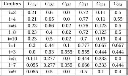
Centers C11i C12i C21i C22i C23i C31i C32i C33i C41i C42i i=2 0.98 0.875 0.57 0.46 0.355 0.25 0.15 0.67 0.0 0.05 i=4 0.975 0.87 0.56 0.455 0.353 0.25 0.15 0.66 0.05 0.0 i=6 0.98 0.875 0.56 0.46 0.355 0.25 0.15 0.662 0.0 0.05 i=1 0.4 0.39 0.3775 0.385 0.35 0.295 0.35 0.67 0.2 0.3 i=3 0.34 0.347 0.3 0.28 0.26 0.39 0.4 0.4 0.3 0.1 i=5 0.4 0.52 0.29 0.72 0.78 0.49 0.59 0.48 0.3 0.13
Table 7.5: Values of centers in UKM
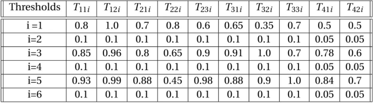
Thresholds T11i T12i T21i T22i T23i T31i T32i T33i T41i T42i
i =1 0.8 1.0 0.7 0.8 0.6 0.65 0.35 0.7 0.5 0.5 i=2 0.1 0.1 0.1 0.1 0.1 0.1 0.1 0.1 0.05 0.05 i=3 0.85 0.96 0.8 0.65 0.9 0.91 1.0 0.7 0.78 0.6 i=4 0.1 0.1 0.1 0.1 0.1 0.1 0.1 0.1 0.05 0.05 i=5 0.93 0.99 0.88 0.45 0.98 0.88 0.9 1.0 0.84 0.7 i=6 0.1 0.1 0.1 0.1 0.1 0.1 0.1 0.1 0.05 0.05
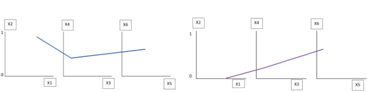
5. The remaining samples in training phase from the class Low is 1 sample and from class High is 1 sample.Hence, the rule can be given as,
R5: If (X=XH1)⇒Class 1.
where, H1 = Remaining sample from the class High R6: If (X=XV L1)⇒Class 4.
where, VL1 = Remaining sample from the class VeryLow
6. The remaining cases in testing phase from the class VeryLow is 1 sample and from the class High is 1 sample. But, in the testing we cannot know in prior which sample belongs to which class like we did in training phase. Hence we augment the rule and draw a confusion matrix to show the refused cases in the testing phase which will not be found within the hyper-rectangles and find the accuracy.
High Middle Low VeryLow Refusal High 38 0 0 0 0 Middle 0 34 0 0 0
Low 0 0 46 0 0
VeryLow 0 0 0 25 0 Refusal 1 0 0 1 0
Table 7.7: Confusion Matrix for testing phase in WBC
Accuracy = 143 / 145 = 98.62%
From the above results we can conclude that using GLC with SPC we have achieved an accuracy of 98.62% which is better than the accuracy of 97.5% in the literature[24].
The results of the iterations are shown in the figures below along with the remaining cases that do not found in the hyper-rectangles during the training and testing
phase.
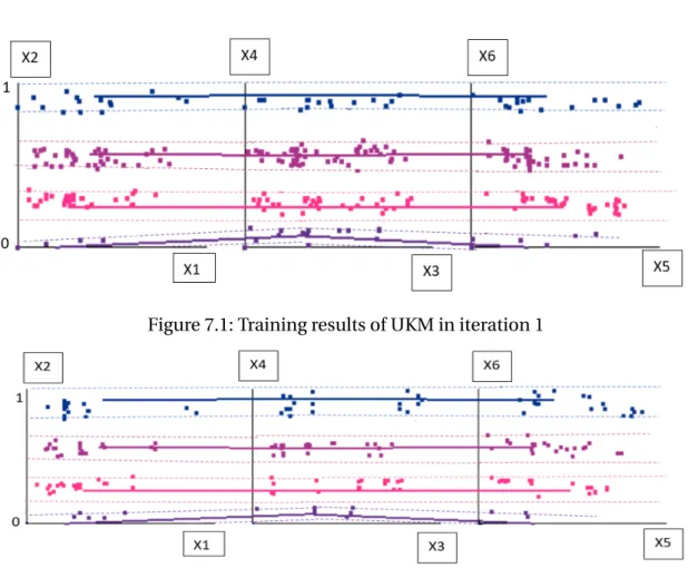
Iteration 1
Figure 7.1: Training results of UKM in iteration 1
Iteration 2
Figure 7.3: Training results of UKM in iteration 2
Iteration 3
Figure 7.5: Training results of UKM in iteration 3
Remaining records
Figure 7.7: Remaining records of class High, VeryLow in training
Remaining records
7.2 W
ISCONSINB
REASTC
ANCERD
ATASET( WBC)
In WBC dataset there are 699 cases and 9 attributes. There are 16 NA values hence those records have been removed and we use 683 cases in the experiment. To make the number of columns even to plot the data in SPC the last attribute of the dataset has been duplicated and we have 10 attributes.
The data are split into the ratio 70:30 i.e., 478 cases in training and 205 cases in testing. There are 170 Malignant and 308 Benign cases in training, 69 Malignant and 136 Benign cases in Testing. There are 2 classes and they have been categorized as:
• Benign - Class 1, color = blue
• Malignant - Class 2, color = red
3 iterations have been performed to cover all the data points. The details of the data points in each iteration are shown in the tables below.
Training Malignant Benign
H11 0 276
H21 128 0
Testing Malignant Benign
H11 0 126
H21 50 0
Table 7.8: Number of cases in Iteration 1
Training Malignant Benign
H12 0 6
H22 26 0
Testing Malignant Benign
H12 0 4
H22 15 0
Table 7.9: Number of cases in Iteration 2
Training Malignant Benign
H13 0 6
H23 30 0
Testing Malignant Benign
H13 0 6
H23 3 0
Table 7.10: Number of cases in Iteration 3
Remaining Malignant Benign Training 6 0
Rules of Iteration:
1. R1 : IfX ∈H11∨H12∨H13thenX ∈C l ass1 i.e., Benign
2. R2 : IfX ∈H21∨H22∨H23thenX ∈C l ass2 i.e., Malignant
• Hj k=
©
X: |Cj ki-Xi|≤Tj ki, i=1,2,3,4,5,6,7,8,9,10
ª
where, j = class, k=iteration, i=coordinate
Centers C11i C12i C13i C21i C22i C23i
i=2 0.21 0.6 0.0 0.72 0.11 0.5 i=4 0.21 0.65 0.0 0.77 0.11 0.55 i=6 0.23 0.66 0.02 0.76 0.123 0.5 i=8 0.23 0.4 0.02 0.72 0.123 0.5 i=10 0.23 0.5 0.02 0.7 0.13 0.4 i=1 0.2 0.44 0.1 0.777 0.667 0.667 i=3 0.0 0.33 0.555 0.555 0.444 0.444 i=5 0.111 0.277 0.0 0.444 0.333 0.0 i=7 0.055 0.277 0.055 0.666 0.333 0.444 i=9 0.055 0.5 0.0 0.5 0.1 0.4
Table 7.12: Values of centers in WBC
Thresholds T11i T12i T13i T21i T22i T23i
i =1 0.8 0.9 0.2 1.0 1.0 1.0 i=2 0.1 0.1 0.05 0.1 0.1 0.1 i =3 0.6 0.8 0.2 1.0 0.5 0.8 i=4 0.1 0.1 0.05 0.1 0.1 0.1 i =5 1.0 0.6 0.1 1.0 1.0 0.2 i=6 0.1 0.1 0.05 0.1 0.1 0.1 i =7 0.8 0.6 0.5 1.0 0.6 0.7 i =8 0.8 0.9 0.05 1.0 1.0 1.0 i =9 0.1 0.6 0.1 0.8 0.1 0.9 i =10 0.8 0.9 0.05 1.0 1.0 1.0
3. The remaining cases in training phase from the class Malignant are 6.Hence, the rule can be given as,
R3: If (X=XM1)∨(X=XM2)∨(X=XM3)∨(X=XM4)∨(X=XM5)∨(X=XM6)⇒
Class 2.
4. The remaining cases in testing consist of single case from the class Malignant. But, in the testing we cannot know in prior which case is benign or malignant like we did in training phase. Hence we augment the rule and draw a
confusion matrix to show the refused cases in the testing phase which will not be found within the hyper-rectangles and find the accuracy.
Benign Malignant Refusal Benign 136 0 0 Malignant 0 68 0 Refusal 0 1 0
Table 7.14: Confusion Matrix for testing phase in WBC
Accuracy = 204 / 205 = 99.51%
From this result we can conclude that GLC with SPC obtains promising results in classifying the potential breast cancer patients with an accuracy of 99.51% in 70:30% data split which is more than the accuracy of 99.02% obtained in the literature[14] for the same split.
The results of the iterations are shown in the figures below along with the remaining cases that do not belong to found in the hyper-rectangles in the training and testing
phase.
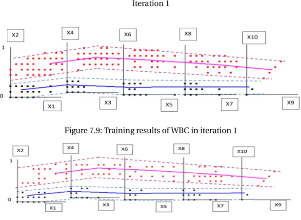
Iteration 1
Figure 7.9: Training results of WBC in iteration 1
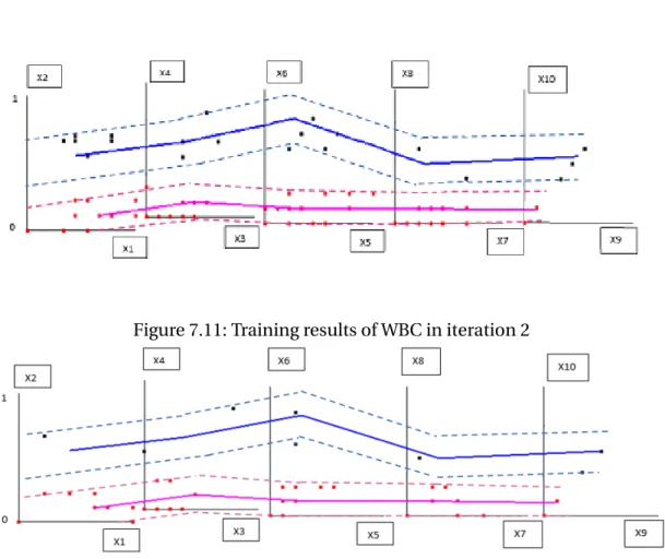
Iteration 2
Figure 7.11: Training results of WBC in iteration 2
Iteration 3
Figure 7.13: Training results of WBC in iteration 3
Figure 7.14: Testing results of WBC in iteration 3
Remaining records
Figure 7.15: Remaining records of class Malignant in training
7.3 L
ETTERR
ECOGNITIOND
ATASET(LR)
In LR dataset there are 20,000 instances and 16 attributes. For the better analysis, we have chosen 2291 instances with 17 attributes including the class to identify the letters AB and C.
The data is split into the ratio 70:30 i.e.,1604 instances in training and 687 instances in testing. There are 789 instances of A, 766 instances of B and 736 instances of C in total.We have combined AB as one class and C as another class. In training, there 1088 instances of AB, 516 instances of C and in Testing there are 467 instances of AB and 220 instances of C. The 2 classes in the data and they are categorized as:
• AB = Class 1, color = red
• C = Class 2, color = black
5 iterations have been performed to cover all the data points. Below tables show the data points considered in each iteration.
Training AB C H11 206 0 H21 0 220 Testing AB C H11 62 0 H21 0 93
Table 7.15: Number of instances in Iteration 1
Training AB C H12 566 0 H22 0 54 Testing AB C H12 246 0 H22 0 51
Table 7.16: Number of instances in Iteration 2
Training AB C H13 144 0 H23 0 63 Testing AB C H13 65 0 H23 0 39
Table 7.17: Number of instances in Iteration 3
Training AB C
H14 130 0
Testing AB C
Training AB C H15 33 0 H25 0 40 Testing AB C H15 29 0 H25 0 8
Table 7.19: Number of instances in Iteration 5
Remaining AB C Training 9 6 Testing 5 2
Table 7.20: Remaining cases in LR(AB,C)
Rules of Iteration:
1. R1 : IfX ∈H11∨H12∨H13∨H14∨H15thenX ∈C l ass1 i.e., AB
2. R2 : IfX ∈H21∨H22∨H23∨H24∨H25thenX ∈C l ass2 i.e., C
• Hj k=
©
X: |Cj ki-Xi|≤Tj ki, i=1,2,3,4,5,6,7,8,9,10,11,12,13,14,15,16
ª
where, j = class, k=iteration, i=coordinate
Centers C11i C12i C13i C14i C15i C21i C22i C23i C24i C25i i=1 0.0 0.5333 0.53 0.6 0.73 0.2667 0.2667 0.2667 0.2667 0.268 i=2 0.0 0.3 0.2 0.26 0.15 0.88 0.78 0.55 0.45 0.68 i=3 0.133 0.4 0.4 0.5 0.53 0.33 0.33 0.33 0.33 0.33 i=4 0.15 0.05 0.10 0.2 0.26 0.5 0.68 0.78 0.6 0.9 i=5 0.4 0.533 0.533 0.4667 0.53 0.133 0.133 0.133 0.2 0.2 i=6 0.15 0.25 0.1 0.2 0.3 0.4 0.55 0.75 0.55 0.65 i=7 0.533 0.4667 0.4667 0.4667 0.4667 0.55 0.2667 0.2667 0.33 0.33 i=8 0.2 0.3 0.25 0.2 0.35 0.45 0.75 0.85 0.65 0.55 i=9 0.4667 0.4667 0.4667 0.4667 0.6 0.4667 0.4667 0.4667 0.4 0.4 i=10 0.3 0.4 0.1 0.15 0.2 0.5 0.6 0.81 0.67 0.4 i=11 0.533 0.466 0.466 0.466 0.466 0.53 0.6 0.6 0.4 0.4 i=12 0.2 0.3 0.05 0.15 0.25 0.86 0.95 0.75 0.65 0.55 i=13 0.4667 0.533 0.533 0.533 0.4667 0.0667 0.0667 0.0667 0.0667 0.0667 i=14 0.05 0.1 0.2 0.15 0.25 0.75 0.85 0.65 0.95 0.5 i=15 0.533 0.6 0.6 0.6 0.466 0.2667 0.2 0.2 0.2 0.2 i=16 0.2 0.25 0.3 0.1 0.15 0.65 0.55 0.75 0.85 0.45
Thresholds T11i T12i T13i T14i T15i T21i T22i T23i T24i T25i i =1 0.5 0.95 1.0 1.0 1.0 0.7 0.6 0.5 0.6 0.3 i=2 0.05 0.05 0.05 0.05 0.05 1.0 1.0 1.0 1.0 1.0 i =3 0.3 0.5 0.6 0.6 0.6 0.6 0.7 0.6 0.75 0.45 i=4 0.05 0.05 0.05 0.05 0.05 1.0 1.0 1.0 1.0 1.0 i =5 1.0 1.0 0.8 0.7 0.7 0.5 0.75 0.55 0.65 0.2 i=6 0.05 0.05 0.05 0.05 0.05 1.0 1.0 1.0 1.0 1.0 i =7 0.3 0.6 0.6 0.6 1.0 0.6 0.8 0.8 0.8 0.1 i =8 0.05 0.05 0.05 0.05 0.05 1.0 1.0 1.0 1.0 1.0 i =9 0.9 0.9 0.95 0.75 1.0 0.8 0.9 0.87 0.7 0.6 i =10 0.05 0.05 0.05 0.05 0.05 1.0 1.0 1.0 1.0 1.0 i=11 0.7 1.0 1.0 0.6 0.65 0.7 0.87 0.75 0.8 0.8 i=12 0.05 0.05 0.05 0.05 0.05 1.0 1.0 1.0 1.0 1.0 i=13 0.5 0.55 0.8 0.8 0.8 0.9 0.7 0.85 0.6 0.75 i=14 0.05 0.05 0.05 0.05 0.05 1.0 1.0 1.0 1.0 1.0 i=15 0.6 0.9 0.8 0.55 0.65 0.75 0.75 0.7 0.65 0.1 i=16 0.05 0.05 0.05 0.05 0.05 1.0 1.0 1.0 1.0 1.0
Table 7.22: Values of thresholds in LR(AB,C)
3. The remaining instances in training phase from the class AB are 9 and from the class C are 6.Hence, the rule can be given as,
R3: If (X=XAB1)∨(X=XAB2)∨(X=XAB3)∨(X=XAB4)∨(X=XAB5)∨(X=XAB6)∨
(X=XAB7)∨(X=XAB8)∨(X=XAB9)⇒Class 1.
R4: If (X=XC1)∨(X=XC2)∨(X=XC3)∨(X=Xc4)∨(X=XC5)∨(X=XC6)⇒Class 2.
4. The remaining instances in testing phase from the class AB are 5 and class C are 2. But, in the testing we cannot know in prior which case is AB or C like we did in training phase. Hence we augment the rule and draw a confusion matrix to show the refused instances in the testing phase which will not be found within the hyper-rectangles and find the accuracy.
AB C Refusal AB 462 0 0
C 0 218 0 Refusal 5 2 0
The results of the iterations are shown in the figures below along with the remaining cases that do not belong to found in the hyper-rectangles in the training and testing
phase.
Iteration 1
Figure 7.17: Training results of LR(AB,C) in iteration 1
Iteration 2
Figure 7.19: Training results of LR(AB,C) in iteration 2
Iteration 3
Figure 7.21: Training results of LR(AB,C) in iteration 3
Iteration 4
Figure 7.23: Training results of LR(AB,C) in iteration 4
Iteration 5
Figure 7.25: Training results of LR(AB,C) in iteration 5
Remaining Instances
Figure 7.27: Remaining instances of class AB in training
Figure 7.28: Remaining instances of class C in training
Figure 7.29: Remaining instances of class AB in testing
Next we conduct an experiment by considering only A, B from the dataset.
The total number of instances are 1555. The data are split into the ratio 70:30 i.e.,1088 instances in training and 467 instances in testing. There are 789 instances of A, 766 instances of B in total. In training, there 552 instances of A, 536 instances of B and in Testing there are 237 instances of A and 230 instances of B. The 2 classes in the data and they are categorized as:
• A = Class 1, color = red
• B = Class 2, color = black
3 iterations have been performed to cover all the data points. Below tables show the data points considered in each iteration.
Training A B H11 206 0 H21 0 200 Testing A B H11 62 0 H21 0 82
Table 7.24: Number of instances in Iteration 1
Training A B H12 200 0 H22 0 145 Testing A B H12 100 0 H22 0 70
Table 7.25: Number of instances in Iteration 2
Training A B H13 140 0 H23 0 185 Testing A B H13 73 0 H23 0 75
Table 7.26: Number of instances in Iteration 3
Remaining A B Training 6 5 Testing 2 3
Rules of Iteration:
1. R1 : IfX ∈H11∨H12∨H13thenX ∈C l ass1 i.e., A
2. R2 : IfX ∈H21∨H22∨H23thenX ∈C l ass2 i.e., B
• Hj k=
©
X: |Cj ki-Xi|≤Tj ki, i=1,2,3,4,5,6,7,8,9,10,11,12,13,14,15,16
ª
where, j = class, k=iteration, i=coordinate
Centers C11i C12i C13i C21i C22i C23i
i=2 0.3 0.05 0.15 0.71 0.82 0.61 i=4 0.35 0.2 0.1 0.75 0.6 0.55 i=6 0.35 0.2 0.1 0.66 0.55 0.45 i=8 0.35 0.2 0.1 0.7 0.85 0.6 i=10 0.35 0.2 0.1 0.7 0.83 0.6 i=12 0.33 0.17 0.06 0.8 0.95 0.7 i=14 0.32 0.17 0.06 0.72 0.96 0.82 i=16 0.35 0.2 0.1 0.7 0.82 0.92 i=1 0.4667 0.4 0.4667 0.26 0.2667 0.2 i=3 0.33 0.31 0.3 0.33 0.3 0.31 i=5 0.533 0.5 0.525 0.2667 0.25 0.26 i=7 0.33 0.3 0.35 0.33 0.3 0.32 i=9 0.46 0.44 0.42 0.4 0.466 0.44 i=11 0.533 0.52 0.51 0.4 0.4667 0.43 i=13 0.4 0.46 0.43 0.1333 0.12 0.13 i=15 0.53 0.5 0.52 0.4 0.4667 0.42
Thresholds T11i T12i T13i T21i T22i T23i i=1 0.5 1.0 1.0 0.6 0.6 0.75 i=2 0.15 1.0 1.0 1.0 1.0 1.0 i=3 0.4 0.6 0.55 0.65 0.55 0.85 i=4 0.15 1.0 1.0 1.0 1.0 0.1 i=5 1.0 1.0 0.75 0.5 0.7 0.66 i=6 0.15 1.0 1.0 1.0 1.0 1.0 i=7 0.8 0.8 0.55 0.6 0.75 0.8 i=8 0.15 1.0 1.0 1.0 1.0 1.0 i=9 0.76 0.93 0.83 0.8 0.88 0.75 i=10 0.15 1.0 1.0 1.0 1.0 1.0 i=11 0.7 0.8 1.0 0.65 0.85 0.7 i=12 0.15 1.0 1.0 1.0 1.0 1.0 i=13 0.5 0.65 0.85 0.45 0.0.8 0.8 i=14 0.15 1.0 1.0 1.0 1.0 1.0 i=15 0.6 0.7 0.85 0.5 0.8 0.65 i=16 0.15 1.0 1.0 1.0 1.0 1.0
Table 7.29: Values of thresholds in LR(A,B)
3. The remaining instances in training phase from the class A are 6 and from the class B are 5.Hence, the rule can be given as,
R3: If (X=XA1)∨(X=XA2)∨(X=XA3)∨(X=XA4)∨(X=XA5)∨(X=XA6)⇒Class 1.
R4: If (X=XB1)∨(X=XB2)∨(X=XB3)∨(X=XB4)∨(X=XB5)⇒Class 2.
4. The remaining instances in testing phase from the class A are 2 and class B are 3. But, in the testing we cannot know in prior which case is A or B like we did in training phase. Hence we augment the rule and draw a confusion matrix to show the refused instances in the testing phase which will not be found within the hyper-rectangles and find the accuracy.
A B Refusal A 235 0 0 B 0 227 0 Refusal 2 3 0
Table 7.30: Confusion Matrix for testing phase in LR(A,B)
The results of the iterations are shown in the figures below along with the remaining cases that do not belong to found in the hyper-rectangles in the training and testing
phase.
Iteration 1
Figure 7.31: Training results of LR(A,B) in iteration 1
Figure 7.32: Testing results of LR(A,B) in iteration 1
Iteration 2
Figure 7.33: Training results of LR(A,B) in iteration 2
Figure 7.34: Testing results of LR(A,B) in iteration 2
Remaining Instances
Figure 7.37: a)Remaining instances of class A in training
Figure 7.38: b)Remaining instances of class B in training
Figure 7.39: a)Remaining instances of class A in testing
Another experiment has been carried out and here we have chosen 1550 instances with 17 attributes including the class to identify the letters T and I.
The data is split into the ratio 70:30 i.e., 1085 instances in training and 465 instances in testing. There are 560 instances of T and 525 instances of I in training, 235
instances of T and 230 instances of I in Testing. There are 2 classes in the data and they are categorized as:
• I = Class 1, color = red
• T = Class 2, color = black
5 iterations have been performed to cover all the data points. Below tables show the data points considered in each iteration.
Training I T H11 104 0 H21 0 178 Testing I T H11 17 0 H21 0 31
Table 7.31: Number of instances in Iteration 1
Training I T H12 154 0 H22 0 102 Testing I T H12 53 0 H22 0 70
Table 7.32: Number of instances in Iteration 2
Training I T H13 127 0 H23 0 91 Testing I T H13 65 0 H23 0 81
Table 7.33: Number of instances in Iteration 3
Training I T H14 99 0 H24 0 159 Testing I T H14 72 0 H24 0 44
Remaining I T Training 7 6 Testing 3 0
Table 7.36: Remaining cases in LR(T,I)
Rules of Iteration:
1. R1 : IfX ∈H11∨H12∨H13∨H14∨H15thenX ∈C l ass1 i.e., I
2. R2 : IfX ∈H21∨H22∨H23∨H24∨H25thenX ∈C l ass2 i.e., T
• Hj k=
©
X: |Cj ki-Xi|≤Tj ki, i=1,2,3,4,5,6,7,8,9,10,11,12,13,14,15,16
ª
where, j = class, k=iteration, i=coordinate
Centers C11i C12i C13i C14i C15i C21i C22i C23i C24i C25i
i=2 0.0 0.06 0.115 0.165 0.222 0.45 0.65 0.55 0.75 0.85 i=4 0.2 0.3 0.1 0.35 0.25 0.55 0.65 0.45 0.78 0.9 i=6 0.1 0.16 0.05 0.2 0.25 0.35 0.55 0.65 0.75 0.45 i=8 0.1 0.15 0.05 0.2 0.3 0.5 0.75 0.85 0.65 0.4 i=10 0.15 0.2 0.1 0.3 0.25 0.5 0.6 0.8 0.7 0.4 i=12 0.05 0.1 0.2 0.15 0.25 0.45 0.55 0.75 0.65 0.35 i=14 0.0 0.1 0.2 0.05 0.15 0.4 0.6 0.7 0.5 0.3 i=16 0.05 0.15 0.2 0.1 0.25 0.65 0.75 0.45 0.55 0.35 i=1 0.0 0.1 0.5 0.53 0.66 0.2 0.2 0.3 0.2 0.067 i=3 0.26 0.267 0.4 0.4 0.53 0.267 0.2667 0.2667 0.2667 0.1 i=5 0.46 0.466 0.45 0.46 0.26 0.133 0.133 0.133 0.13 0.46 i=7 0.5 0.533 0.73 0.72 0.53 0.133 0.133 0.133 0.12 0.13 i=9 0.53 0.533 0.6 0.6 0.5 0.4667 0.4667 0.46 0.45 0.4 i=11 0.53 0.533 0.53 0.5 0.53 0.4667 0.46 0.45 0.4 0.533 i=13 0.53 0.533 0.6 0.6 0.6 0.0 0.067 0.067 0.06 0.533 i=15 0.53 0.533 0.46 0.4 0.45 0.065 0.133 0.13 0.123 0.067
Thresholds T11i T12i T13i T14i T15i T21i T22i T23i T24i T25i i =1 1.0 1.0 1.0 0.8 0.9 0.5 0.5 0.55 0.55 0.3 i=2 0.05 0.05 0.05 0.05 0.05 0.07 1.0 0.05 1.0 0.55 i =3 0.6 0.55 0.55 0.65 0.6 0.55 0.55 0.55 0.55 0.4 i=4 0.05 0.05 0.05 0.05 0.05 0.07 1.0 0.05 1.0 0.55 i =5 0.85 0.85 0.75 0.75 0.07 0.65 0.6 0.45 0.6 0.1 i=6 0.05 0.05 0.05 0.05 0.05 0.07 1.0 0.05 1.0 0.55 i =7 1.0 0.9 1.0 1.0 0.5 1.0 1.0 0.5 1.0 1.0 i =8 0.05 0.05 0.05 0.05 0.05 0.07 1.0 0.05 1.0 0.55 i =9 1.0 1.0 1.0 0.95 0.88 0.75 0.6 0.65 0.75 0.6 i =10 0.05 0.05 0.05 0.05 0.05 0.07 1.0 0.05 1.0 0.55 i=11 0.9 0.95 0.55 0.85 0.65 0.92 0.9 0.85 0.8 0.8 i=12 0.05 0.05 0.05 0.05 0.05 0.07 1.0 0.05 1.0 0.55 i=13 0.88 0.95 0.8 0.95 0.55 0.5 0.45 0.4 0.55 0.1 i=14 0.05 0.05 0.05 0.05 0.05 0.7 1.0 0.05 1.0 0.55 i=15 0.6 0.7 0.85 0.5 0.75 0.55 0.55 0.5 0.6 0.2 i=16 0.05 0.05 0.05 0.05 0.05 0.7 1.0 0.05 1.0 0.55
Table 7.38: Values of thresholds in LR(T,I)
3. The remaining instances in training phase from the class T are 6 and from the class I are 7.Hence, the rule can be given as,
R3: If (X=XI1)∨(X=XI2)∨(X=XI3)∨(X=XI4)∨(X=XI5)∨(X=XI6)∨(X=XI7)⇒
Class 1.
R4: If (X=XT1)∨(X=XT2)∨(X=XT3)∨(X=XT4)∨(X=XT5)∨(X=XT6)⇒Class 2.
4. The remaining instances in testing phase from the class I is 3. But, in the testing we cannot know in prior which case is T or I like we did in training phase. Hence we augment the rule and draw a confusion matrix to show the refused instances in the testing phase which will not be found within the hyper-rectangles and find the accuracy.
I T Refusal I 227 0 0 T 0 235 0 Refusal 3 0 0
The results of the iterations are shown in the figures below along with the remaining cases that do not belong to found in the hyper-rectangles in the training and testing
phase.
Iteration 1
Figure 7.41: Training results of LR(T,I) in iteration 1
Iteration 2
Figure 7.43: Training results of LR(T,I) in iteration 2
Iteration 3
Figure 7.45: Training results of LR(T,I) in iteration 3
Iteration 4
Figure 7.47: Training results of LR(T,I) in iteration 4
Iteration 5
Figure 7.49: Training results of LR(T,I) in iteration 5
Remaining Instances
Figure 7.51: a)Remaining instances of class T in training
Figure 7.52: b)Remaining instances of class I in training
8 SOFTWARE DESCRIPTION
The complete software of this project is presented in a separate folder.
1. The software is developed in C++ using the IDE Visual Studio.
2. The 2-D graphics have been rendered using the API called OpenGL.
3. Data cleaning and mathematical calculations are done using MS-Excel.
9 CONCLUSION
This project displayed the idea of lossless visualization of n-D data as a cognitive enhancer for finding n-D data patters. It incorporates definitions, algorithms and mathematical statements that show how n-D data representations in different general line coordinates simplify the representation of n-D data in 2D for better perceptual and cognitive capacities for discovering visual patterns. The benefits of GLC sub-class of Shifted Paired Coordinates have been appeared on real-world data and demonstrated on visual pattern simplification[9].
The comparison framework has been developed using various datasets like WBC, UKM, and LR performing multiple iterations. The normalized data are split into training and testing.Centers are calculated for every class to visualize the data around them. In each iteration, the data that were used in the iteration has been removed and next iterations are performed on the remaining data. By doing this, we were able to classify well the data among different classes with 100% accuracy and this also reduced occlusion. Hyper-rectangles are built around the centers by considering threshold values. The data that did not found within the bounds of the hyper-rectangles towards the end of the iterations are refused. Hence, the proposed system provided a non-overlapping visual representation of data with the opposite classes.
A medical decision system based on GLC with its subclass SPC has been applied to the task of diagnosing breast cancer. The experiment has been conducted on 70-30% of training-test partition and it is observed that the proposed method yields highest classification accuracy of 99.51% matching the results of literature. The proposed method is applied to LR and it outperforms well in terms of accuracy with 99.35% and a lesser number of iterations compared to the literature. UKM data is treated with SPC to distinguish between the 4 classes of data and we achieved an accuracy of 98.62% with no errors in comparison with the literature.
Other than losslessness, the significantly preferred standpoint of GLC is its
multiplicity, which permits changing them to particular n-D data that is visualized. It is demonstrated that GLC adjustment expands expressiveness of GLC including diminishing occlusion and disentangling visual pattern for the given n-D dataset.
10 REFERENCES
1. Wrolstadt, Jay: Satellite Smashes Terabyte Data Barrier, NewsFactor Sci::Tech, http://sci.newsfactor.com/perl/story/18424.html, June 2002.
2. Wolfgang Muller,Heidrun Schumann,"Visual Data Mining", NORSIGD Info, 2002.
3. Kovalerchuk, B. (2014). Visualization of multidimensional data with collocated paired coordinates and general line coordinates. In Proc. SPIE 9017, visualization and data analysis (p. 90170I).
4. O. L. Mangasarian and W. H. Wolberg: "Cancer diagnosis via linear
programming", SIAM News, Volume 23, Number 5, September 1990, pp 1&18.
5. William H. Wolberg and O.L. Mangasarian: "Multisurface method of pattern separation for medical diagnosis applied to breast cytology",Proceedings of the National Academy of Sciences, U.S.A., Volume 87,December 1990, pp 9193-9196.
6. David J. Slate Odesta Corporation; 1890 Maple Ave; Suite 115; Evanston, IL 60201, David J. Slate ([email protected]) (708) 491-3867, January, 1991
7. H. T. Kahraman, Sagiroglu, S., Colak, I., Developing intuitive knowledge classifier and modeling of users’ domain dependent data in web, Knowledge Based Systems, vol. 37, pp. 283-295, 2013.
8. Kovalerchuk B, Grishin V. Adjustable general line coordinates for visual knowledge discovery in nD data. Information Visualization. 2017 Jul:1473871617715860.
9. Kovalerchuk B. Visual Cognitive Algorithms for High-Dimensional Data and Super-intelligence Challenges. Cognitive Systems Research. 2017 Jun 6.
10. Bertini, E., Tatu, A., & Keim, D. (2011). Quality metrics in highdimensional data visualization: An overview and systematization. IEEE Transactions on Visualization and Computer Graphics, 17(12), 2203-2212.
11. Grishin, V., & Kovalerchuk, B. (2014). Multidimensional collaborative lossless visualization: Experimental study. In Luo (Ed.), CDVE 2014,Seattle, Sept 2014. CDVE 2014, LNCS 8683 (pp. 27-35). Springer.
12. Hibbard, B. (2002). Super-intelligent machines. Kluwer.
13. Dhanabal S, CHANDRAMATHI DS. CLUSTERING OF HIGH DIMENSIONAL DATASET USING K-MAM (MAX-AVG-MIN) METHOD WITH PRINCIPAL COMPONENT ANALYSIS A HYBRID APPROACH. Journal of Theoretical & Applied Information Technology. 2014 Mar 10;61(1).
14. Akay MF. Support vector machines combined with feature selection for breast cancer diagnosis. Expert systems with applications. 2009 Mar 31;36(2):3240-7.
15. Albrecht, A. A., Lappas, G., Vinterbo, S. A., Wong, C. K., & OhnoMachado,L. (2002). Two applications of the LSA machine. In Proceedings of the 9th international conference on neural information processing (pp. 184-189).
16. Pena-Reyes, C. A., & Sipper, M. (1999). A fuzzy-genetic approach to breast cancer diagnosis. Artificial Intelligence in Medicine(17), 131-155
17. Quinlan, J. R. (1996). Improved use of continuous attributes in C4.5. Journal of Artificial Intelligence Research(4), 77-90.
18. Hamiton, H. J., Shan, N., & Cercone, N. (1996). RIAC: A rule induction algorithm based on approximate classification. Technical Report CS 96-06, University of Regina
19. Ster, B., & Dobnikar, A. (1996). Neural networks in medical diagnosis:comparison with other methods. In Proceedings of the
international conference on engineering applications of neural networks (pp. 427-430).
20. Abonyi, J., & Szeifert, F. (2003). Supervised fuzzy clustering for the identification of fuzzy classifiers. Pattern Recognition Letters, 14(24), 2195-2207
21. Polat, K., & Gunes, S. (2007). Breast cancer diagnosis using least square support vector machine. Digital Signal Processing, 17(4), 694-701
22. Adnan Alrabea, A. V. Senthilkumar, Hasan Al-Shalabi, and Ahmad Bader, Enhancing K-Means Algorithm with Initial Cluster Centers Derived from Data Partitioning along the Data Axis with PCA, Journal of Advances in Computer Networks, Vol. 1, No. 2, June 2013
23. Fahim A.M., Salem A.M., Torkey F.A.,Saake,G and Ranadan M.A., â ˘AIJ An Efficient k-means with good initial starting pointsâ ˘A˙I, Georgian Electronic Scientific Journal,Computer Science and Telecommunication vol 2, No19., PP -47 -57 ,2009.
24. Kahraman HT, Sagiroglu S, Colak I. The development of intuitive knowledge classifier and the modeling of domain dependent data. Knowledge-Based Systems. 2013 Jan 31;37:283-95.
25. H.T. Kahraman, Designing and application of web-based adaptive intelligent education system, Ph. D. Thesis, Institute of Science and Technology,
Ankara,2009
28. R. Virgilio, R. Torlone, G.J. Houben, Rule-Based Adaptation of Web
Information Systems, World Wide Web, vol. 10, Springer Science + Business Media, 2007.pp. 443-470.
29. M. Simko, M. Bielikova, User modeling based on emergent domain
semantics,in: 18th International Conference on User Modeling, Adaptation, and Personalization, UMAP 2010, Springer-Verlag, Berlin Heidelberg, 2010, pp.411-414.
30. M. Laguia, J.L. Castro, Local distance-based classification, Knowledge-Based Systems 21 (2008) 692-703