Numerical Experiments with Support Vector Machines

D a l l e M o l l e I n s t i t u t e f o r P e r c e p t u a l A r t i f i c i a l Intelligence • P.O.Box 592 • Martigny • Valais • Switzerland phone +41 – 27 – 721 77 11 fax +41 – 27 – 721 77 12 e-mail secretariat@idiap.ch internet http://www.idiap.ch

August 1999

Numerical Experiments with Support

Vector Machines

Mikhail Kanevski

Nicolas Gilardi

ESE

A

RCH

R

EP

R

ORT

IDI

A

P

IDIAP-RR-99-15

IDIAP

Martigny - Valais - Suisse

1 _{IDIAP – Dalle Molle Institute of Perceptual Artificial Intelligence, CP 592, 1920 Martigny, Switzerland} 2 _{Institute of Mineralogy and Petrology, University of Lausanne, BFSH2, 1015 Lausanne, Switzerland}

Numerical Experiments with Support Vector Machines

M. Kanevski (1), N. Gilardi (1,2),

(1) IDIAP, Case Postale 592, 1920 Martigny, Switzerland. Gilardi@idiap.ch, Kanevski@idiap.ch

(2) Institute of Mineralogy and Petrology, University of Lausanne, Lausanne, Switzerland

Abstract. The report presents a series of numerical experiments concerning application of Support Vector Machines for the two class spatial data classification. The main attention is paid to the variability of the results by changing hyperparameters: bandwidth of the radial basis function kernel and C parameter. Training error, testing error and number of support vectors are plotted against hyperparameters. Number of support vectors is minimal at the optimal solution. Two real case studies are considered: Cd contamination in the Leman Lake, Briansk region radionuclides soil contamination. Structural analysis (variography) is used for the description of the spatial patterns obtained and to monitor the performance of SVM.

1. Introduction ...2

2. Objectives of the experiments ...3

3. Support vector machines. basic formulas...3

SVM classification of linearly separable data...3

SVM classification of nonseparable data ...5

SVM non-linear classification...6

4. Description of the software used...7

5. Case studies...8

Structural analysis. Variography ...9

Leman Lake data ...10

Cs137 soil contamination data ...13

5. Results of the experiments ...16

7. Discussion and Conclusions...29

8. Acknowledgements ...30

9. References ...30

1. INTRODUCTION

The application of the Support Vector Machines for the environmental and pollution spatial data classification has been considered in our previous papers (Kanevski et al 1999, Gilardi and Kanevski 1999). The simplest case of the SVM, namely two class classification, was used. Original continuous data on sediments contamination by Cadmium in the Leman Lake were transformed to the indicator variable. Indicator transform is a non-linear threshold transformation: all data below threshold obtain label “1”, and above threshold – label “0”. This kind of transformation is widely used in geostatistics while performing so-called probabilistic mapping with indicator kriging (Deutsch and Jurnel 1997, Goovaerts 1997). As a result of indicator kriging map of probabilities to be above predefined level/threshold can be established. Comparison between SVM classification and indicator kriging for the selected threshold was carried out in (Kanevski et al 1999). Of course, threshold transformation is a very “hard” transformation. In order to understand the stability of the results (decision surface), several thresholds near the main one were studied as well. It helped to understand the robustness of the results with small changes.

In the research (Kanevski et al 1999) several questions were posed: importance of data pre-processing (transformation of the input space, training/testing data splitting, etc); selection of the optimal hyperparameters (bandwidth of RBF kernel, C parameter); stability of the optimisation algorithms; application of independent criteria for monitoring and control of SVM performance (e.g., variography) and others.

IDIAP-RR-99-07 3

Let us remind, that usually 2 dimensional environmental and pollution data have important multidimensional features like anisotropy, well defined boundary, spatial clustering of data, and they are easy for the visualisation. Moreover, in many practical decision making situations problems can be reduced to 2 dimensional classification/mapping and presentation as a decision-oriented maps with the help of Geographical Information Systems.

The present report deals with numerical experiments using 2D real environmental data. The first case study is an extension of the previous report case study (“Leman”) based on Leman Lake sediments data (Kanevski et al 1999). The second case study (“Briansk”) deals with classification of the radioactively contaminated territories in Russia to be above or below predefined level of contamination. The level 10 Ci/km2 was selected. The latter case study was selected because these data are well understood and have been processed with different approaches and models, including geostatistics, artificial neural networks and wavelets.

Software used for the investigation is described in chapter 4 (see below). Mainly RBF kernels were used. Geostat Office software was used for the data pre-processing, post-processing, structural analysis (variography) and visualisation (Kanevski et al 1999b).

2. OBJECTIVES OF THE EXPERIMENTS

The main part of the study is of methodological nature. Examples are rather straightforward. Posing the problem of spatial classification as a pattern recognition one should be more elaborated. At present the work with a real spatial multivariate categorical data (e.g., soil types) is under development.

In the present research by changing different SVM parameters we have tried to understand consequences both for the learning phase and for the results. It seems that application of the spatial structural analysis (variography) for the monitoring of SVM performance have been used for the first time.

Let us mention the main objectives of the present study: • Check the suitability of SVM for spatial data

• Find indicators of robustness and of efficiency of SVM

• Control the consistency of classification for a series of thresholds • Compare the results of SVM with other methods of spatial statistics

• Influence of the kernel width on the training (TRE) and testing (TEE) error curves and on the number of support vectors (NSVM) in case of spatial data

• Influence of the “C” SVM parameter on the above mentioned characteristics (TRE, TEE, NSVM) • Mapping and classification with different hyper parameters

• Application of the variography to the raw data and to the results of classification to monitor the performance of SVM

3. SUPPORT VECTOR MACHINES. BASIC FORMULAS

There are several good books and tutorials devoted to the theory and applications of Support Vector Machines for solution of basic problems when working with empirical data: classification, regression, probability density function estimation (Vapnik 1995; Vapnik 1998; Cherkassky and Mulier 1998; Haykin 1999; Scholkopf et al 1999, http://svm.first.gmd.de). In the present chapter only basic formulas for the SVM classification are presented for the convenience.

SVM classification of linearly separable data

The following problem will be considered. A set S of points (xi

) is given in R

∈

same class on the same side while maximising the minimum distance between either of the two classes and the hyperplane – maximum margin hyperplane.

Let us remind that data set S is linearly separable if there exist W

∈

R

∈

R such that

W

X

+b

≥

1

if Y

= +1

W

X

+ b

≤

1

if Y

= -1

Very often this inequalities are presented in a more compact way

Y

(W

T

X

+ b)

≥

+1

where index i=1,2,…N.

The pair (W,b) defines a hyperplane of equation

(W

X + b) = 0

Optimal hyperplane with the largest margins between classes is a solution of the following constrained optimization problem (Vapnik 1998, Haykin 1999):

Problem 1(linearly separable data).

Given the training sample {Xi,Yi} find the optimum values of the weight vector W and bias

b

Y

(W

T

X

+ b)

≥

+1

And the weight vector W minimises the cost functions (maximisation of the margins)

F(W)= (½) W

W

The cost function is a convex function of W and the constraints are linear in W.

This constrained optimisation problem can be solved by using Lagrange multipliers. Lagrange function

L(W,b,

α

)=(1/2)W

W -

Σ

α

[Y

(W

X

+b)-1]

where Lagrange multipliers

α

≥

0

The solution of the constrained optimisation problem is determined by the saddle point of the Lagrangian function L(W,b,

α

), which has to be minimised with respect to W and b and to be maximised

α

Application of optimality condition to the Lagrangian function yields

W =

Σ

α

Y

X

Σ

α

Y

=0

Thus, the solution vector W is defined in terms of an expansion that involves the N training data. Note, however, that although this solution is unique by virtue of the convexity of the Lagrangian, the same cannot be said about the Lagrange coefficients.

As far as constrained optimisation problem deals with a convex cost function, it is possible to construct dual optimisation problem. The dual problem has the same optimal value as the primal problem, but with the Lagrange multipliers providing the optimal solution.

IDIAP-RR-99-07 5

Maximise the objective function

Q(

α

)

Σ

α

– (1/2)

Σ

α

α

Y

Y

X

X

Subject to the constraints

Σ

α

Y

=0

α

≥

0 for i=1,2,…N

Note that the dual problem is presented only in terms of the training data. Moreover, the objective

function

Q(

α

)

{

X

X

}

.

After determining optimal Lagrange multipliers

α

calculated as follows:

W=

Σ

α

Y

X

B = 1- W

X

(s)

for Y

= +1

Note that from Kuhn-Tucker conditions it follows that

α

[Y

(W

T

X

+b)-1]=0, for i=1,2,…N

Thus, only

α

the equality sign. The corresponding points Xi , termed Support Vectors, are the points of the set S

closest to the optimal separating hyperplane. In many applications number of support vectors is much less that original data points.

The problem of classifying a new data point X is simply solved by computing

sign(W

X+b)

with the optimal weights and bias.

SVM classification of nonseparable data

In case of linearly nonseparable data it is not possible to construct a separating hyperplane without encountering classification error. The margin of separation between classes is said to be soft if training data points violate the condition of linear separability.

In case of nonseparable data the primal optimisation problem is the following:

Given the training sample {Xi,Yi} find the optimum values of the weight vector W and bias

b

Y

(W

T

X

+ b)

≥

+1-

ξ

for i=1,2,…N

ξ

≥

0

for all i

And the weight vector W and the slack variable

ξ

F(W)= (½) W

W+C

Σ

ξ

where

C

Given the training data maximise the objective function (find the Lagrange multipliers)

Q(

α

)

Σ

α

– (1/2)

Σ

α

α

Y

Y

X

X

Subject to the constraints

Σ

α

Y

=0

0

≤

α

≤

C for i=1,2,…N

Note that neither the slack variables nor their Lagrange multipliers appear in the dual optimisation problem. The parameter C controls the trade-off between complexity of the machine and the number of nonseparable points. It may be viewed as a form of regularisation parameter. The parameter C has to be selected by user. This can be done usually in one of two ways: 1) C is determined experimentally via the standard use of a training (validation) test set, which is a form of re-sampling; 2) It is determined analytically by estimating VC dimension and then by using bounds on the generalisation performance of the machine based on a VC dimension.

SVM non-linear classification

In most practical situations the pattern recognition problems are non-linear and the hypothesis of linear separation in the input space is too restrictive. The basic idea of Support Vector Machines is 1) to map the data into a high dimensional feature space (possibly of infinite dimension) via a non-linear mapping and 2) construction of an optimal hyperplane (application of the linear algorithms described above) for separating features. The first item is in agreement of Cover’s theorem on the separability of patterns which states that input multidimensional space may be transformed into a new feature space where the patterns are linearly separable with high probability, provided: 1) the transformation is non-linear; 2) the dimensionality of the feature space is high enough (Haykin 1999). Cover’s theorem does not discuss the optimality of the separating hyperplane. By using Vapnik’s optimal separating hyperplane VC dimension is minimised and generalisation is achieved. Let us remind that in the linear case the procedure requires only the evaluation of dot products.

Let

{

ϕ

(x)}

space; m – is a dimension of the feature space. Non-linear transformation is defined a priori. In the non-linear case the optimisation problem in the dual form is following:

Given the training data maximise the objective function (find the Lagrange multipliers)

Q(

α

)

Σ

α

– (1/2)

Σ

α

α

Y

Y

K(X

,

X

)

Subject to the constraints

Σ

α

Y

=0

0

≤

α

≤

C for i=1,2,…N

where the kernel

K(X,Y) =

ϕ

(X)

ϕ

(Y) =

Σ

ϕ

(X)

ϕ

(Y)

Thus, we may use inner-product kernel

K(X,Y)

The optimal hyperplane is now defined as

f(x)

Σ

α

Y

K(X,

X

)+b

IDIAP-RR-99-07 7

F(x)=sign[W

K(X,X

)+b]

The requirement on the kernel

K(X,

X

)

Haykin 1999). Three common types of Support Vector Machines are widely used:

1. Polynomial kernel

K(X,

X

)= (X

T

X

+1)

p

where power

p

K(X,

X

)=exp{-||X-X

||

2

/2

σ

}

Where the kernel bandwidth

σ

3. Two-layer perceptron

K(X,

X

)=tanh{

β

X

T

X

+

β

}

Mercer’s conditions are satisfied only for some values of

β

,

β

.

For all three kernels (learning machines), the dimensionality of the feature space is determined by the number of support vectors extracted from the training data by the solution to the constrained optimisation problem. In contrast to RBF neural networks, the number of radial basis functions and their centres are determined automatically by the number of support vectors and their values.

Finally, let us note that Support Vector Machines offer a solution to the design of a learning machine by controlling model complexity independently of dimensionality (Vapnik 1995, 1998):

- Conceptual problem. Dimensionality of the feature (hidden) space is purposely made very large to enable the construction of a decision surface in the form of a hyperplane in that space. For good generalisation performance, the model complexity is controlled by imposing certain constraints on the construction of the separating hyperplane, which result in the extraction of a fraction of the training data as support vectors.

- Computational problem. Numerical optimisation in a high dimensional space suffers from the curse of dimensionality. This computational problem is avoided by using the notion of an inner-product kernel (defined in accordance with Mercer’s conditions) and solving the dual form of the constrained optimisation problem formulated in the input space.

4. DESCRIPTION OF THE SOFTWARE USED

From the previous section it is evident that the most essential part of the SVM implementation consist of quadratic programming module. Recently, several SVM oriented software packages have been especially developed and are available for the scientific study (see home pages at http://svm.first.gmd.de,

http://psichaud.insa-rouen.fr/~scanu). In the present work, Royal Holloway University of London SVM

http://svm.cs.rhbnc.ac.uk ). The RHUL-SV program is a text interface software calculating SVM for a given training file. All the parameters are tuneable, and a large choice of kernel functions is available as well as three different techniques: pattern recognition (two class classification), multiclass classification and regression estimation (epsilon technique).

The main drawback of this software is that it is not possible easily reuse the calculated model and take back the results of classification of an unknown set of data. To avoid this, a PERL script has been generated. It launches the program with the good parameters (some of them decided by the user, while the others hard coded in the script file), extracts the SVM model information from the output file of the RHUL-SV program and then runs the classification of a given data file. Another PERL script launches the RHUL-SV software many times with different parameters in order to create files of error curves indicating the evolution of training error, testing error and the number of support vectors when those parameters are changed.

The RHUL-SV program allows also using three different quadratic optimisers: commercial optimiser MINOS, Alex Smola’s PR_LOQO and Leon Bottou’s optimiser (simply referred as BOTTOU). Only two of those were used in the present numerical experiments: L optimiser (PR_LOQO) and B optimiser (BOTTOU).

All pre-processing and post-processing of data including visualisation have been done with Geostat Office software. Detailed description of Geostat Office along with case study is presented in (Kanevski et al 1999b).

5. CASE STUDIES

Numerical experiments with 2 dimensional spatial data for the two case studies are presented below. The first one is Leman Lake sediments Cd contamination in the year 1988. Let us remind that in (Kanevski et al 1999) this case study was presented as a first trial of using SVM for spatial data classification. Now, we are presenting the comparison between rescaled and not rescaled data, and observe the influence of C parameter in quality of classification (from the testing error point of view). Observation about the correlation between the minimum number of support vectors and the optimal solution area are also shown. Finally, variography is used as a monitoring tool.

The second case study deals with real data on soil contamination of Briansk data by Chernobyl radionuclides. This data set has been widely explored by different spatial statistical models (family of kriging models, probabilistic modelling with indicator kriging, conditional stochastic simulations and cosimulations), artificial neural networks of different architectures (Multilayer perceptrons, Radial Basis Function Neural Networks, General Regression Neural Networks) and hybrid models (ANN+geostatistics). The main results of these studies are described in papers (Kanevski et al. 1996; Kanevski 1999). The main objective of this study was to use SVM to classify indicator at the threshold 10 Ci/km2. An interesting feature of the raw data is spatial non-stationarity and variability at two different scales.

The generic methodology for the analysis, modelling and presentation of spatial data is given in (Kanevski et al. 1999b). From this point of view SVM is only a part of the general flow chart of the procedure. First step usually deals with comprehensive exploratory data analysis. An important part of the study is monitoring network analysis (topology of the distribution of sampling points). Usually, spatial data are collected on a non-homogeneous monitoring network, there are some preferential regions oversampled and some regions are undersampled. This is related to the problem of spatial representativity of the raw data set. In geostatistical analysis different declustering procedures are used to reconstruct global statistics of the data (histogram, mean value, etc.). Another problem deals with dimensional resolution of monitoring network (fractal resolution) – which phenomena can be detected by the monitoring network.

In data driven approaches (artificial neural networks, support vector machines, etc.) data are split into training and testing data sets. The basic technique which is used is related to random splitting. When data are highly clustered, this approach seems to be incorrect. We are using spatial declustering technique in

IDIAP-RR-99-07 9

order extract representative testing data sets. Moreover, variography is used in order to control spatial correlation structures of the data sets. Anyway, this problem should be studied more extensively and carefully.

In accordance with the generic methodology, when using data driven models, variography is applied to the results as well. This helps to monitor and control how much “useful” information (at least described by the first and the second moments of spatial statistics) has been extracted from the raw data. It was shown (Kanevski et al 1996) that this kind of independent (external) control when working with spatial data is useful and efficient.

Structural analysis. Variography

Let us remind some basic notions from the theory of regionalized variables and functions.

Semivariogram (variogram) is the basic tool of the spatial structural analysis variography. Theoretical formula (under the intrinsic hypotheses)

Empirical estimate of the semivariogram

In multivariate case the cross-variogram is used. Theoretical formula for the cross-variogram

Empirical estimate of the cross-variogram

Madogram and rodogram are other measures of spatial correlation (more robust than variogram). Empirical estimate of the madogram

Rodogram. Empirical estimate

Drift is a measure used to characterise global tendencies (trends). Theoretical formula for the drift

D(h)=E{Z(x)-Z(x+h)}

Empirical estimate of the drift is described by the following formula

In the formulas presented above in 2D vector x = (x,y), vector h defines distance and direction between two points in space.

Second order stationarity

R

N

Z

Z

( )

( )

{| ( )

(

)|}

h

h

x

x

h

=

−

+

∑

1

2

{

}

{

(

)

}

γ

γ

M

N

Z

Z

( )

( )

| ( )

(

)|

h

h

x

x

h

=

−

+

∑

1

2

{

}

{

}

[

]

γ

( )

h

=

( )

x

−

(

x

+

h

)

( )

x

−

(

x

+

h

E Z

Z

Z

Z

(

)

(

)

γ

∑

(

)

γ

∑

D

N

Z

Z

( )

( )

{ ( )

(

)}

h

h

x

x

h

=

−

+

∑

1

The random function Z is a second order stationary function if the following conditions are satisfied

E[Z(x)]=m=const for all x

∈

S

E[Z(x+h)Z(x)]-m

=C(h), for all x, x+h

∈

S

In case of second order stationarity there is a relationship between covariance function and semivariogram

γ

(h)= C(0)-C(h) and

γ

(

∞

)=C(0)

γ

(0)= C(

∞

)

Intrinsic hypotheses. (Intrinsic random function). The intrinsic random function Z satisfies the following conditions:

Drift=E[Z(x)- Z(x+h)]=0

Var{Z(x+h)-Z(x)]=2

γ

(h)

In case of second –order stationarity or intrinsic hypotheses variogram depends only on separating vector h and does not depend on the position in space, namely vector x.

Leman Lake data

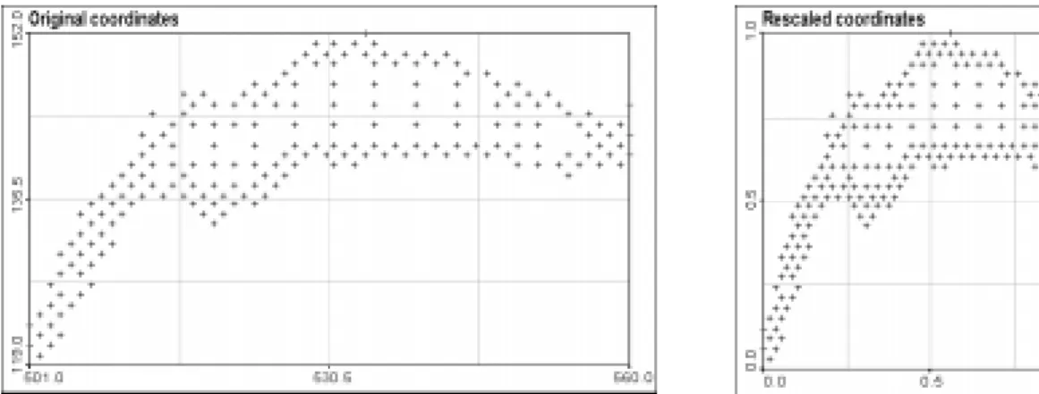
For different reasons very often original data are transformed/projected into some predefined domain. For example, it can be linear transformation of the original input space [Xmin,Xmax][Ymin,Ymax] into [0,1][0,1]. For this reason, we’ve done some experiments in order to see if rescaling of data reduces the efficiency of SVM model.

Fig 1. Presentation of original and rescaled coordinates of data points.

The rescaled data set is simply a projection between zero and one of the X and Y coordinates. The result is a square projection of the Leman Lake. This projection was choosen in order to allow us to understand more easily the meaning of the sigma parameter of the radial basis function kernel.

IDIAP-RR-99-07 11

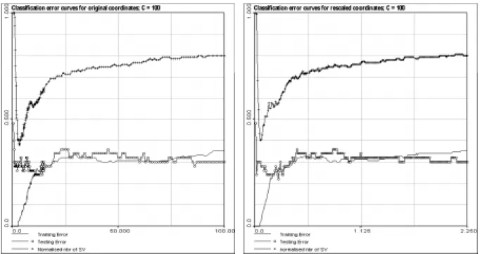
Figure 2. Comparison of error curves for original and rescaled data

In order to compare the influence of rescaling on our data set, we calculated the error curves of each of it. These curves are representing the evolution of training error, testing error and normalised number of support vectors versus RBF kernel parameter. Observing those curves, it appears that they have exactly the same behaviour and nearly the same values. This result allows us to use the rescaled data set for our experiments, as it is easier to interpret.

In the Figure 1 the error curves were calculated for a fixed value of 100 for the C parameter, that upper bound of SV coefficients. But this is a completely arbitrary choice and the question of influence of C value on SV classification efficiency for spatially distributed data is posed.

The comparison of error curves for different values of the C parameter shows that its influence is quite important for our data set classification. As we can see above, behaviour of curves are quite similar. But their values are clearly modified by tuning C. It is interesting to note that for C equal to 100, there is no clear minimum of testing error. In fact there is one, but for this kernel parameter value, training error is more than 15%, so it is very difficult to decide about the quality of this result. For C equal to 104, we have much more clear minimum of testing error (about 16%) corresponding to a quite low training error (about 5%). For C equal to 106, the minimum zone for testing error is more visible, but not so good as it is for C equal to 104.

It is also very interesting to see that the number of support vector has a very precise behaviour. And also, we can easily remark that its minimum area is corresponding to the optimality area, in term of both training and testing errors. While the testing error has a very big variability, the number of support vector seems to be more robust. So, it can be considered as a good indicator of optimality region.

Now that we have found parameters giving an optimal couple for testing error and training error, we can create and use a model based on those parameters, and then, check visually the quality of the results.

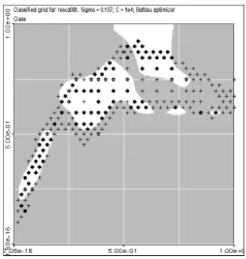
Fig 4. “Optimal” classification of Cd 0.8 level of contamination of Leman Lake sediments

The above picture represents the result of classification for a regular grid with the optimal model defined before (sigma equal to 0.137 and C equal to 10^4). The complete (training and testing) original data set is pictured also.

The results are in a very good accordance with the classified data, and the observation of these shapes gives us a better idea of the efficiency of the method as the fitting area are neither “too much simple” nor “too much complicated”. Of course, this is not a mathematical criterion, but it is interesting as it takes into account not only mean criteria (mean error, variance, etc…) but also spatial repartition. Its drawback is to be quite subjective, but shape analysis techniques can be applied to find more “robust” decision criteria.

IDIAP-RR-99-07 13

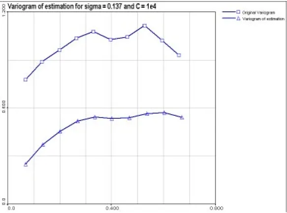
Figure 5. Omnidirectional variograms of the original data set and optimal estimation

Presented in Figure 5, the comparison between original data variogram (with squares) and “optimal” estimation (with triangles) shows many interesting things. First, as the two variograms are represented at the same scale, it is obvious that the estimation variogram has less nugget effect (local uncertainty) than the original one. This is a direct effect of modelling. Second, the general shapes appear to be quite similar, but the model is softer than the original. In fact, if the model is able to reproduce the short range correlation between data points, the large scale effects are not forgotten but not very efficiently modelled.

By the way, the Leman Lake case study is a quite difficult one, and not enough information on previous analysis are available.

Cs137 soil contamination data

Data have been described in detail in several publications (Kanevski et. al, 1996). The original data set containing 665 measurements of Cs137 was spit into training and testing data sets. Method of spatial declustering technique were used to have representative training data set. In the present case study 200 points were used for training and 465 points for validation. Actually data were split into different proportions as well and with different techniques, including random selection. In the present paper only results of numerical experiments with 200 training and 465 testing points are reported. Some effects of data splitting on the results is presented in the previous section with the artificial data set. The contamination level of 10 Ci/sq.km was selected for the analysis. Input space (X,Y) from [Xmin,Xmax]x[Ymin,Ymax] region was transformed linearly to the [0,1]x[0,1] region.

This data set has been studied a lot not only from practical point of view but also from scientific point of view: data are highly variable at several scales (the consequence of atmospheric processes and deposition), data are spatially non-stationary, there is well defined anisotropy in spatial correlation

(described by variograms and other spatial correlation functions). It should be noted, that hybrid models (ANN + geostatistics) were developed and applied for this data set.

Because in the present work we are dealing with the simplest spatial problem – problem of spatial classification, original data were transformed into indicators at the threshold 10 Ci/sq.km. Thus, we are posing problem as an environmental pattern recognition problem. The stability (robustness) of the solution (stability of the solution with small changes of threshold) will be studied separately.

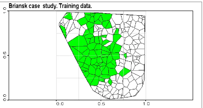
Figure 6. Briansk indicator data. Visualisation of training data set with Voronoi polygons. Variogram rose of the raw indicators was calculated using Geostat Office software. There is an geometric anisotropic spatial correlation structure: in different directions ranges of correlation differ (Goovaerts 1997). These anisotropic variograms can be modelled and used in indicator kriging. Indicator kriging give a probability map of being above threshold (Kanevski et al 1999). SVM was compared with indicator kriging in the previous IDIAP research report. It was shown good agreement between models.

Another important task with variogram interpretation deals with variogram behaviour near the origin (so-called nugget effect). It gives an indication how much of information is spatially structured and how much is related to small scale variations or to noise (e.g., measurement errors). In the worst case (pure nugget effect) data are not spatially correlated that means neighbour points are not relevant each other.

Basically, the main task of any learning from data algorithm is to extract all “useful” information. If there is no spatial structure, at least, described by spatial correlation, data can be described as a noise.

IDIAP-RR-99-07 15

Figure 7. Briansk data. Variogram rose of raw indicators.

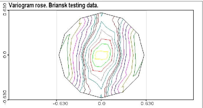
Figure 9. Variogram rose of testing indicator data.

Figure 10. Directional variograms of the training data.

5. RESULTS OF THE EXPERIMENTS

Below in Figures 11-30 there is a gallery of the SVM training error curves and classification results with LOQO and BOTTOU optimisers. Results are discussed at the end of the section.

IDIAP-RR-99-07 17

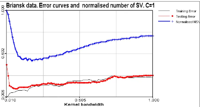
Figure 11. Error curves and normalised number of support vectors. C=1.

Figure 13. Error curves and normalised number of support vectors. C= 106

Figure 14 . Briansk data. Normalised number of support vectors (Nsvm / Ndata) versus kernel bandwidth at different C values.

IDIAP-RR-99-07 19

Figure 15. Training error surface. LOQO optimiser.

Figure 17. Briansk data. Number of support vectors versus kernel bandwidth and C. LOQO optimiser.

Figure 18. Briansk indicator data classification. LOQO optimiser. Kernel bandwidth sigma=0.01. C=100, number of support vectors = 200 = all training data (indicated as “+”). Validation data are indicated as well.

IDIAP-RR-99-07 21

Figure 19. Briansk indicator data classification. LOQO optimiser. Kernel bandwidth sigma=0.04. C=100, number of support vectors = 134 (indicated as “+”). Validation data are indicated as well.

Figure 20. Briansk indicator data classification. LOQO optimiser. Kernel bandwidth sigma=0.1. C=100, number of support vectors = 50 (indicated as “+”). Validation data are indicated as well.

Figure 21. Briansk indicator data classification. LOQO optimiser. Kernel bandwidth sigma = 0.5. C=100, number of support vectors = 70 (indicated as “+”). Validation data are indicated as well.

Figure 22. Briansk indicator data classification. LOQO optimiser. Kernel bandwidth sigma=1.0. C=100, number of support vectors = 86 (indicated as “+”). Validation data are indicated as well.

IDIAP-RR-99-07 23

Figure 23. Briansk indicator data classification. (LOQO) L optimiser. Kernel bandwidth sigma=1.0. C=1e6, number of support vectors = all training data (indicated as “+”). Validation data are indicated as well. Compare with the results of Bottou optimiser for the same hyperparameters.

Figure 24. Briansk indicator data classification. Bottou optimiser. Optimal kernel bandwidth. C=1, number of support vectors = 93 (indicated as “+”). Validation data are indicated as well.

Figure 25. Briansk indicator data classification. Bottou optimiser. Optimal kernel bandwidth. C=100, number of support vectors = 50 (indicated as “+”). Validation data are indicated as well.

Figure 26. Briansk indicator data classification. Bottou optimiser. Optimal kernel bandwidth. C=1e6, number of support vectors = 41 (indicated as “+”). Validation data are indicated as well.

IDIAP-RR-99-07 25

Figure 27. Briansk indicator data classification. Bottou optimiser. Kernel bandwidth sigma=1.0 (ovesmoothing). C=100, number of support vectors = 88 (indicated as “+”). Validation data are indicated as well. Compare these results with the same hyperparameters but with L (LOQO) optimiser.

Figure 28. Briansk indicator data classification. Bottou optimiser. Kernel bandwidth sigma=1.0 (ovesmoothing). C=106, number of support vectors = 58 (indicated as “+”). Validation data are indicated as well. Compare the results with the same hyperparameters but with LOQO optimiser.

Figure 29. Briansk data. Bottou optimiser. Number of support vectors versus kernel bandwidth.

Figure 30. Briansk data. Error curves at C=100. B optimiser.

In the figure describing the number of support vectors versus kernel bandwidth the presence of the minimum on the curves is evident. Moreover, this minimum is located in the region of optimal solution selected form testing error curves. This is very important, because near the optimal solution the number of important data points representing support vectors are minimal which proves the efficiency of SVM.

Vapnik gave a bound on the actual risk of support vector machines (the leave-one-out bound, or cross-validation bound):

IDIAP-RR-99-07 27

E[P(error)]

≤

E{Number of support vectors}/{Number of training samples}

Where P(error) is the actual risk for a machine trained on (N-1) examples, E[P(error)] is the expectation of the actual risk over all choices of training set of size (N-1), and E{Number of support vectors} is the expectation of the number of support vectors over all choices of training sets of size N.

In (Burges 1998) the influence of kernel bandwidth on error curves and number of support vectors have been studied. NIST digit data set was used as a case study. It was observed, that cross-validation bound, although tighter than VC bound, did not seem to be predictive, since it had no minimum for the values of sigma studied.

In fact, it seems reasonable, that number of support vectors under the fixed C value has to increase with increasing of sigma. Kernels are more and more simple with increasing sigma and more and more support vectors are needed to describe even simple functions. Of course, sigma value has to be compared with characteristic ranges of the problem under study or with the scale of the region. For the large sigma the kernel can be represented as

K(X,

X

)=exp{-||X-X

||

2

/2

σ

}=1 - ||X-X

||

2

/2

σ

at ||X-X

||/2

σ

<<1

Let us note that in the present study minimum near the optimal from the testing point of view region was found in wide range of “C” parameter values. Moreover, sometimes it was difficult, if possible to find minimum on a testing error curves, while it was clearly detected on the number of support vector curves. It seems that this problem has to be studied more both from analytical and numerical points of view. In the figure presented for the B optimiser and C=100 minimum for the two curves coincides. In this case it seems reasonable to look at minimum number of the support vectors and to take this sigma value as the optimal (even without splitting of data into training and testing sets). With minimum number of support vectors developed model is more stable and has better generalisation capabilities.

In order to understand spatial correlation structures of the results obtained variography was used. We have calculated omnidirectional variograms for the results obtained with different C and sigma parameters. In general, good results (almost the same for L optimiser and B optimiser) were obtained at C=100. That’s why only these results are presented for the qualitative and quantitative behaviour of the variograms in the figure below.

Figure 31. A selection of omnidirectional variograms calculated for the raw data and results. C=100. L optimiser.

Omnidirectional variograms of the results (Figure 31) give indication of their relevance in comparison with original raw data (at least, in terms of spatial correlations). Of course, variogram of the overfitted data represents almost pure nugget effect (very small scale variations) which is near the original nugget effect presented in raw variogram. Variogram of the optimal classification almost fit raw variogram. This was an “unexpected” result of the SVM classification. Increasing smoothing by enlarging kernel bandwidth results in smoother variogram behaviour. Thus, variograms can be used as a good qualitative and even quantitative tool. It seems that these kind of numerical experiments are promising and should be carried out for different case studies having different multiscale and anisotropic structures.

IDIAP-RR-99-07 29

Figure 32. Variogram “surface”. Y-axis represent kernel bandwidth of SVM. Cross-sections along X-axis determines variograms. “C” parameter was fixed: C=100.

7. DISCUSSION AND CONCLUSIONS

The present study has dealt with the simplest problem of two-class classification with the Support Vector Machines. By performing the present study we have postponed jump to more interesting and important problems like multiclass classification of environmental spatial data (e.g., soil types), spatial regression problems and local probability density function modelling (probabilistic mapping with SVM). The main reason was to understand more about SVM developments and their applicability to spatial data at this level. Many of the problems have still to be better understood and solved. Nevertheless, we can conclude, that SVM are a powerful tools for the spatial data classification. Robustness of the SVM with threshold fluctuations is under development.

Near the optimal solution the number of support vectors is minimal (which is a nice and an important property of the SVM).

Spatial structural analysis is an independent tool for the monitoring and quality control of the SVM classification. In case of classification variography can be considered as a qualitative tool rather than quantitative instrument (selection of the “best”/optimal solution by using variogram is rather difficult). Nevertheless, variogram analysis easily indicates overfitting and oversmoothing regions.

Stability of the SVM algorithms should be studied more, especially in the regions of oversmoothing and with large values of “C” parameter. It seems that some optimisers may have problems in this region of hyper parameters.

Another independent tools developed in mathematical morphology (shape analysis) may be adapted and used for the monitoring and control of SVM classification.

Real multiclass classification environmental problem is a nearest interesting future of the study. Future studies of the spatial regression problems are the following:

Comparison of the spatial regression with SVR and comprehensive comparisons with geostatistical models.

Spatial nonstationarity problems can be solved with hybrid/mixed models = Support Vector Regressors + geostatistics, when large scale non-linear trends can be modelled by small fraction of the support vectors and local variability can be reconstructed by, e.g. geostatistical predictors or stochastic simulators.

Presented above results show that in the region of overfitting and near optimal solution different optimisers give almost the same results even for the wide range of “C” parameter. In the region of oversmoothing results differs considerably especially for large “C” values. Basically, this region with large possible solutions is numerically unstable, and care should be taken using in this region with any optimiser. In fact, practically this region is not interesting.

8. ACKNOWLEDGEMENTS

The work was supported in part by Swiss National Research Foundation (Cartann project: FN 2100-054115.98) and by European INTAS grants 96-1957, 98-31726. The work was carried out during M. Kanevski’s stay at IDIAP and INSA (Rouen, France) as an invited Professor. The authors thank to Geostat Office group (IBRAE, Moscow) for the access to the Geostat Office software and RHUL SVM group for the possibility to use their software for the present scientific research. Special thanks to Dr. E. Mayoraz, Prof. M. Maignan and Prof. S. Canu for many valuable discussions on the theory and implementations.

9. REFERENCES

Boser B.E., I.M. Guyon, and V. Vapnik. A training algorithm for optimal margin classifiers, In Fifth

Annual Workshop on Computational Learning Theory, Pittsburgh, 1992. ACM.

Burges C.J.C. A tutorial on Support Vector Machines for patterns recognition. To appear in Data Mining

and Knowledge Discovery. 1998.

Cortes C. and V. Vapnik. Support vector networks. Machine Learning, 20: 273–297, 1995. Cherkassky V and F. Mulier. Learning from data. John Wiley & Sons, Inc. N.Y. 441 p. 1998.

Cristianini N., Campbell C., J. Shawe-Taylor NeuroCOLT2 Technical Report Series, NC2-TR-1998-017. 12 p. 1998

Deutsch C.V. and A.G. Journel. GSLIB. Geostatistical Software Library and User’s Guide. Oxford University Press, New York, 1997.

N. Gilardi, M. Kanevski, M. Maignan and E. Mayoraz. Environmental and Pollution Spatial Data

Classification with Support Vector Machines and Geostatistics. Greece, ACAI’99. July 1999, pp. 43-51.

Goovaerts P.. Geostatistics for Natural Resources Evaluation. Oxford University Press, New York, 1997. Haykin S. Neural Networks. A Comprehensive Foundation. Second edition. Prentice-Hall, Inc. New Jersey, pp. 318-350, 1999.

Kanevski M., Arutyunyan R., Bolshov L., Demyanov V., Maignan M. Artificial neural networks and spatial estimations of Chernobyl fallout. Geoinformatics. Vol.7, No.1-2, pp.5-11, 1996.

Kanevski M., N. Gilardi, M. Maignan, E. Mayoraz. Environmental Spatial Data Classification with

Support Vector Machines. IDIAP Research Report. IDIAP-RR-99-07, 24 p., 1999.

Kanevski M., V. Demyanov, S. Chernov, E. Savelieva, A. Serov, V. Timonin, M. Maignan. Geostat Office for environmental and pollution data analysis. Mathematische Geologie, Dresden, April 1999b. Kanevski M. Spatial Predictions of Soil Contamination Using General Regression Neural Networks. Int. J. on Systems Research and Information Systems, Volume 8, number 4. Special Issue: Spatial Data:

IDIAP-RR-99-07 31

Neural nets/Statistics. Guest Editors Dr. Patrick Wong and Dr. Tom Gedeon.Gordon and Breach Science Publishers, pp. 241-256. 1999.

Smola A.J. and B. Schölkopf. A tutorial on Support Vector Regression. NeuroCOLT2 Technical Report

Series, NC2-TR-1998-030. October, 1998.

Vapnik V.. The Nature of Statistical Learning Theory. Springer-Verlag, New York, 1995.

Weston J., A. Gammerman, M. Stitson, V. Vapnik, V. Vovk, C. Watkins. Density Estimation using Support Vector Machines. Technical Report, Csd-TR-97-23. February 1998.