Combining Sequential and Aggregated Data for Churn Prediction in
Casual Freemium Games
Jeppe Kristensen and Paolo Burelli
Abstract— In freemium games, the revenue from a player comes from the in-app purchases made and the advertisement to which that player is exposed. The longer a player is playing the game, the higher will be the chances that he or she will generate a revenue within the game. Within this scenario, it is extremely important to be able to detect promptly when a player is about to quit playing (churn) in order to react and attempt to retain the player within the game, thus prolonging his or her game lifetime. In this paper we investigate how to improve the current state-of-the-art in churn prediction by combining sequential and aggregate data using different neural network architectures. The results of the comparative analysis show that the combination of the two data types grants an improvement in the prediction accuracy over predictors based on either purely sequential or purely aggregated data.
I. INTRODUCTION
Games distributed using the freemium business model are freely downloadable and playable. The main revenue for the games comes from virtual goods that can be purchased by players. Furthermore, many games include some form of advertisement (e.g. banners) that serve as a supplementary revenue stream.
In the freemium industry, similarly to other service indus-tries such as telecommunications, the revenue that a player can generate is proportional to the duration of the relationship between the player and the game/service. Therefore, increas-ing player retention (i.e. the duration of the period before a player quits) is commonly considered an effective strategy for increasing lifetime value [25].
This can be achieved in many ways, for example by producing more content for players in end-of-content situ-ations or by adjusting problematic sections in the game that have shown to lead players to quit. Another possible way, as shown by Milosevic[20], is to identify the players that are likely about to stop to playing (i.e. churn) and target them with a personalised re-engagement initiative before they abandon the game.
This is challenging especially in non-contractual services such as freemium games. For contractual services, such as telephone subscriptions or newsletters, the churn event is well defined, and corresponds to the moment when the contract expires or is cancelled. However, for non-contractual services, such as games or retail, there is not an explicit event that signals that a user stops using the service.
The most common way, as described by Hadiji et al. [8], is to define the churn time as the time of the last event The authors are with the are with the IT University of Copenhagen and with Tactile Games ApS. (e-mail: jeppek@tactile.dk; pabu@itu.dk). A special thanks goes to Thomas Bjarke Heiberg-I¨urgensen and Rune Viuff Petersen for their MSc thesis work.
produced by a player before being inactive for a certain period of time. The duration of the inactivity may be very different depending on the context: for example, if a player does not return to a freemium game after one week it is much more likely that he/she has churned compared to not returning to a clothing retail shop after a week. Formalising churn is therefore industry and time scale dependent and has to take into account the applicability to the business.
Regardless of the churn definition, churn prediction is currently actively researched in number of different in-dustries including telecommunication providers [24], [9], insurance companies [32], pharmaceutical companies [29] and games [16].
Within games, a number of techniques have been em-ployed for churn prediction ranging from a number of super-vised learning models based on aggregated player data [8], [27] to more recent works that try to leverage the dynamics for the player behaviour by using temporal data [15].
The main reason to use this kind of data is that the changes in the user behaviour leading up to the churn event are potentially more predictive than aggregated data. Such an assumption is supported by a number of other recent studies on churn prediction in other industries [7], [18], [30].
However, since these temporal based methods focus on the dynamics of the player behaviour in a limited time window, they are unable to capture the baseline behavioural patterns of the players and assume that a specific sequence of events determines churn independently of the player’s history and context.
Inspired by the work of Leontieva and Kuzovkin [17] on combining static and dynamic features for classification, in this paper we investigate how both sequential and historic aggregated data about the player behaviour can be used in churn prediction models. We evaluate a number of different architectures than can be used to combine the two types of data and we showcase the results in a comparative analysis based on data from a commercial free-to-play game.
II. RELATED WORK
While the concept of customer churn has been used in research for many years, the first examples of models for churn prediction start to be published in the late nineties and the early two thousands [19], [21]. In their works, Masand et al. and Mozer et al. employ artificial neural networks (with slightly different topologies and feature selection methods) to predict whether a customer will cancel their telephone sub-scription or not. Other methods, such as decision trees [14] **FIND OTHER REF**, support vector machines (SVM)
[31] and logistic regressions, have also been used extensively for churn prediction [13], [9], [6], with many variations detailed in [28].
All of the aforementioned methods for churn prediction attempt to assess the likelihood of a customer to churn based on their past behaviour expressed as a static summary of their state. These models assume that conditions leading to a churn event are based only on a given state of the customer rather than the way customer reached that given state. This means that, for instance, two players with the same average number of hour played per day would be classified in the same way event if one of the two is playing increasingly more while the other is progressively stopping.
To capture this type of differences, the inputs to the model need to incorporate a temporal dimension. This dimension can be either approximated (e.g. incorporating trend and standard deviation to the aggregated measure) or the model can process the inputs as time series. Castro and Tsuzuki [4], for instance, analyse a number of methods to approximate the dynamics of the customer behaviour using different forms of frequency based representations.
If a feature can be arranged into time-sequential bins (e.g. hourly score, daily time played, monthly minutes on call), a more complete representation of the dynamic behaviour can be expressed in the form of a multi-variate time series, in which each sample of customer behaviour is described as a matrix withntrows andnfcolumns, wherentis the number
of time steps/length of time-series andnf is the number of
features.
Prashanth et al. [24] present two different ways of pro-cessing time series using machine learning models. In their compararive study, in one of the case, they employ a long short-term memory (LSTM) [11] recurrent neural network using the data directly as time series.. In the other case they flatten the multivariate time-series matrix into a single vector with lengthnt·nf. By flattening the time-series, additional
static features such as days since last usage and age can be appended to the vector. This vector is then used as input to non-sequential models such as a random forest classifier (RF) and a deep neural network.
A similar approach is used [14] where the static features (e.g. user age) are repeated for each month for the sequential models. While the performance of the different models is comparable, in both papers the RF outperformed the LSTM approach in terms of area under the curve (AUC). Another architecture that allows using sequential data is Hidden Markov Models which is used in [26].
One issue with framing churn prediction as a binary classification problem is that we do not know if/when a customer churns in the future. Because this information is hidden in the future the data is said to be right-censored. So, instead of framing the churn prediction as a binary classification problem methods such as survival analysis attempt to estimate the time to the next event of interest, for instance the return of the customer or cancellation of subscription.
Survival analysis is extensively used in engineering and
economics, and popular methods include Cox Proportional Hazards Model [5] and Weibull Time To Event model [1]. Both methods have been also applied to churn prediction alone and in combination with other classifiers [12], [23], [18], [7].
A. Churn prediction in games
As well as in the other industries, within the games context, the two main approaches for churn prediction consist in either considering churn a classification problem or a survival analysis problem.
In [23], Perianez et al. interpret churn prediction as a survival analysis problem and focus on predicting churn for high-value players using a survival ensemble model. One of the first example of churn prediction as classification instead is the 2014 article by Hadiji et al. [8].
In this work, the authors describe two different forms of churn classification problems, in which the algorithm is either trained to detect whether the player is currently churned (P1) or whether the player will churn in a given future period of time (P2). Furthermore, they compare a number of classifiers based on aggregated gameplay statistics on both tasks on datasets from five different games, showing decision trees to be the most promising classifier.
In the same year, Runge et al. [27] present an article investigating how to predict churn for high value players in casual social games. In this paper, high value player are defined as the top 10% revenue-generating players, the churn definition is similar to the one labelled as P1 by Hadiji et al. [8], and the period of inactivity used to determine churn is 14 days.
A set of classifiers similar to [8] – with the addition of support vector machines – is evaluated on the dataset from two commercial games. For the feed forward neural network and logistic regression models it was found that 14 days of data prior to the churn event leads to the highest AUC.
Furthermore, to include a temporal component in the model, sequences of the daily number of logins are processed through a Hidden Markov Model (HMM). The output of the HMM is then used as an extra input feature. The authors, however, find the the inclusion of the temporal data using HMM degrades the results and hypothesise this might be due to data over-fitting.
A Hidden Markov Model is also used by Tamassia et al. [30] in comparison with other supervised learning clas-sifiers based on aggregated data. The comparative study, conducted on data from the online game Destiny1, shows
an advantage in processing the player behaviour as temporal data.
Kim et al [15] also investigate the predictive power of sequential data by evaluating an Lon-Short Term Memory (LSTM) Neural Network model in predicting churn for new players. In this work, the input data to the LSTM corresponds to a single time series containing the player score recorded every 10 minutes over 5 days; churn is defined as having no activity for 10 days after the first 5 days of observation.
The results show that the LSTM model is able to outper-form both a one-dimensional convolutional neural network on the same time series data and traditional learning models (RF, Gradient boosting, logistic regression) in terms of AUC. A similar result is achieved also by the LSTM based model by YOKOZUNADATA in the churn prediction competition article by Lee at al. [16].
Outside of the context of churn prediction in games, Leontjeva and Kuzovkin [17] show in their article that a hybrid LSTM network combining aggregated and time-series data is capable of better churn prediction than methods using only one of the two data types or classical ensemble methods. These results combined with the aforementioned results by the YOKOZUNADATA LSTM based model suggest that there is potential for hybrid LSTM networks to leverage the combination of aggregated an time-series data. For this reason, in this article we present a comparative study of multiple hybrid architectures of LSTM to evaluate the best solution of the churn prediction problem.
III. METHODS
In this study, we compare a number of different hy-brid LSTM architectures that combine time-series data with aggregated data against commonly employed LSTM neu-ral network and random forest algorithms. In this section, we describe all the architectures, the algorithms and the settings employed, while in the next section, we describe the evaluation procedure. However, before describing the algotihms, it is first necessary to define what definition of churn will be used to label the data foe the algorithms training and evaluation. This choice motivates what kind of data is relevant and can be used and that, in turn, will also determine what kind of architectures can be tested.
A. Churn definition
In freemium games the relationship between a player and the game is typically non-contractual in nature because the user can stop playing the game without any notice. In this situation there is not clear churn event, like a customer cancelling a subscription. For this reason, different research works have slightly different definition of churn; however, they all agree that a player can be considered churned if inactive for a long enough period of time [16].
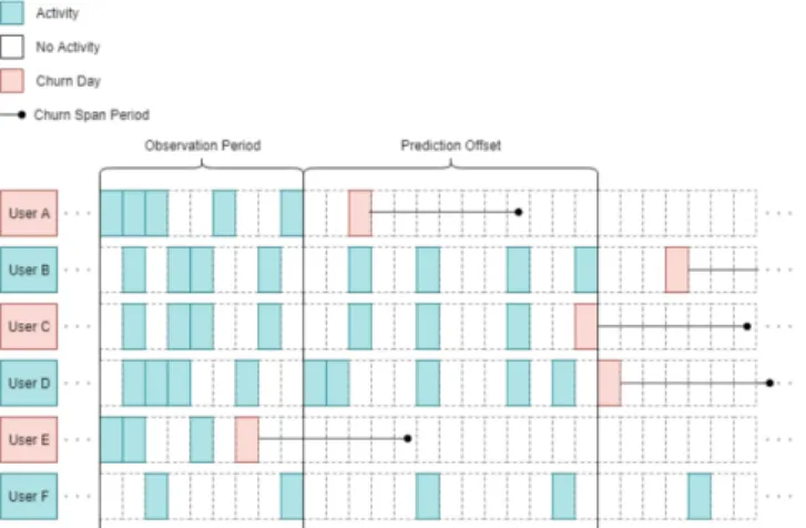
In this work, we define a churn event as the last event generated by a player before a period of inactivity. The churn prediction task, similarily to theP2definition in [8], consists in predicting whether churn event will accurr in the next prediction period (e.g. the week following the prediction). Figure 1 show a number of examples of patterns of player activity and explains whether the players are considered churned or not according to our definition.
A second aspect of the churn classification task that we need to specify is at which players is this model targeted. Kim et al. [15] describe a model aimed at predicting churn for new players, while Runge et al. [27] and Perianez et al [23] focus on high-value players.
Fig. 1. Depiction of the churn definition used to label the data. The predictions are made the day after the last day of the observation period/first day of the prediction offset. In this example user A, C and E are labelled as churners because their churn dates – i.e. the last active day before a period of inactivity (churn span period) – happen before the end of the prediction window. Even though user B and D have a churn date, they are labelled as non-churners because it happens after the prediction window. This is not a problem since their churn will be detected at a later prediction when it is appropiate to reengage them. User F is continuously active and does therefore not churn either. Image curtesy of [10].
The churn definitions in this paper will follow the defini-tions in the thesis of Heiberg-I¨urgensen and Petersen [10]. Here a churn date is defined for each player as a date followed by a given period of inactivity. If this churn date happens in the observation period or in a prediction offset window, the player is labelled as having churned. See Fig. 1 for a graphical overview.
Choosing an appropriate inactivity duration is a trade-off between finding actual churners versus players just taking a break. Even though playing sessions in mobile casual games are generally not very long and ——WORD FOR NON-COMMITTAL——, and are thus somewhat independent of external factors, there are weekly playing patterns. Because of the weekly variations, a minimum requirement for inac-tivity duration should be at least one week, preferably two to ensure the absence is significant. The maximum duration is not clear cut and can be chosen from a business perspective. If the cost of reengaging churning players is low, a short inactivity period can be chosen, and vice-versa. In this paper the churn span period, i.e. duration of inactivity before being labelled as churner, is set to be 30 days.
In order to choose a reasonable observation period, a few aspects have to be considered. While full sequences of each player’s behaviour can be used, it is typically the behaviour leading up to churn event that we need to capture (e.g. getting stuck on a level). Additionally, given the fact that our churn definition also allows the churn to happen inside the observation period, a too long observation period will not tell us whether the player is about to churn soon or has already churned. It is therefore more viable to choose a limited observation period, which speeds up training of the sequential models. A similar argument can be made as for the churn period – a minimum of two weeks should be
used to capture weekly variations. An observation period of 14 days is therefore used.
Lastly, in order to create actionable predictions, a sliding prediction offset window from a given cut-off date (end of observation period) is used in which the churn can happen, similar to theP2definition in [8]. This allows for preemptive actions to be taken when a player about to churn, instead of when he/she has already churned. The length of the prediction offset window is 7 days.
B. Models
In order to test whether adding static player data to the models improves the predictions, three models which only use the sequential data are used as a baseline.
Baseline models: The first two baseline models are a random forest classifier and a feed forward neural network. Because these models can not handle sequential data, the sequences are flattened into a single vector of length10·14 = 140. The last baseline model consists of an LSTM, which can handle sequential data.
The output dimension of the LSTM is set to 16. Heuris-tically using a larger dimension did not improve the predic-tions and typically cause the model to overfit.
For creating and training the neural network models Keras2is used. The random forest model and cross validation
split from scikit-learn3 are also used.
Stacked LSTM: In [2] a stacked LSTM is used for churn prediction because such an architecture may extract features of different timescales [22].
In this paper four LSTMs with 32 units each are stacked upon each in a uni-directional way. The first three cells return sequences that are used as input for the subsequent cell, while the last layer returns a single activation which is then fed into the output layer.
LSTM Activation + Aux:
LSTM Predict + Dense Aux: [17] LSTM Hidden State:
Static in LSTM:
IV. EVALUATION
The data used in this paper is from a casual mobile pop shooter game (see Fig. 2) and contains data samples from 2017-06-01 to 2019-03-04. However, because we can not know whrther a player has churned until the inactivity period and prediction offset period have passed, the latest data is at least 30 + 7 = 37days before the upper-bound date.
Two main distinctions are made: historic data, which summarises the characteristics of the player, and temporal data, which contain sequences of the player’s behaviour.
The temporal data consists of daily aggregations over the observation period. Features which describe activity level are typically very explanatory for churn but data which reflect skill level can also improve the predictions [15], [24]. In total 10 different features are chosen. Examples of these features are:
2https://keras.io/
3https://scikit-learn.org/stable/
Fig. 2. In-game screenshot from the mobile casual game Cookie Cats Pop, a pop shooter game for Android and IOS.
• ACTIVITY: 1 if player was active, otherwise 0
• GAMESTARTED: number of times game/app was opened
• MISSIONSTARTED: number of missions started
• POINTSPERMISSION: average points per mission • CONVERTED: 1 if in-app purchase, otherwise 0
One record therefore has 10 features that each have daily entry for each of the last 14 days.
The historic data contain features to describe the charac-teristics of the players and are chosen based on heuristics of distinct player personas. These features include game-specific metrics such as amount of in-game currency used, game feature/event participation and booster usage, but also aggregations of general playing patterns (e.g. number of active days, minutes played per day and max level reached). In total 22 features are used. This is expanded to 36 features using one-hot encoding categorical features.
As argued in the previous section, we use an observation period of 14 days, churn inactivity period of 30 days and a prediction offset window of 7 days. Defining churn this
way yields a data set with 65% non-churners and 35%
churners. While methods such as over- or undersampling or bootstrapping can be used to deal with class imbalances, ensuring an even class distribution does not guarantee a better result, especially in a churn setting and when using AUC as the evaluation metric [3]. The class imbalance is therefore small enough to not warrant any further action.
In order to gather a diverse data set, 8 sampling dates are chosen, which are each 18 days apart. This ensures data for every week day is included and that the observation periods do not overlap, which also allows sampling a player multiple times since it is assumed that the behaviour in each observation period is independent. Each date has
approxi-TABLE I
MODEL RESULTS. NUMBER IN PARENTHESIS IS UNCERTAINTY ON LAST SIGNIFICANT DIGITS. ASTERISK(*)INDICATES DENSE LAYER BEFORE
OUTPUT LAYER
Model AUC F1 score Accuracy
Baseline RF 0.8651 (7) 0.7233 (15) 0.7949 (8) Baseline NN 0.8666 (8) 0.7416 (17) 0.7953 (8) Baseline LSTM 0.8773 (6) 0.7460 (20) 0.8059 (8) NN + Aux* Stacked LSTM 0.8774 (6) 0.7465 (16) 0.8060 (7) LSTM Activation + Aux 0.8823 (7) 0.7509 (17) 0.8094 (8) LSTM Activation + Aux* 0.8824 (7) 0.7511 (15) 0.8095 (8) LSTM Activation + Dense Aux 0.8824 (7) 0.7507 (15) 0.8096 (8) LSTM Activation + Dense Aux*
LSTM Predict + Dense Aux 0.8812 (7) 0.7489 (30) 0.8090 (10) LSTM Hidden State 0.8870 (6) 0.7549 (15) 0.8128 (9) Static in LSTM Static in LSTM + reg. 0.8864 (7) 0.7536 (22) 0.8121 (9) 0.0 0.1 0.2 0.3 Feature importance converted_1 (140) converted_12 (130)activity_8 (120) missionCompletedFraction_count_6 (110) missionCompletedFraction_count_11 (100)missionCompletedFraction_count_13 (90) missionMovesUsed_sum_10 (80)pointsPerMission_5 (70) missionFailed_count_12 (60) missionFailed_count_14 (50)missionFailed_count_5 (40) gameStarted_count_7 (30)activity_5 (20) gameStarted_count_4 (10) missionStarted_count_4 (9)gameStarted_count_3 (8) gameStarted_count_2 (7) missionStarted_count_3 (6)activity_2 (5) missionStarted_count_2 (4)activity_1 (3) gameStarted_count_1 (2) missionStarted_count_1 (1)
Fig. 3. Feature importance of the baseline random forest model. The 10 most important features are shown followed by every tenth feature. The number in the parenthesis indicates the order of importance. The suffixed number indicates number of days ago, where 1 is the most recent date.
mately250000records resulting in a total data set of about 2 millions records.
V. RESULTS
For testing the models 10 k-fold cross validation is used. In the calculation of accuracy and f1 score for neural network models, a threshold of>0.5 for the output is used to label a player as a churner.
Results are shown in Table I. Feature importance for RF Fig. 3
VI. DISCUSSION A. Binary classification
B. Player clustering
VII. CONCLUSION REFERENCES
[1] Keaven M. Anderson. A Nonproportional Hazards Weibull Acceler-ated Failure Time Regression Model. Biometrics, 2006.
[2] Gaurangi Anand Auon, Haidar Kazmi, Pankaj Malhotra, Lovekesh Vig, Puneet Agarwal, and Gautam Shroff. Deep Temporal Features to Predict Repeat Buyers. InNIPS 2015 Workshop: Machine Learning for eCommerce, number February 2016, 2015.
[3] J. Burez and D. Van den Poel. Handling class imbalance in customer churn prediction. Expert Systems with Applications, 36(3 PART 1):4626–4636, 2009.
[4] Emiliano G Castro and Marcos S G Tsuzuki. Churn Prediction in Online Games Using Players’ Login Records: A Frequency Analysis Approach. IEEE Transactions on Computational Intelligence and AI in Games, 7(3):255–265, 9 2015.
[5] D. R. Cox. Regression Models and Life-Tables.Journal of the Royal Statistical Society: Series B (Methodological), 2018.
[6] Kiran Dahiya Kanikatalwar. Customer Churn Prediction in Telecom-munication Industries using Data Mining Techniques-A Review. In-ternational Journal of Advanced Research in Computer Science and Software Engineering, 5(4):2277, 2015.
[7] Georg L. Grob, ˆAngelo Cardoso, C. H. Bryan Liu, Duncan A. Little, and Benjamin Paul Chamberlain. A Recurrent Neural Network Survival Model: Predicting Web User Return Time. 7 2018. [8] Fabian Hadiji, Rafet Sifa, Anders Drachen, Christian Thurau, Kristian
Kersting, and Christian Bauckhage. Predicting player churn in the wild. IEEE Conference on Computatonal Intelligence and Games, CIG, 2014.
[9] Nabgha Hashmi, Naveed A. Butt, and Muddesar Iqbal. Customer Churn Prediction in Telecommunication: A Decade Review and Clas-sification. IJCSI International Journal of Computer Science Issues, 10(5):271–282, 2013.
[10] Thomas Bjarke Heiberg-I¨urgensen and Rune Viuff Petersen. Churn Prediction in Online Mobile Games, Using Topic Modeling and LSTM, 2019.
[11] Sepp Hochreiter and J¨urgen Schmidhuber. Long Short-Term Memory. Neural Computation, 1997.
[12] Hemant Ishwaran, Udaya B. Kogalur, Eugene H. Blackstone, and Michael S. Lauer. Random survival forests. Annals of Applied Statistics, 2(3):841–860, 2008.
[13] Wagner Kamakura, Scott A. Neslin, Sunil Gupta, Junxiang Lu, and Charlotte H. Mason. Defection Detection: Measuring and Understand-ing the Predictive Accuracy of Customer Churn Models. Journal of Marketing Research, 43(2):204–211, 2006.
[14] Farhan Khan and Suleyman S. Kozat. Sequential churn prediction and analysis of cellular network users — A multi-class, multi-label perspective. In 2017 25th Signal Processing and Communications Applications Conference (SIU), number May, pages 1–4. IEEE, 5 2017.
[15] Seungwook Kim, Daeyoung Choi, Eunjung Lee, and Wonjong Rhee. Churn prediction of mobile and online casual games using play log data. PLOS ONE, 12(7):e0180735, 7 2017.
[16] Eunjo Lee, Yoonjae Jang, DuMim Yoon, JiHoon Jeon, Sung-il Yang, SangKwang Lee, Dae-Wook Kim, Pei Pei Chen, Anna Guitart, Paul Bertens, Africa Perianez, Fabian Hadiji, Marc Muller, Youngjun Joo, Jiyeon Lee, Inchon Hwang, and Kyung-Joong Kim. Game Data Mining Competition on Churn Prediction and Survival Analysis using Commercial Game Log Data. IEEE Transactions on Games, pages 1–1, 2019.
[17] Anna Leontjeva and Ilya Kuzovkin. Combining Static and Dynamic Features for Multivariate Sequence Classification. In 2016 IEEE International Conference on Data Science and Advanced Analytics (DSAA), pages 21–30. IEEE, 10 2016.
[18] Egil Martinsson. WTTE-RNN : Weibull Time To Event Recurrent Neural Network A model for sequential prediction of time-to-event in the case. PhD thesis, Chalmers University of Technology, University of Gothenburg, 2017.
[19] Brij Masand, Piew Datta, D. R. Mani, and Bin Li. CHAMP: A prototype for automated cellular churn prediction. Data Mining and Knowledge Discovery, 3(2):219–225, 1999.
[20] Milos Milosevic. Early Churn Prediction and Person-alised Interventions in Top Eleven. Gamasurtra, page http://www.gamasutra.com/blogs/MilosMilosevic/2015, 2015. [21] Michael C Mozer, Richard Wolniewicz, David B Grimes, Eric
John-son, Howard Kaushansky, and Athene Software. Churn Reduction in the Wireless Industry. InAdvances in Neural Information Processing Systems, volume 12, pages 935–941, 2000.
[22] Gautam Shroff Puneet Agarwal Pankaj Malhotra, Lovekesh Vig. Long Short Term Memory Networks for Anomaly Detection in Time Series. Proceedings 2015 Network and Distributed System Security Symposium, (April):22–24, 2015.
[23] Africa Perianez, Alain Saas, Anna Guitart, and Colin Magne. Churn Prediction in Mobile Social Games: Towards a Complete Assessment Using Survival Ensembles. In2016 IEEE International Conference on Data Science and Advanced Analytics (DSAA), pages 564–573. IEEE, 10 2016.
[24] R. Prashanth, K. Deepak, and Amit Kumar Meher. High Accuracy Predictive Modelling for Customer Churn Prediction in Telecom In-dustry. InMachine Learning and Data Mining in Pattern Recognition, volume 7988, pages 391–402. 1 2017.
[25] Werner J. Reinartz and V. Kumar. On the Profitability of Long-Life Customers in a Noncontractual Setting: An Empirical Investigation and Implications for Marketing. Journal of Marketing, 64(4):17–35, 2003.
[26] Pierangelo Rothenbuehler, Julian Runge, Florent Garcin, and Boi Faltings. Hidden Markov models for churn prediction. In IntelliSys 2015 - Proceedings of 2015 SAI Intelligent Systems Conference, 2015. [27] Julian Runge, Peng Gao, Florent Garcin, and Boi Faltings. Churn prediction for high-value players in casual social games. IEEE Conference on Computatonal Intelligence and Games, CIG, 2014. [28] Akshara Santharam and Siva Bala Krishnan. Survey on Customer
Churn Prediction Techniques. International Research Journal of Engineering and Technology, 05(11), 3 2018.
[29] Andrei SIMION-CONSTANTINESCU, Andrei Ionut DAMIAN,
Nico-lae TAPUS, Laurentiu-Gheorghe PICIU, Alexru PURDILA, and Bog-dan DUMITRESCU. Deep Neural Pipeline for Churn Prediction. In 2018 17th RoEduNet Conference: Networking in Education and Research (RoEduNet), pages 1–7. IEEE, 9 2018.
[30] Marco Tamassia, William Raffe, Rafet Sifa, Anders Drachen, Fabio Zambetta, and Michael Hitchens. Predicting player churn in destiny: A Hidden Markov models approach to predicting player departure in a major online game.IEEE Conference on Computatonal Intelligence and Games, CIG, 2017.
[31] Guo-en XIA and Wei-dong JIN. Model of Customer Churn Prediction on Support Vector Machine.Systems Engineering - Theory & Practice, 28(1):71–77, 2009.
[32] Rong Zhang, Weiping Li, Wei Tan, and Tong Mo. Deep and Shallow Model for Insurance Churn Prediction Service. In2017 IEEE International Conference on Services Computing (SCC), pages 346– 353. IEEE, 6 2017.