CONSTRUCTION OF
THE INTENSITY-DURATION-FREQUENCY (IDF) CURVES UNDER CLIMATE CHANGE
A Thesis
Submitted to the College of Graduate Research and Studies In Partial Fulfilment of the Requirements
for the
Degree of Master of Science in the
Department of Civil and Geological Engineering University of Saskatchewan
Saskatoon, Saskatchewan, Canada.
By
Md. Shahabul Alam
i
PERMISSION TO USE
The author has agreed that the library, University of Saskatchewan, may make this thesis freely available for inspection. Moreover, the author has agreed that permission for extensive copying of this thesis for scholarly purposes may be granted by the professors who supervised the thesis work recorded herein or, in their absence, by the head of the Department or the Dean of the College in which the thesis work was done. It is understood that due recognition will be given to the author of this thesis and to the University of Saskatchewan in any use of the material in this thesis. Copying or publication or any other use of the thesis for financial gain without approval by the University of Saskatchewan and the author’s written permission is prohibited.
Requests for permission to copy or to make any other use of material in this thesis in whole or part should be addresses to:
Head of the Department of Civil and Geological Engineering, University of Saskatchewan,
57 Campus Drive,
Saskatoon, Saskatchewan, Canada, S7N 5A9
ii ABSTRACT
Intensity-Duration-Frequency (IDF) curves are among the standard design tools for various engineering applications, such as storm water management systems. The current practice is to use IDF curves based on historical extreme precipitation quantiles. A warming climate, however, might change the extreme precipitation quantiles represented by the IDF curves, emphasizing the need for updating the IDF curves used for the design of urban storm water management systems in different parts of the world, including Canada.
This study attempts to construct the future IDF curves for Saskatoon, Canada, under possible climate change scenarios. For this purpose, LARS-WG, a stochastic weather generator, is used to spatially downscale the daily precipitation projected by Global Climate Models (GCMs) from coarse grid resolution to the local point scale. The stochastically downscaled daily precipitation realizations were further disaggregated into ensemble hourly and sub-hourly (as fine as 5-minute) precipitation series, using a disaggregation scheme developed using the K-nearest neighbor (K-NN) technique. This two-stage modeling framework (downscaling to daily, then disaggregating to finer resolutions) is applied to construct the future IDF curves in the city of Saskatoon. The sensitivity of the K-NN disaggregation model to the number of nearest neighbors (i.e. window size) is evaluated during the baseline period (1961-1990). The optimal window size is assigned based on the performance in reproducing the historical IDF curves by the K-NN disaggregation models. Two optimal window sizes are selected for the K-NN hourly and sub-hourly disaggregation models that would be appropriate for the hydrological system of Saskatoon. By using the simulated hourly and sub-hourly precipitation series and the Generalized Extreme Value (GEV) distribution, future changes in the IDF curves and associated uncertainties are quantified using a large ensemble of projections obtained for the Canadian and
iii
British GCMs (CanESM2 and HadGEM2-ES) based on three Representative Concentration Pathways; RCP2.6, RCP4.5, and RCP8.5 available from CMIP5 – the most recent product of the Intergovernmental Panel on Climate Change (IPCC). The constructed IDF curves are then compared with the ones constructed using another method based on a genetic programming technique.
The results show that the sign and the magnitude of future variations in extreme precipitation quantiles are sensitive to the selection of GCMs and/or RCPs, and the variations seem to become intensified towards the end of the 21st century. Generally, the relative change in precipitation intensities with respect to the historical intensities for CMIP5 climate models (e.g., CanESM2: RCP4.5) is less than those for CMIP3 climate models (e.g., CGCM3.1: B1), which may be due to the inclusion of climate policies (i.e., adaptation and mitigation) in CMIP5 climate models. The two-stage downscaling-disaggregation method enables quantification of uncertainty due to natural internal variability of precipitation, various GCMs and RCPs, and downscaling methods. In general, uncertainty in the projections of future extreme precipitation quantiles increases for short durations and for long return periods. The two-stage method adopted in this study and the GP method reconstruct the historical IDF curves quite successfully during the baseline period (1961-1990); this suggests that these methods can be applied to efficiently construct IDF curves at the local scale under future climate scenarios. The most notable precipitation intensification in Saskatoon is projected to occur with shorter storm duration, up to one hour, and longer return periods of more than 25 years.
iv
ACKNOWLEDGEMENTS
It is a great opportunity for me to thank those who made this thesis possible. First and foremost, I would like to express my sincere gratitude to the Almighty Allah, the most merciful and most beneficent, for giving me the opportunity and strength to learn and for His compassion throughout the study without which nothing could be accomplished.
I am grateful to my supervisor, Dr. Amin Elshorbagy, for his continuous guidance, support, tolerance and inspiration without which it would not be possible to finish this thesis. He is not only my supervisor but also like my guardian in Canada. His comments and suggestions throughout the study were meant to be invaluable for the research. I would like to take the chance to appreciate the generosity and patience he showed during the last two years, which helped me to study and work on my research in harmony.
I would also like to express my sincere gratitude to my advisory committee member, Dr. Naveed Khaliq and the committee chair Dr. Andrew Ireson for providing the valuable support, suggestions and feedbacks at different stages of my research work. I would like to thank Dr. Kerry Mazurek for her time to join and serve as a committee member. I also thank Dr. Chris Hawkes for his time to join as an acting chair and Dr. Kevin Shook for taking time to serve as my external examiner.
Financial support provided by the City of Saskatoon and Department of Civil and Geological Engineering to carry out this research is greatly acknowledged. I would like to express my gratitude to Al Pietroniro and Shannon Allen of Environment Canada for providing hourly rainfall data of Saskatoon. I highly appreciate Dr. Alireza Nazemi for his valuable support, insightful suggestions and comments on my research work throughout the program. My sincere thanks to Elmira, Jordan, Li, and Ming for their suggestions, company and friendship
v
over the years in the lab (CANSIM). Deep appreciation goes to Cristian Chadwick for his valuable tips on writing efficient codes in MATLAB.
I would like to convey my profound gratefulness to my parents (Md. Abdus Sobhan and late Sufia Khatun) and my parents in law (Akhand Md. Mukhlesur Rahman and Meherajun Nesa) for their supports. Special thanks to my loving wife, Ulfat Ara Khanam, for her continuous inspiration. Last but not the least, my sincere thanks to my sisters, brothers in law, nephews, nieces, and only sister in law for their encouragements.
vi TABLE OF CONTENTS PERMISSION TO USE ... i ABSTRACT ... ii ACKNOWLEDGEMENTS ... iv TABLE OF CONTENTS ... vi LIST OF TABLES ... ix LIST OF FIGURES ... x
LIST OF SYMBOLS AND ABBREVIATIONS ... xiii
CHAPTER 1: INTRODUCTION ... 1
1.1 Background ... 1
1.2 Area of Interest ... 4
1.3 Knowledge Gap ... 6
1.4 Objectives ... 7
1.5 Scope of the Research ... 7
1.6 Synopsis of the Thesis ... 9
CHAPTER 2: LITERATURE REVIEW ... 11
2. Overview ... 11
2.1 Global Climate Models ... 11
2.2 Downscaling Methods ... 14
2.2.1 Dynamical Downscaling ... 14
2.2.2 Statistical Downscaling ... 16
2.3 Precipitation Disaggregation Methods ... 24
2.4 Extreme Value Distribution Models ... 27
2.5 Construction of Future IDF Curves from Fine-Resolution Precipitation ... 27
vii
CHAPTER 3: MATERIALS AND METHODS ... 33
3. Overview ... 33
3.1 Case Study and Data ... 33
3.2 Methodology ... 39
3.2.1 Global Climate Models ... 39
3.2.2 Stochastic Weather Generator... 40
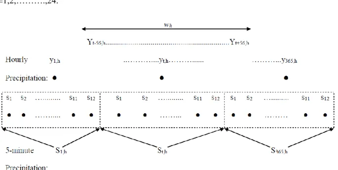
3.2.3 K-NN Hourly Disaggregation Model ... 43
3.2.4 K-NN Sub-hourly Disaggregation Model ... 46
3.2.5 Genetic Programming (GP) ... 48
3.2.6 Generalized Extreme Value Distribution and the Construction of IDF Curves ... 51
CHAPTER 4: RESULTS AND ANALYSIS... 55
4. Overview ... 55
4.1 Calibration and Validation of LARS-WG ... 55
4.2 Effect of Wet and Dry Spell Lengths ... 58
4.3 K-NN Disaggregation Model ... 64
4.3.1 Selection of Optimal Window Size... 64
4.3.2 Performance of the Disaggregation Models ... 68
4.4 Variations in the Future IDF Curves ... 74
4.4.1 Variations Obtained for CMIP5 Climate Models ... 74
4.4.2 Variations among the IDF Curves from the GP Method and the K-NN Hourly Disaggregation Model ... 78
4.5 Uncertainties in Constructing IDF Curves ... 84
4.5.1 Uncertainty due to Natural Weather Variability ... 84
4.5.2 Uncertainty due to Natural Variability and Disaggregation Models ... 85
4.5.3 Uncertainty in the Projections of Future IDF Curves ... 90
4.5.4 Uncertainty due to GEV Fitting and Extrapolation ... 92
4.6 Discussion ... 94
CHAPTER 5: SUMMARY AND CONCLUSIONS ... 96
viii
5.1 Summary of the Study ... 96
5.1.1 Downscaling of Precipitation ... 97
5.1.2 Disaggregation of Precipitation using K-NN Method ... 98
5.1.3 Comparison of K-NN and GP Methods ... 100
5.1.4 Uncertainty Analysis ... 100
5.2 Conclusions and Findings ... 101
5.3 Contribution of this Research ... 104
5.4 Limitations of the Study... 104
5.5 Future Work ... 106 References ... 107 Appendix A ... 126 Appendix B ... 128 Appendix C ... 137 Appendix D ... 143 Appendix E ... 149 Appendix F... 164
ix
LIST OF TABLES
Table 3.1: Statistics of observed daily and hourly precipitation at Saskatoon Diefenbaker Airport station during 1961-1990 ... 39 Table 4.1: Relative changes in monthly precipitation amounts between baseline and future (2020s, 2050s, and 2080s) climate as calculated from CGCM3.1 output (ratio of A1B future scenario to baseline scenario) as compared to the RCFs embedded in LARS-WG. ... 59 Table 4.2: Relative change factors for CanESM2 during 2011-2040 (RCFs during other periods are shown in Appendix B: Tables B.2 and B.3). ... 60 Table 4.3: The precipitation intensity (mm/hr) during the baseline period (1961-1990) for selected return periods. ... 76 Table 4.4: The expected precipitation intensity (mm/hr) for CanESM2 and HadGEM2-ES based on three RCPs obtained from CMIP5 during the 21st century for various return periods. ... 77 Table 4.5: Comparison between the performance of K-NN hourly disaggregation model and GP method in simulating the expected precipitation intensity (mm/hr) during the baseline period (1961-1990) for various durations and return periods. ... 80 Table 4.6: Comparison between the K-NN hourly disaggregation model and the GP method in simulating the expected precipitation intensity (mm/hr) for CanESM2 based on three RCPs during the 21st century for various durations and return periods. ... 82 Table 4.7: Historical and projected precipitation intensities for selected durations and return periods of storms in Saskatoon. Base means historical values, Min means the lowest of future projection, and Max is the highest value of future projections. The bold values represent the greatest projected change. ... 95
x
LIST OF FIGURES
Figure 1.1: Framework of the research for constructing fine-resolution IDF curves ... 9 Figure 3.1: Location of the study area (Source: Natural Resources Canada). ... 35 Figure 3.2: Location of rain gauges in Saskatoon (Source: City of Saskatoon). ... 37 Figure 3.3: Observed daily (upper panel) and hourly (bottom panel) precipitation at Saskatoon’s Diefenbaker Airport station during 1961-1990 (Source: Environment Canada) ... 38 Figure 3.4: Generation techniques of future climate change scenarios at the fine resolution (local) scale from the coarse-grid GCMs’ scale using (1) downscaling methods and (2) weather generators. ... 43 Figure 3.5: K-NN hourly precipitation disaggregation model for a typical year. ... 46 Figure 3.6: K-NN sub-hourly precipitation disaggregation model for a typical year. ... 47 Figure 3.7. Quantile-Quantile plots of the GCM-scale (using output of CanESM2) daily AMP and the local-scale daily and sub-daily AMP during the baseline (1961-1990) period in Saskatoon. ... 50 Figure 3.8: Comparison between the GEV (blue line) and empirical fit (black dots) for the local AMPs in Saskatoon with 95% confidence intervals of GEV fit shown by the red lines. ... 53 Figure 4.1: Performance of LARS-WG based on the observed monthly properties (solid lines) and 1000 realizations of synthetic (box plots) precipitation time-series during the baseline period (1961-1990) in Saskatoon. ... 56 Figure 4.2: Performance of LARS-WG based on the observed monthly properties (solid lines) and 1000 realizations of synthetic (box plots) precipitation time-series during the validation period (1991-2009). ... 58 Figure 4.3: Variations in the future projections of daily AMP quantiles in the City of Saskatoon according to CanESM2 forced with three RCPs using two sets of change factors: with wet/dry spell (blue) and without wet/dry spell (red) effects. The expected quantiles (solid lines) and their 95% confidence intervals (dashed lines) are shown with the corresponding quantiles during the baseline period (black). ... 62
xi
Figure 4.4: Boxplots of future projections of daily expected quantiles for 2-year return period precipitation in the City of Saskatoon according to CanESM2 and HadGEM2-ES forced with three RCPs using two sets of change factors, i.e. with wet/dry spell and without wet/dry spell effects along with the corresponding daily expected quantiles during the baseline. ... 64 Figure 4.5: The performance of various windows obtained for selecting optimal (green circle) window size for the K-NN hourly disaggregation model. ... 66 Figure 4.6: The performance of various windows obtained in selecting optimal (red circle) window size for the K-NN sub-hourly disaggregation model. ... 68 Figure 4.7: Performance of K-NN hourly disaggregation model based on the observed monthly properties (solid lines) and 1000 realizations of disaggregated (box plots) hourly precipitation time-series during the baseline period (1961-1990). ... 69 Figure 4.8: Performance of LARS-WG based on the observed monthly properties (solid lines) and 1000 realizations of downscaled (box plots) daily precipitation time-series during 1992-2009... 70 Figure 4.9: Performance of K-NN hourly disaggregation model based on the observed monthly properties (solid lines) and 1000 realizations of disaggregated (box plots) hourly precipitation time-series during 1992-2009. ... 71 Figure 4.10: Performance of K-NN sub-hourly disaggregation model based on the observed monthly properties (solid lines) and 1000 realizations of disaggregated (box plots) sub-hourly (5-minute) precipitation time-series during 1992-2009... 72 Figure 4.11: Performance of K-NN Sub-hourly Disaggregation Model based on the observed monthly properties (solid lines) of hourly precipitation time-series and 1000 realizations of disaggregated (box plots) 5-minute precipitation time-series (aggregated to produce hourly precipitation) during the baseline period (1961-1990). ... 73 Figure 4.12: Variations in the future IDF curves for 100-year return period in the City of Saskatoon, according to CanESM2 and HadGEM2-ES based on three RCPs. ... 75 Figure 4.13: Comparison between the future IDF curves (2011-2100) according to CanESM2 (solid lines) and HadGEM2-ES (dashed lines) based on three RCPs and 2-year return period
xii
obtained using two different downscaling approaches, i.e. GP method and LARS-WG combined with K-NN Hourly Disaggregation Model. ... 79 Figure 4.14: Theoretical GEV estimation of extreme quantiles based on the historical AMPs (black) and simulated AMPs obtained from 1000 realizations of daily precipitation time series during the baseline period using LARS-WG (red) with the corresponding 95% confidence intervals (dashed lines). ... 85 Figure 4.15: The IDF curves based on historical AMPs (black) as compared to the simulated values obtained from 1000 realizations of baseline time series from K-NN hourly disaggregation model and LARS-WG (red) with corresponding 95% confidence intervals (dashed lines). ... 86 Figure 4.16: The sub-hourly IDF curves based on observed AMPs (black) as compared to the simulated values obtained from 1000 realizations of baseline time series from K-NN hourly and sub-hourly disaggregation models and LARS-WG (red) with corresponding 95% confidence intervals (dashed lines). ... 88 Figure 4.17: Expected 1-hr AMP corresponding to 1000 realizations from LARS-WG and K-NN hourly disaggregation model (boxplot), and the same from GP method (blue dots) of 2-year return period for CanESM2 based on three RCPs during the 21st century. ... 90 Figure 4.18: Uncertainty in the projections of future extreme precipitation quantiles for 2-year return period based on two GCMs and three RCPs obtained from CMIP5 and quantified by using GEV shown as 95% confidence intervals (dashed lines) with expected quantiles (solid lines). .. 92 Figure 4.19: Uncertainty in the projections of future extreme precipitation quantiles for 2-, 5-, 25- and 100-year return periods based on two GCMs and three emission scenarios obtained from CMIP5 and quantified by using GEV shown as 95% confidence intervals (dashed lines) using 90 years of data (2011-2100) with expected quantiles (solid lines). ... 93
xiii
LIST OF SYMBOLS AND ABBREVIATIONS
AAFC-WG Agriculture and Agri-Food Canada Weather Generator
ACCESS1.0 Australian Community Climate and Earth-System Simulator 1.0 AMP Annual Maximum Precipitation
ANN Artificial Neural Network
AOGCM Atmospheric Ocean General Circulation Model
AR4 Fourth Assessment Report
AR5 Fifth Assessment Report
BCCCSM1.1 Beijing Climate Center Climate System Model 1.1 CanESM2 Second generation Canadian Earth System Model CCCMA Canadian Centre for Climate Modelling and Analysis CDCD Canadian Daily Climate Data
CESM1-BGC Community Earth System Model, version 1-Biogeochemistry CGCM3 The third generation Coupled Global Climate Model
CHRM Climate High Resolution Model
CMIP3 Coupled Model Intercomparison Project, phase 3 CMIP5 Coupled Model Intercomparison Project, phase 5
CO2 Carbon dioxide
CRCM Canadian Regional Climate Model
CSIRO-Mk3.6.0 Commonwealth Scientific and Industrial Research Organization, Mk3.6.0 version
ECDF Empirical Cumulative Distribution Function
xiv
GCM Global Climate Model
GEV Generalized Extreme Value
GLM Generalized Linear Model
GLM-WG Generalized Linear Model-based Weather Generator
GP Genetic Programming
GSR Genetic Symbolic Regression
HadCM3 Hadley Centre Coupled Model, version 3
HadGEM2-ES The Earth System configuration of the Hadley Centre Global Environmental Model, version 2
HadRM Hadley Center Regional Model IAM Integrated Assessment Model
IDF Intensity-Duration-Frequency
INM-CM4 Institute of Numerical Mathematics Climate Model, version 4.0 IPCC Intergovernmental Panel on Climate Change
K-NN K-Nearest Neighbor
KS-test Kolmogorov-Smirnov test
LARS-WG Long Ashton Research Station Weather Generator MARE Mean Absolute Relative Error
MB Mean Bias
MIROC-ESM Model for Interdisciplinary Research on Climate-Earth System Model MM5 Fifth Generation Pennsylvania State University/National Center for
Atmospheric Research Mesoscale Model
MRI-CGCM3 Meteorological Research Institute-third generation Coupled Global Climate Model
xv R Pearson’s correlation coefficient
RCF Relative Change Factor
RCM Regional Climate Model
RCP Representative Concentration Pathway RegCM Regional Climate Model System
RMSE Root Mean Squared Error
SDSM Statistical Downscaling Method
SED Semi-Empirical Distribution
SRES Special Report on Emission Scenarios
WGEN Weather Generator
1
CHAPTER 1: INTRODUCTION 1.1 Background
The use of Intensity-Duration-Frequency (IDF) curves, which incorporate the frequency and intensity of maximum precipitation events of various durations for the design of hydrosystems, is standard practice in many places. The amounts of maximum daily and sub-daily precipitation values, similar to those represented by IDF curves, have shown increasing trends in many locations of the world including Canada (Arnbjerg-Nielsen, 2012; Denault et al., 2002; Waters et al., 2003). The return period of a particular precipitation event (i.e., storm) is subject to change over time as a result of non-stationarity (Mailhot and Duchesne, 2010). The Intergovernmental Panel on Climate Change, IPCC (2012) concluded that the return period of a given Annual Maximum Precipitation (AMP) amount will decrease significantly by the end of the 21st century, with the occurrence of extreme precipitation events occurring more frequently. For example, if an urban storm water collection system was designed 30 years ago based on the 50-year 10-min precipitation storm, the design might only satisfy up to a 25-year design storm under non-stationary climatic conditions. Such conditions may significantly increase the vulnerability of urban storm water collection systems, which are associated with design-storm durations of less than a day and even less than an hour in many cases.
Understanding of the dynamics of hydrological processes and their impacts on urban storm water collection system requires a long record of fine resolution precipitation (Segond et al., 2006), but records of fine temporal and spatial resolution are often limited. Many regions have precipitation records at daily scale with limited hourly records in the world. Obtaining sub-hourly precipitation records has become an important issue as climate change has been shown to cause increased precipitation intensities in many parts of the world, including Canada (Waters et
2
al., 2003). Global Climate Models (GCMs) have the ability to represent weather variables at coarse grid scale (usually greater than 200 kilometers), which is too coarse for climate change impact studies (Mladjic et al., 2011; Nguyen et al., 2008), especially in urban hydrology where the required scale is usually less than a few kilometers. The GCMs’ outputs are usually downscaled to the local scale using various downscaling methods; for instance, weather generators, such as Long Ashton Research Station Weather Generator (LARS-WG) (Racsko et al., 1991; Semenov and Barrow, 1997) to obtain required information for impact investigations.
LARS-WG is a semi-parametric, widely used and user-friendly weather generator, where precipitation and other outputs of GCMs can be downscaled to local scale (a scale of influence for hydrological processes and infrastructure) using the statistical properties of the observed weather at the local scale (Semenov and Barrow, 1997). In LARS-WG, the observed precipitation data are used to obtain the distribution of wet and dry spell lengths of the simulated series (King et al., 2012). Since the collection of fine resolution observations is not an easy option, transformation of the available data from one temporal and spatial scale to another is an important alternative (Sivakumar et al., 2001). The transformation of precipitation data from one scale to another can be achieved through the application of disaggregation models for transforming daily precipitation to hourly and to sub-hourly values.
The share of rainfall in the monthly precipitation showed significant increasing trends in a number of location in the Canadian prairies, when investigated using the historical data from the Historical Adjusted Database for Canada (HACDC) (Shook and Pomeroy, 2012). Several researchers have concluded that based on the simulation results of GCMs, a warmer climate is expected in Saskatchewan, Canada, on a regional scale (Lapp et al., 2008), which will ultimately intensify the hydrological cycle (Trenberth et al., 2003). In Saskatoon, the frequency and mean
3
value of daily precipitation quantities for late spring and summer seasons, specifically in June and July, show a significant increasing trend in the 21st century as revealed from the preliminary
study based on Saskatoon’s Airport historical precipitation data, five GCMs, and three emission scenarios (Nazemi et al., 2011). Depending on the GCMs and the emission scenarios, the amount of increase would vary; this suggests that uncertainty cannot be avoided in future climate projections and that uncertainty quantification measures should be associated with each projection so that the likelihood of future precipitation events might be quantified.
Saskatoon’s storm water collection system consists of minor and major sub-systems (City of Saskatoon, 2012). The minor systems are designed to withstand storm events of either 2 or 5-year return periods, whereas the major systems must control peak runoff of a 100-5-year return period. The City of Saskatoon currently uses the IDF curves based only on historical data up to 1986, assuming that the future will behave like the past. Nevertheless, recent (2010) total spring and summer precipitation was record breaking, being almost 50% larger than the previous highest levels observed since the 1920s. Manitoba and Saskatchewan recorded the second highest losses of roads, houses, farms, and animals in Canadian history due to disasters caused by weather extremes after 2005 (Environment Canada, 2011). Evacuation and relocation of several communities had to be implemented as a result of higher water levels, as compared to the water levels in 2005 (Massie and Reed, 2012). The floods in the recent years were caused by the heavy spring precipitation, as a sum of rainfall and snow, when rivers are already in high flow situations (Environment Canada, 2011). This increase in precipitation and river water levels reveals that extreme events might not be following historical frequencies. The wet summers of recent years, supported by other regional studies of climate change, emphasizes the need to
4
investigate possible changes in the IDF curves and design storms in Saskatoon as a result of possible climate change.
1.2 Area of Interest
It is often necessary to downscale precipitation from the global coarse spatial scale to the local scale and to finer timescales for the study of climate change in urban areas. Hourly and even sub-hourly future precipitation scenarios are required for accurate modeling of hydrological response of urban drainage catchment (Watt et al., 2003), since urban drainage system involves a small catchment as compared to the natural catchments (Schilling, 1991). Therefore, disaggregation of precipitation to fine temporal and spatial resolutions is required to assess the vulnerability of storm water collection systems in urban areas. A stochastic weather generator (e.g., LARS-WG) is capable of producing an ensemble of future daily weather series at the local-scale based on the GCMs’ predictions, which also provides the means for exploring uncertainty in climate change projections (Semenov and Stratonovitch, 2010). The stochastic weather generator can also be used to assess the effects of wet and dry spell lengths on the simulations, in addition to the effects of mean monthly precipitation amounts.
A method was sought to disaggregate the daily precipitation to finer temporal resolution, while maintaining the statistical properties of the observed precipitation. The K-nearest Neighbor (K-NN) method, based on the resampling algorithm from true observed data, so that statistical properties of the disaggregated precipitation series have a high probability of being preserved, was selected. The K-NN method can be used as a disaggregation model to generate long time-series of hourly and sub-hourly (5-minute) precipitation for the baseline (historical) period as well as the future climate projections. Afterwards, the long recorded data of hourly and
sub-5
hourly (5-minute) precipitation can be further analyzed to construct the IDF curves during the baseline and future periods (i.e., 2011-2100) for the City of Saskatoon.
The two-stage downscaling and disaggregation method can be applied to construct future IDF curves of all durations between 5 minutes and 24 hours; allowing the current IDF curves to be updated for the City of Saskatoon. Several previous studies related to IDF curves considered generation of annual maximum precipitation (Kuo et al., 2013; Hassanzadeh et al., 2013). Typically, the generation of continuous precipitation records has not been extensively considered in previous studies. However, long continuous precipitation time series (not only daily/annual maximum) of 5-minute resolution during the baseline and future periods might be important to represent high resolution extreme precipitation quantiles in the prairie region where precipitation during the summer months occurs mostly as convective precipitation (Shook and Pomeroy, 2012). Some previous studies used the K-NN method as a weather generator to produce daily precipitation by resampling from the observed daily precipitation data (Sharif and Burn, 2007) and as a disaggregation model to disaggregate daily to hourly precipitation values (Prodanovic and Simonovic, 2007) using a prescribed window size described by Yates et al. (2003). However, window size (number of nearest neighbors) needs to be examined for the hydrological system in Saskatoon for the K-NN hourly and sub-hourly disaggregation models; and two optimal windows can be selected separately for the two disaggregation models. The optimal window size for disaggregation models has not been thoroughly investigated in previous studies. Furthermore, the selection of nearest neighbors, either randomly or deterministically, needs verification when there are several neighbors showing the same minimum distance from the point of interest. A general and user-friendly method is needed, which can be applied to any location using precipitation output from any GCM.
6
Applying the above-mentioned two stage downscaling/disaggregation method, while identifying the optimal window size for the K-NN method and quantifying the various sources of uncertainties associated with developing the IDF curves for the City of Saskatoon, is the main area of interest in this thesis.
1.3 Knowledge Gap
Currently, there is no up-to-date study investigating the possible changes in the IDF curves and design storms in the City of Saskatoon under climate change or non-stationarity. The risk and rate of failure of systems designed using the historical design storms may increase in the face of non-stationary climatic conditions (Mailhot et al., 2007; Adamowski et al., 2009).
Characterization of the possible future changes in short-duration precipitation intensities faces several obstacles and appropriate methods need to be developed for this purpose. First, the short-duration precipitation events in the Canadian prairies, which includes Saskatoon, are mostly convective during the summer months (Shook and Pomeroy, 2012). Therefore GCM simulations might be insufficient to reproduce the precipitation for a small area (Olsson et al., 2009). Second, the outputs of GCMs for a given site and time period vary tremendously among various GCMs and representative concentration pathways (RCPs)/emission scenarios. However, no GCM can be preferred without a detailed study (Semenov and Startonovitch, 2010). Moreover, the outputs of GCMs are not available for durations shorter than a day in case of CMIP3 climate models, or several hours in case of CMIP5 climate models. The uncertainty due to the choice of GCMs requires multi-model ensembles of climate projections with several modeling alternatives for characterizing future precipitation events. Furthermore, hourly and even sub-hourly future precipitation scenarios are required for accurate modeling of the hydrological response of urban watersheds. Therefore, disaggregation of precipitation to fine
7
temporal resolutions should be performed to assess the vulnerability of storm water collection systems in the City of Saskatoon with an estimation of uncertainty associated with the constructed IDF curves and the subsequent hydrological risks. This study is part of a sole source project funded by the City of Saskatoon to fill the above-identified knowledge gap.
1.4 Objectives
The goal of this research project is to construct the Intensity-Duration-Frequency (IDF) curves/design storms for the City of Saskatoon under climate change scenarios. The specific objectives are the following:
(1) To generate representative long time series of hourly and sub-hourly precipitation for the City of Saskatoon, during the baseline period and under projections of climate change scenarios;
(2) To construct a set of potential future IDF curves for design purposes in Saskatoon; and (3) To assess and quantify the uncertainties in the constructed IDF curves.
1.5 Scope of the Research
This research study aims to investigate the difference among GCMs available for AR5 (phase 5 of the Coupled Model Intercomparison Project: CMIP5 archive) based on representative concentration pathways (RCPs) and AR4 (phase 3 of the Coupled Model Intercomparison Project: CMIP3 archive) scenarios of CO2 emissions on future hourly and sub-hourly
precipitation in the City of Saskatoon. GCMs provide the basis for characterizing the effects of CO2 emissions and management strategies on general circulation patterns in large temporal and
spatial scales. As the outputs of GCMs are not directly applicable to small temporal and spatial scales, it is therefore necessary to downscale the future realizations of precipitation time series generated by GCMs using downscaling techniques. In this study, LARS-WG was used as one of
8
the available downscaling techniques to map the projections of GCMs from the coarse grid resolution to a local scale and to generate multiple realizations of future daily precipitation. Two GCMs, the Canadian CanESM2 and the British HadGEM2-ES were considered in this study. Then, a disaggregation technique was employed to further downscale the generated daily local precipitation data into hourly and sub-hourly values for the city. Figure 1.1 shows the framework of the research being conducted under this study. Other GCMs’ and Regional Climate Models’ (RCMs) simulations are not within the scope of this research study.
This research study uses a stochastic weather generator, LARS-WG, which uses historical daily precipitation data to estimate parameters of the empirical probability distributions of daily precipitation. The outputs of GCMs are used to update the parameters of the distributions and the updated parameters are then used to generate future daily precipitation series under climate change scenarios. An hourly disaggregation method disaggregates historical or future daily precipitation to the historical or future hourly precipitation data by sampling from the historical hourly precipitation time series. Similarly, a sub-hourly disaggregation method disaggregates historical or future hourly precipitation to historical or future sub-hourly precipitation data by sampling from the historical sub-hourly precipitation time series. The disaggregated precipitation time series, both historical and future, are then used to construct the historical and future IDF curves of fine resolutions. Genetic Programming is employed to find equations that expresses the relationship between the global scale daily precipitation quantiles, and local scale daily and sub-daily precipitation quantiles during the baseline period. These equations are then used to find local scale future precipitation quantiles and IDF curves using the global scale future quantiles. Changes in the future IDF curves are assessed relative to the historical IDF curves.
9
Figure 1.1: Framework of the research for constructing fine-resolution IDF curves
1.6 Synopsis of the Thesis
The rest of this thesis is organized in the following chapters. Chapter 2 provides a concise literature review on Global Climate Models (GCMs); various downscaling approaches; dynamic and statistical downscaling methods, including stochastic weather generators and LARS-WG;
Stochastic weather generator (LARS-WG) GCMs’ outputs
Historical daily data
Future daily precipitation scenarios
Hourly disaggregation
Future hourly precipitation scenarios using GP
Future IDF curves using GP Hourly precipitation data Sub-hourly disaggregation Sub-hourly precipitation data Future fine-scale IDF
curves/design storms Historical IDF
curves/design storms
Comparisons
10
IDF curves under the projections of climate change; generation of high resolution spatial and temporal precipitation time series; K-nearest Neighbor (K-NN) method; and Extreme Value statistical distributions. Chapter 3 presents the case study and data and methods used in this thesis. Chapter 3 also provides a description of the K-NN hourly and sub-hourly disaggregation models and the two-stage downscaling/disaggregation method. Chapter 4 presents results and analysis of LARS-WG, K-NN hourly and sub-hourly disaggregation models; analysis of variations in the IDF curves obtained using the proposed two-stage modeling method and another existing method; variations in the future fine-resolution IDF curves; different sources of uncertainty; and uncertainties in the construction of future IDF curves. Finally, chapter 5 presents a summary, conclusions, research contributions, limitations of the study, and recommendations for future studies.
11
CHAPTER 2: LITERATURE REVIEW 2. Overview
The research proposed for this thesis requires the development of a two-stage downscaling and disaggregation method to create IDF curves for the study area, Saskatoon, Canada, under the baseline period and under the projections of climate change scenarios using the precipitation output from selected Global Climate Models (GCMs). This chapter presents a literature review of the following important components of this study: (1) global climate models, (2) downscaling methods, (3) precipitation disaggregation methods, (4) extreme value distribution models, (5) construction of future fine-resolution IDF curves, and (6) uncertainty estimation related to the IDF curves.
2.1 Global Climate Models
Assessment of climate change is primarily based on General Circulation Models or Global Climate Models (GCMs). The GCMs are numerical models that can represent physical processes in the atmosphere, ocean, cryosphere and land surface. Currently, it is considered that the only scientifically sound way to predict the impact of increased greenhouse gas emissions on the global climate is through global scale simulation (Barrow, 2002). GCMs can simulate the responses of the global climate to increasing greenhouse gas concentrations (Taylor et al., 2012; Moss et al., 2010). GCMs can incorporate the three-dimensional nature of atmosphere and ocean, simulating as many processes as possible by coupling of atmosphere-ocean GCMs (AOGCMs) with the inclusion of changes in biomes, atmosphere, ocean, and even soil chemistry (McGuffie and Henderson-Sellers, 2014). AOGCMs are the physical climate models with high complexity, whereas the physical climate models with intermediate complexity, known as Earth System Models (ESM), can account for the major carbon fluxes among the ocean, atmosphere, land and
12
vegetation carbon reservoirs for long-term climate modeling (Moss et al., 2010; Taylor et al., 2012). In this study, the precipitation output from two ESMs (CanESM2 and HadGEM2-ES) was considered for the long term (2011-2100) impact assessment of climate change in Saskatoon.
Previously, the GCMs’ simulations of climate variables based on three emission scenarios (SRES: A1B, A2, and B1) from the Coupled Model Intercomparison Project Phase 3 (CMIP3) were commonly used. The Fourth Assessment Report (AR4) of the Intergovernmental Panel on Climate Change (IPCC) was supported by CMIP3 and the outputs of climate models included in CMIP3 have been the basis of climate change impact studies conducted by the research community around the world since 2007 (IPCC, 2007; Taylor et al., 2012). The outputs of climate models from CMIP3 provided comprehensive multi-model impact assessment for climate change projections during the 21st century, based on the IPCC Special Report Emission Scenarios (SRES), i.e., A1B, A2, and B1. Scenarios describe plausible trajectories of the future climate conditions (Moss et al., 2010) and perform as an appropriate analytical tool to assess the influence of driving forces on future emission results and associated uncertainties (IPCC, 2007). A1B, A2 and B1 scenarios represented “a rich world”, “a very heterogeneous world”, and “a convergent world”, respectively (for details please refer to Nakicenovic et al., 2000). The GCMs’ outputs were contributed by some modeling centers and archived in the Program for Climate Model Diagnosis and Intercomparison (PCMDI) (http://www-pcmdi.llnl.gov/).
With the release of the Fifth Assessment Report (AR5) of IPCC based on Phase 5 (CMIP5), a new set of GCM simulations was made freely available to the research community. CMIP5 climate models produce a comprehensive set of outputs with the inclusion of new emission scenarios, known as Representative Concentration Pathways (RCPs) (Moss et al., 2010; Taylor et al., 2012). With the introduction in September 2013 of AR5 based on CMIP5, updating
13
the previous simulations of projected climate change based on CMIP3 climate models became a requirement. Generally, CMIP5 includes more than 50 sophisticated climate models (GCMs) from more than 20 modeling groups and a set of new forcing scenarios (Taylor et al., 2012). Examples of these GCMs include: ACCESS1.0, BCC-CSM1.1, CanESM2, CESM1-BGC, CSIRO-Mk3.6.0, HadGEM2-ES, INM-CM4, MIROC-ESM and MRI-CGCM3 (CMIP5, 2013). The new scenarios used in the simulations of climate models (GCMs) in CMIP5 are known as Representative Concentration Pathways (RCPs). The policy actions to achieve a wide range of mitigation were included in the RCPs aiming to have different radiative forcing targets by the end of the 21st century. The RCPs are denoted by the approximate radiative forcing they might reach by the end of the 21st century, as compared to the year 1750: i.e., RCP2.6, RCP4.5, RCP6.0, and RCP8.5 denote the target radiative forcings of 2.6, 4.5, 6.0 and 8.5 Wm-2, respectively (IPCC, 2013). The values of radiative forcing represented by each RCP are indicative of the targets only by the end of year 2100. However, a range of 21st century climate policies can be represented by the RCPs as compared with the no-policy AR4 emission scenarios. The relative projections due to AR4 and AR5 emission scenarios/RCPs are shown in Appendix A (Figures A.1 and A.2).
The Integrated Assessment Models (IAMs) were used by the Integrated Assessment Modeling Consortium (IAMC) to produce the RCPs by considering various components such as demographics, economics, energy, and climate (IPCC, 2013). Generally, IAMs combine a number of component models, which mathematically represent findings from different contributing sectors. IAMs are broadly of two categories: policy optimization models and policy evaluation models (Weyant et al., 1996). Policy alternatives for the control of climate change can be evaluated by combining technical, economic and social aspects of climate change in an IAM
14
(Kelly and Kolstad, 1998). In this study, the precipitation output from two GCMs (CanESM2 and HadGEM2-ES) and the corresponding three RCPs (RCP2.6, RCP4.5, and RCP8.5) were considered.
2.2 Downscaling Methods
Assessment of climate change is primarily based on outputs from GCMs, although the climate variables at the local scale – scale of influence for hydrological processes and infrastructure – show large differences when compared with those at the coarse scale of GCMs (Zhang et al., 2011; Hashmi et al., 2011). To overcome this problem, various downscaling approaches are usually used, and they are broadly in two categories: dynamical and statistical downscaling methods (Hashmi et al., 2011; Franczyk and Chang, 2009). A brief description of these downscaling methods is provided in the following sections.
2.2.1Dynamical Downscaling
Dynamical downscaling is performed by running Regional Climate Models (RCMs) at fine scales using the outputs of GCMs (Xue et al., 2014; Sharma et al., 2011) as boundary conditions. Originally, RCMs were developed as physically based downscaling tools; currently, however, their use for simulating physical processes has been increased (Giorgi and Mearns, 1999; Frei et al., 1998). Examples of RCMs include the Canadian regional climate model (CRCM), climate high-resolution model (CHRM), Hadley Center regional model (HadRM), regional climate model system (RegCM), and the Fifth Generation Pennsylvania State University/National Center for Atmospheric Research mesoscale model (MM5). Typically, high-resolution (10-50 km) RCMs are nested within the coarse high-resolution (typically greater than 200 km) GCMs for the purpose of dynamical downscaling, although the use of RCMs as a downscaling tool is computationally expensive.
15
Downscaling RCM outputs employs bias correction as biases in the GCMs’ and RCMs’ simulations restrict their direct use in climate change impact studies, which need what is known in the literature as “bias correction”. In the simulations of RCMs, the biases could be due to the improper boundary conditions provided by the GCMs, lack of consistency in the representation of physics between GCMs and RCMs, and parameterizations of RCMs (Ehret et al., 2012). Out of many bias-correction methods available in the literature, the following list only provides a glimpse of them: correction of monthly mean (Fowler and Kilsby, 2007), delta change method (Hay et al., 2000; Olsson et al., 2012a), and quantile-based method (Kuo et al., 2014; Sun et al., 2011).
Biases in the output of RCMs may be overcome and/or reduced to some extent, if not fully, through improving the model predictability, use of multi-model ensembles of GCMs and/or RCMs (to estimate uncertainty bounds), and by processing the model output afterwards (Ehret et al., 2012). Fowler and Kilsby (2007) applied a simple monthly mean correction to the mean monthly precipitation from RCM (HadRM3H) and found it an effective method to estimate observed precipitation variability during the baseline period. They preferred this simple correction method to a complex quantile-based method (used by Wood et al., 2004) as a reasonable estimate of the observed climate variability was provided by the simple method with slight underestimation of the variability due to simplification of the method. Their method used probability distributions for correcting model bias and assumed that they will remain stable over time, which may not be the case in reality.
Olsson et al. (2012a) demonstrated how precipitation from RCM projections can be further downscaled using the delta change approach to fine resolutions in time and space suitable for the impact assessment of climate change on urban hydrology. The delta change approach
16
(also known as change factor) has been widely used and applied in climate change impact studies in many different ways, one of which is the multiplicative change factor. The multiplicative change factor (also called relative change factor) is the ratio between the future and the baseline simulations obtained from GCMs, which is then multiplied by the observed data (e.g., precipitation) to generate climate change scenarios of precipitation at the local scale (Anandhi et al., 2011). Kuo et al. (2014) concluded that the IDF curves constructed with bias corrected MM5 precipitation data using a quantile-based method were consistent with the IDF curves at the rain-gauges in Edmonton. Sharma et al. (2011) used statistical downscaling method (SDSM) and a data-driven technique for downscaling the RCM data; they found that the further downscaled data were closer to the observed data than the raw RCM data.
2.2.2Statistical Downscaling
Statistical downscaling is based on the statistical relationship between the GCMs’ outputs and the local scale observed data (e.g., precipitation) (Wilby et al., 1998). Statistical downscaling may be classified into three sub-types: weather typing approaches, regression-based methods and stochastic weather generators (Wilby and Wigley, 1997).
(i) Weather Typing Approaches
Local meteorological data are categorized by weather type according to the patterns prevailing in the atmospheric circulation. Mean precipitation, or the entire precipitation distribution, is associated with a particular weather type of large-scale variables provided by GCMs. The downscaling method is founded on the relationships between the large-scale climate variables (predictor) and local scale observed weather variables (predictand). However, instead of creating a continuous relationship between the variables, local scale climate variables (e.g., precipitation) are generated either by resampling from the observed data distribution conditioned
17
on the atmospheric circulation patterns given by GCMs, or by producing sequences of local scale weather patterns by the Monte Carlo simulation method and then resampling from the observed data (Wilby and Dawson, 2004). To downscale a future daily precipitation event produced by a GCM, an analogous condition is searched in the observed data of climatic variables, and the local scale observed precipitation for the same event is selected as downscaled future precipitation. Generally, pressure fields produced by GCMs are used as predictors, so weather types are classified using a classification scheme based on the pressure fields.
The weather typing downscaling method prevents the selection of an extreme future precipitation event beyond the most extreme events in the historical records, only allowing the modification of the sequence and frequency of historical precipitation. However, this limitation can be overcome if changes in the atmospheric circulation are considered along with changes in other atmospheric predictors (e.g., temperature, humidity) (Willems et al., 2012; Wilby and Dawson, 2004). Willems and Vrac (2011) compared the performance of a weather typing downscaling method with that of a quantile-perturbation based method (based on quantiles) in terms of changes in the IDF curves in Belgium. The changes in short-duration precipitation extremes were produced similarly by the two methods with the weather typing method using temperature as a large-scale predictor (in addition to atmospheric circulation).
(ii) Regression-based Methods
Regression-based methods are also known as transfer function methods; they involve developing relationships between the local scale (i.e., point station) variables (i.e., precipitation) and global scale (i.e., GCM) variables. Several studies have used regression-based downscaling techniques, such as multiple linear regression (Wilby et al., 2002; Jeong et al., 2012), generalized linear models (GLM) (Chun et al., 2013; Yang et al., 2005; Chandler and Wheater, 2002),
18
canonical correlation analysis (Busuioc et al., 2008; Von Storch et al., 1993), artificial neural networks (Schoof and Pryor, 2001; Hewitson and Crane, 1996), and the genetic programming-based method (Hassanzadeh et al., 2014).
Artlert et al. (2013) used the SDSM, a multiple regression-based statistical downscaling model (Wilby et al., 2002), to establish a relationship between the GCM-scale climate simulations and local scale precipitation characteristics. They analyzed future precipitation characteristics based on projected trends from the British GCM (HadCM3) and the Canadian CGCM3, which showed huge differences between the future precipitation projections by the two GCMs. The differences in future precipitation projections indicate a high uncertainty in the GCM-based climate simulations. The precipitation data obtained through downscaling are also uncertain, depending on the GCMs and downscaling methods used (Willems et al., 2012). Jeong et al. (2012) used a hybrid downscaling approach as a combination of regression-based (multiple linear regression) and stochastic weather generation techniques to simulate precipitation at multiple sites in southern Quebec, Canada. They found that the addition of a stochastic generation approach to the multivariate multiple linear regression method improved the performance of downscaling daily precipitation from the Canadian CGCM3. The use of a hybrid downscaling approach can overcome the shortcomings of multivariate multiple linear regression and stochastic generation approaches when they are used separately. Yang et al. (2005), and Chandler and Wheater (2002) used the GLM framework for generating daily precipitation sequences conditioned upon several external predictors; this offers superiority in simulating non-stationary sequences, since the external predictors may have spatial and temporal variations.
Hewitson and Crane (1996) applied Artificial Neural Networks (ANNs) for learning the linkage between the atmospheric circulation produced by GCMs and the local scale precipitation.
19
The ANNs were trained for each rain gauge station to predict daily precipitation values using the linkage learned by the ANNs. However, ANNs end up in generalized relationships, which always predict the same precipitation for a given circulation. Chadwick et al. (2011) used ANNs to reproduce temperature and precipitation dynamically downscaled by nested RCM within a GCM in Europe and concluded that ANNs were capable of reproducing the corresponding climate variables but missed high precipitation values over some mountain areas. The ANNs trained with only 1960-1980 data were not able to reproduce temperature or precipitation well for the 1980-2000 or 2080-2100 periods, although their performance was improved by training the ANNs using different time periods. The GP-based quantile downscaling (Hassanzadeh et al., 2014) is a novel type of statistical downscaling method because it maps the relationship between extreme precipitation (quantiles) at both the global and local scale without having to generate a continuous precipitation record. GP has the advantage of producing explicit mathematical equations for the downscaling relationship.
(iii) Stochastic Weather Generators and LARS-WG
Quantification of the uncertainty due to internal natural weather variability based on stochastic weather generators has a number of applications in design and/or operation of many systems, such as water resources systems, urban drainage systems and land management changes (Srikanthan and McMahon, 2001). Historically, efforts were made to describe precipitation processes in constructing weather generators, since precipitation is the most critical climate variable for many applications, and very often its value is precisely zero (Wilks and Wilby, 1999). The process of precipitation occurrence describes two states, wet and dry, which forces many weather generators to model separately the occurrence and intensity of precipitation.
20
The first statistical model for simulating the occurrence of daily precipitation was developed by Gabriel and Neumann (1962) using a first-order Markov Chain model. They assumed that the probability of precipitation occurrence is conditioned only on the weather condition of the previous day, i.e., wet or dry. Later, the first-order Markov Chain model of daily precipitation occurrence was combined with a statistical model (i.e., exponential distribution) of daily precipitation (with nonzero value) amounts by Todorovic and Woolhiser (1975). These initial models were constructed for the simulation of a single climate variable, generally daily precipitation for hydrological analysis. The simulation of other climate variables (e.g., daily precipitation, temperature and solar radiation) became reasonable using stochastic weather generators in the early 1980s, which were developed by Richardson (1981) and Racsko et al. (1991). Climate change has increased interest in stochastic weather generators for stochastic simulation of local weather (Semenov and Barrow, 1997).
A stochastic weather generator is used to simulate a daily time series of weather variables having statistical characteristics similar to observed weather variables (Wilks and Wilby, 1999). Various tools (Semenov and Barrow, 1997; Wilks, 1999; Wilks and Wilby, 1999; Wilby and Dawson, 2007; Sharif and Burn, 2007; Hundecha and Bardossy, 2008; King et al, 2014) have been proposed as weather generators. Multiple regression models and stochastic weather generators are examples of the statistical downscaling techniques that are widely used (Wilks, 1992, 1999), since they are less computation intensive than other downscaling methods, easy to use, and efficient (Semenov et al., 1998; Dibike and Coulibaly, 2005). Hashmi et al. (2011) conducted a comparison between a multiple regression-based model (i.e., SDSM) (Wilby et al., 2002) and a weather generator (i.e., LARS-WG), which showed their (SDSM and LARS-WG)
21
acceptability with reasonable confidence as downscaling tools in climate change impact assessment studies.
Two weather generators, LARS-WG and the Agriculture and Agri-Food Canada weather generator (AAFC-WG), were used by Qian et al. (2008) to reproduce daily extremes (maximum daily precipitation, the highest daily maximum temperature and the lowest daily minimum temperature) over the period 1971-2000. Both weather generators were found to reproduce extreme daily precipitation values quite satisfactorily, while LARS-WG was found to perform better in preserving the historical statistics (e.g., absolute maximum and minimum temperature, mean and standard deviation of precipitation) (Irwin et al., 2012). Chun et al. (2013) compared the downscaling abilities of LARS-WG and GLM-based weather generator (GLM-WG) (Chandler and Wheater, 2002) using the climate variables during the baseline (1961-1990) and future (2071-2100) periods. GLM-WG, a stochastic precipitation model, was developed based on the GLM structure and two-stage precipitation model (first, modeling the sequence of wet/dry days using logistic regression and second, modeling the precipitation amount using gamma distributions) (Coe and Stern, 1982). LARS-WG uses observed daily precipitation to generate synthetic daily precipitation series at a specific site (Semenov and Barrow, 2002), while GLM-WG simulates daily precipitation based on large-scale climate information at a particular time and location (Chandler and Wheater, 2002). In that particular study by Chun et al. (2013), both weather generators showed equal performance in simulating monthly and annual precipitation totals, while GLM-WG showed superiority in simulating annual daily maximum precipitations due to the large-scale climate information used in GLM-WG.
Qian et al. (2004) and King et al. (2012) concluded that LARS-WG performed better in simulating daily precipitation, but its performance in simulating temperature related statistics
22
(e.g., absolute maximum and minimum temperature) was not adequate when compared to the corresponding performances of AAFC-WG, SDSM, and K-NN weather generators with Principal Component Analysis (WG-PCA). However, LARS-WG was found to perform well in simulating climatic extremes across Europe (Semenov and Barrow, 1997). The IPCC’s Fourth Assessment Report (AR4) (Solomon et al., 2007) used a multi-model ensemble, out of which 15 climate models have been incorporated in the new version (Version 5) of LARS-WG for climate projections. The model ensemble allows estimation of uncertainties associated with the impacts of climate change originating from uncertainty in climate predictions (Semenov and Stratonovitch, 2010).
Several studies using LARS-WG for climate change impact assessment (Semenov and Barrow, 1997) suggested that LARS-WG can be used as a downscaling model with substantial confidence to conduct climate change impact assessment by extracting site-specific climatic characteristics (Hashmi et al., 2011; Semenov and Stratonovitch, 2010; Qian et al., 2008; Semenov and Barrow, 1997). LARS-WG can be used to generate synthetic daily precipitation data by calculating site-specific weather parameters from observed daily data of at least 20 years (Semenov and Barrow, 1997). The LARS-WG is capable of producing daily climate scenarios for the future at the local scale based on the GCMs’ predictions and emission scenarios, thus providing the means for exploring the uncertainty in climate change impact assessment (Semenov and Stratonovitch, 2010).
LARS-WG was adopted for this research as a stochastic weather generator tool to simulate climate data (e.g., temperature, precipitation) in Saskatoon, Canada, during the baseline period and under future climatic conditions. LARS-WG was employed in this research for generating multiple realizations of daily precipitation at the local scale in Saskatoon. LARS-WG
23
provides a computationally inexpensive platform for generating daily future climate data (e.g., temperature, precipitation) for many years under the projections of climate change scenarios, which are of spatial and temporal resolution suitable for local scale climate change impact studies. LARS-WG can reproduce changes in the mean climate, and in the climate variability at the local scale. The first version of LARS-WG was developed in 1990; the latest version was developed in 2002, incorporating a series approach (Racsko et al., 1991), which in this context means that the weather generation begins with the simulation of wet/dry spell length and then the precipitation amount is modelled (Semenov and Barrow, 2002). The performance of LARS-WG was compared with the performance of another popular stochastic weather generator, WGEN (Richardson, 1981), over several sites with diverse climates and was found to perform as well as WGEN (Semenov et al., 1998).
The weather generation process in LARS-WG is based on semi-empirical distribution (SED), which is defined as the cumulative probability distribution function describing the probability that a random variable X, with a given probability distribution, takes on a value less than or equal to x. The empirical distribution is represented by a histogram with 23 semi-closed intervals, [ai-1,ai), where ai-1, ai indicates the number of events in the observed data in the
i-th interval and i=1,2,……..,23. The values of the events are selected randomly from the semi-empirical distributions, where an interval is selected first using the fraction of events in every interval as the probability of choice; subsequently, a value is chosen from that interval using a uniform distribution. SED provides a flexible distribution with a possibility to approximate a wide range of shapes through adjustment of the intervals, [ai-1,ai). The choice of the intervals, [a i-1,ai) is dependent on the weather variable type; for example, the intervals are evenly spaced in
24
spell lengths and for precipitation in order to restrict the use of very coarse resolution intervals for extremely small values (Semenov and Stratonovitch, 2010; Semenov and Barrow, 2002). More explanation of the steps for generating daily precipitation time-series using LARS-WG is provided in Appendix B (Section B.1).
2.3 Precipitation Disaggregation Methods
To overcome the lack of high-resolution temporal and spatial precipitation data crucial for hydrological, meteorological and agricultural applications, disaggregation of available data from one temporal and spatial scale to another seems to be the most efficient alternative (Sivakumar et al., 2001). Several disaggregation techniques exist in water resources literature enabled the generation of high-resolution temporal and spatial precipitation data using the widely available daily precipitation data. Disaggregation techniques include the Bartlett-Lewis Rectangular Pulse model (Rodriguez-Iturbe et al., 1987, 1988; Khaliq and Cunnane, 1996; Bo et al., 1994), the Generalized linear models (GLMs) (Chandler and Wheater, 2002; Segond et al., 2006), the Multifractal cascade process (Shook and Pomeroy, 2010; Lavellee, 1991), the Chaotic approach (Sivakumar et al., 2001) and non-parametric methods such as, Artificial Neural Networks (Burian et al., 2000), and the K-nearest neighbor (K-NN) technique (Lall and Sharma, 1996; Yates et al., 2003; Sharif and Burn, 2007; Buishand and Brandsma, 2001). In this thesis, “downscaling” refers to the generation of daily precipitation time series at the local scale using the daily precipitation series at the global scale, while “disaggregation” refers to the generation of precipitation series from the coarse temporal scale to the fine temporal scale (e.g., transforming daily precipitation to hourly and to sub-hourly).
Yusop et al. (2013) and Abdellatif et al. (2013) used the Bartlett Lewis Rectangular Pulse (Rodriguez-Iturbe et al., 1987, 1988) model to disaggregate daily to hourly precipitation. Segond
25
et al. (2007, 2006) and Wheater et al. (2005) used GLMs to simulate daily precipitation while the Poisson cluster process was used as a temporal disaggregation method to generate precipitation at finer resolutions (i.e., hourly). Lu and Qin (2014) used an integrated spatial-temporal downscaling-disaggregation approach based on GLM, K-NN (Sharif and Burn, 2007), and MudRain (Koutsoyiannis et al., 2003) methods to evaluate future hourly precipitation patterns in Singapore. Olsson (1998) and Rupp et al. (2009) used a cascade model for disaggregation of daily to hourly precipitation. Burian et al. (2000) implemented a disaggregation model in ANNs for the disaggregation of hourly precipitation to sub-hourly (15 minutes). The ANN disaggregation model performed better in obtaining the maximum depth and time of 15-minute precipitation, when compared with two empirical precipitation disaggregation models developed by Ormsbee (1989). It was not clear whether the ANN disaggregation model was able to preserve the variance of the historical precipitation.
Yates et al. (2003) developed and applied a non-parametric weather generator based on K-NN for the simulation of regional scale climate scenarios. Sharif and Burn (2007) made an improvement to the K-NN based weather generator developed by Yates et al. (2003) by adding a random component in order to obtain precipitation data beyond the range of historical observations; this component is important in simulating hydrologic extremes (Irwin et al., 2012). Prodanovic and Simonovic (2007) used the improved K-NN based weather generator developed by Sharif and Burn (2007) to simulate daily precipitation and the same approach was used to disaggregate daily precipitation to hourly precipitation. The K-NN technique is a non-parametric method and easy to implement. Resampling from observed data forms the foundation of the method, enabling the disaggregated precipitation data to preserve the statistical characteristics of the observed data with high likelihood (Prodanovic and Simonovic, 2007). The ability to