Deposited in DRO: 17 June 2016
Version of attached le: Accepted Version
Peer-review status of attached le: Peer-reviewed
Citation for published item:
Baker, R.M. and Coolen-Maturi, T. and Coolen, F.P.A. (2017) 'Nonparametric predictive inference for stock returns.', Journal of applied statistics., 44 (8). pp. 1333-1349.
Further information on publisher's website:
https://doi.org/10.1080/02664763.2016.1204429 Publisher's copyright statement:
This is an Accepted Manuscript of an article published by Taylor Francis Group in Journal of Applied Statistics on 03/07/2016, available online at: http://www.tandfonline.com/10.1080/02664763.2016.1204429.
Additional information:
Use policy
The full-text may be used and/or reproduced, and given to third parties in any format or medium, without prior permission or charge, for personal research or study, educational, or not-for-prot purposes provided that:
• a full bibliographic reference is made to the original source • alinkis made to the metadata record in DRO
• the full-text is not changed in any way
The full-text must not be sold in any format or medium without the formal permission of the copyright holders. Please consult thefull DRO policyfor further details.
Durham University Library, Stockton Road, Durham DH1 3LY, United Kingdom Tel : +44 (0)191 334 3042 | Fax : +44 (0)191 334 2971
Journal of Applied Statistics Vol. 00, No. 00, 0000, 1–16
RESEARCH ARTICLE
Nonparametric Predictive Inference for Stock Returns Rebecca M. Bakera, Tahani Coolen-Maturib⇤and Frank P.A. Coolenc
aFinancial Strategy Group, Mercer, UK;bDurham University Business School, Durham
University, Durham, DH1 3LB, UK;cDepartment of Mathematical Sciences, Durham
University, Durham, DH1 3LE, UK (v4.4 released October 2008)
In finance, inferences about future asset returns are typically quantified with the use of parametric distributions and single-valued probabilities. It is attractive to use less restrictive inferential methods, including nonparametric methods which do not require distributional as-sumptions about variables, and imprecise probability methods which generalise the classical concept of probability to set-valued quantities. Main attractions include the flexibility of the inferences to adapt to the available data and that the level of imprecision in inferences can reflect the amount of data on which these are based. This paper introduces nonparametric predictive inference (NPI) for stock returns. NPI is a statistical approach based on few as-sumptions, with inferences strongly based on data and with uncertainty quantified via lower and upper probabilities. NPI is presented for inference about future stock returns, as a mea-sure for risk and uncertainty, and for pairwise comparison of two stocks based on their future aggregate returns. The proposed NPI methods are illustrated using historical stock market data.
Keywords:Imprecise probability; lower and upper probability; nonparametric predictive
inference; pairwise comparison; stock returns.
1. Introduction
Stock return predictability is one of the most widely discussed topics in the finance literature, for a recent survey see Rapach and Zhou [32]. Stock return forecasting is a challenging research area, it is argued that stock returns consists of a large unpredictable component, in which best forecasting methods are able only to ex-plain a small part of stock returns. Despite such concerns, many studies have been devoted to forecast stock returns, see e.g. Rapach and Zhou [32] and references therein. Recent studies provide strategies in order to improve stock return fore-casting by taking into account model uncertainty and parameter instability [30], among these strategies are economically motivated model restrictions [20], combi-nation of forecasts [31], di↵usion indices [28], and regime shifts [23].
Approaches to predicting stock returns fall mainly into three broad categories: fundamental analysis, technical analysis and quantitative analysis [35]. Fundamen-tal analysis involves analysing the business performance of the issuing company [5]. This includes investigation of macroeconomic factors that may a↵ect the com-pany’s value (i.e. conditions within the economy and industry as a whole) as well as company-specific factors. This approach incorporates both quantitative and qual-itative factors. Technical analysis is purely based on analysing historical market
⇤Corresponding author. Email: [email protected] ISSN: 0266-4763 print/ISSN 1360-0532 online
c 0000 Taylor & Francis
DOI: 10.1080/02664763.YYYY.XXXXXX http://www.tandfonline.com
data [5]. Stock prices observed on previous days are used to identify trends regard-ing the stock’s future price. There are various approaches used when analysregard-ing historical data, including charting techniques and price-based indicators designed to identify trends. Quantitative analysis also makes use of historical market data, but employs mathematical and statistical modelling techniques. Models are devel-oped and calibrated based on past data, and can then be used to make predictions about the future performance of a stock. This is most commonly done using Monte Carlo simulation: stochastic models are used to repeatedly simulate future stock returns, and key statistics such as the mean, median and standard deviation are calculated based on the output. The probability of achieving or exceeding a given return can also be calculated via Monte Carlo simulation.
Statistical inference about future stock returns is usually based on classical prob-ability theory with precise probabilities satisfying Kolmogorov’s axioms. Imprecise probability is a generalisation of classical probability theory enabling various less restrictive representations of uncertainty [1]. Recent research in this field has led to various new approaches to statistical inference, one of which is nonparametric predictive inference (NPI) [2, 6]. NPI is a frequentist statistics framework that uses lower and upper probabilities and has attractive properties from several perspec-tives [2, 6].
The NPI forecasting method presented in this paper is a quantitative analysis method which attempts to make only few assumptions in addition to available data, and provides an interesting alternative to Monte Carlo simulation as will be illustrated and discussed in this paper. The explicitly predictive nature of NPI, within the frequentist statistics framework, makes it a natural method for forecast-ing, where it is particularly important to emphasize that, when forecasting multiple future observations, these are explicitly interdependent, which corresponds to the idea of forecasting one observation, then adding that value to the data and forecast the next future observation based on the original data and the previous forecasted value. This sequential idea continues in the natural manner, and is implicitly done by the NPI approach. A major consequence of this is that the forecasts exhibit more variation than would be the case if the multiple future observations were assumed to be conditionally independent, given the original data. This important feature has also been studied in relation to an NPI-based alternative to bootstrap-ping, where the increased variability avoids the underestimation of variance from which the traditional bootstrap su↵ers [4].
This paper presents NPI for future stock returns and NPI-based risk measures, and illustrates these using historical stock market data. NPI for comparison of two stocks based on their future aggregate returns is also presented. In Section 2 relevant background literature is summarised. Section 3 presents the new NPI methods for stock returns, these are illustrated via an example in Section 4. Section 5 concludes the paper with discussion of several related issues.
2. Preliminaries
In classical probability theory, the probability for an event E is given by a pre-cise value p(E) 2 [0,1], where p(·) is a probability satisfying Kolmogorov’s ax-ioms. However, a precise probability is not always an appropriate measure when faced with incomplete information or knowledge. An alternative approach is to use imprecise probability, which is an umbrella term encompassing a wide range of generalizations of classical probability theory [1]. Imprecise probability is a well-established concept, a historical overview is presented by Hampel [22]. In the past two decades, interest in this field has increased and significant progress has been
made, both on theory and aspects of implementation [1]. In theory of imprecise probability, uncertainty about eventE is quantified by lower probabilityP(E) and upper probabilityP(E) with 0P(E)P(E)1. Classical, precise probability is the special case withP(E) =P(E), while the vacuous statementP(E) = 0 and
P(E) = 1 reflects complete lack of knowledge about the event E. Of course, the aim is to assign meaningful and non-trivial lower and upper probabilities to events of interest, where P(E) can be interpreted as reflecting the evidence in favour of eventE, andP(E) the evidence againstE, hence in favour of the complementary eventEc, also reflected through the conjugacy property P(E) = 1 P(Ec) [1].
One frequentist statistical method which provides meaningful imprecise proba-bilistic inferences is nonparametric predictive inference (NPI), which is based on Hill’s assumptionA(n) [24]. NPI gives direct lower and upper probabilities for one or more future real-valued random quantities based on observed values ofnrelated random quantities [2, 8]. E↵ectively, in NPI it is assumed that the rank of a future real-valued observation amongnobserved values is equally likely to have each pos-sible value, so from 1 ton+ 1. While this assumption is implied by exchangeability [16] before thenobservations become available, A(n) keeps this property after the
nobservations have become available. Hence,A(n) can be regarded as a post-data exchangeability assumption, such that the future observation is equally likely to be in each interval of the partition of the real-line, or part of this if observations are known or assumed to certainly belong to it, as created by then observations. For ease of presentation it is assumed throughout this paper that there are no tied observations; if these occur then they can be dealt with by assuming that such observations di↵er by a very small amount, a common method to break ties in statistics.
Inferences based onA(n)are predictive and nonparametric, and can be considered suitable if there is hardly any knowledge about the random quantity of interest, other than the n observations, or if one does not want to use such information, e.g. to study e↵ects of additional assumptions underlying other statistical meth-ods. Such inferences are exactly calibrated [27], which strongly justifies their use from frequentist statistics perspective.A(n) is not sufficient to derive precise prob-abilities for many events of interest, but optimal bounds for probprob-abilities for all events of interest can be derived via the ‘fundamental theorem of probability’ [16]. These optimal bounds are lower and upper probabilities [1, 2], and are applied in NPI to a range of statistical applications, where through the use of latent variable representations also methods for Bernoulli and multinomial data have been devel-oped [3, 6, 7, 9, 10]. A generalization ofA(n) in order to deal with right-censored observations has also been presented [12] and was e.g. used in the development of NPI-based methods for opportunity-based replacement models in operational research [14, 15]
NPI has also been developed for multiple future observations, say m future ob-servations, based on data consisting ofnobservations. This is based onA(n+m 1), which implies A(n+k) for all k= 0, ..., m 2 [6, 24]. This can also be viewed as a post-data version of a finite exchangeability assumption forn+mrandom quanti-ties. The implication is that each future observation is equally likely to fall in any intervalIj, and all possible orderings of the ndata observations and the m future observations are equally likely. There are n+nm possible orderings in total, so the probability of any specific ordering of themfuture observations among thendata observations is n+nm 1. It is important to emphasize that this inference for m
future observations implicitly takes the interdependence of these future observa-tions into account, so such simultaneous inference for m observations is identical to sequential inference where one first considers a single future observation based
only on then available data observations, then a second one based on the ndata and one earlier future observation, and so on. As mentioned in the introduction, this is crucial as it provides a correct view on variability in forecasting and ensures that strong frequentist consistency properties hold. For any event involving them
future observations, the numbers of orderings for which this event must hold or can hold are of interest. Generally in the NPI framework, the lower probability for an event of interest is derived by counting all orderings for which this event must hold, and the corresponding upper probability is derived by counting all orderings for which this event can hold.
3. NPI-based inferences about stock returns
This section presents the novel application of NPI for stock returns. Prediction of future stock prices is presented, followed by consideration of measuring risk and uncertainty. Finally, comparison of future returns of two stocks is presented. The novel methods will be illustrated and discussed in an example in Section 4.
3.1 Predicting stock returns
LetVt be the value of a stock at time t. Throughout this paper time is considered to be discrete with intervals of equal length between observations. Assume that a time series of historical stock prices Vt = vt, t = 0, . . . , n, is available, so the historical returnsrtcan be calculated as
rt= vt vt 1
vt 1
for t2{1, . . . , n}
In order to use the NPI framework for inferences about future returns, the explicit assumption is henceforth made that the order of then observed returnsr1, . . . , rn is irrelevant. Of course, this assumption excludes aspects of time series beyond a general trend to be taken into account; developing NPI for such situations provides an interesting and important topic for future research. For ease of notation and without loss of generality, these observations are relabeled such that r1 < r2 <
. . . < rn, and it is assumed that there are no ties within the set of observed returns (see the comment on NPI in case of ties in Section 2). Assume a lower bound r0 and an upper boundrn+1 for the range of possible returns, such that all observed returns are, and all future returns are assumed to be, in the interval [r0, rn+1]. The choice of these values will have some e↵ect on the inferences so they must be considered with some care, but from practical perspective this does not really impact on the applicability of the presented method. The range of possible future returns is now partitioned inton+ 1 intervals Ii = (ri 1, ri), for i= 1, . . . , n+ 1, and NPI is used for inference aboutm future returns Rt,t=n+ 1, . . . , n+m.
Applying the general theory of NPI for multiple real-valued observations [6], there are n+mm orderings of the m future returns within the n+ 1 intervals Ii,
i= 1, . . . , n+ 1, and all these orderings are equally likely. This enables inference
about future returns by counting the number of orderings which satisfy a chosen stock selection criterion. The NPI lower probability for the event that the criterion is satisfied is derived by counting the number of orderings for which this criterion must be satisfied, while the corresponding NPI upper probability is derived by counting the number of orderings for which this criterion can be satisfied.
There are various stock selection criteria that could be used, depending on an investor’s aims and preferences. These criteria relate to the future valueVn+mof the
stock, som time units from now, or equivalently to the aggregate return achieved over the m future periods. One could also define criteria considering returns at multiple future time points, this is not considered here but NPI methods for such criteria could also be developed and would involve similar counting arguments. Restricting attention to the valuem time units into the future, let the aggregate future return be denoted byRe, then
e R= "n+m Y t=n+1 (1 +Rt) #1 m 1 (1)
Note that, for simplicity,m is not reflected in the notation Re.
Next, the NPI lower and upper probabilities are derived for some events of in-terest involving the aggregate return Re and a target return TR. The main idea for these results is straightforward. Consider a particular ordering of them future returns, Rn+j 2 Iij = (rij 1, rij), where ij 2 {1,2, . . . , n+ 1} and j = 1, . . . , m.
The maximum lower bound forRe, denoted byReL, is derived by setting each future return in Equation (1) to be equal to the lower bound of the interval in which it falls, that is Rn+j =rij 1, where ij 2{1,2, . . . , n+ 1} and j = 1, . . . , m. Strictly
there is a limit argument here, as the Iij are open intervals, but the presented
bound is indeed optimal and the chosen presentation is far easier than to consider and denote values only infinitesimally greater than the interval bounds. Similarly, the minimum upper bound forRe, denoted byReU, is derived by setting each future return in Equation (1) to be equal to the upper bound of the interval in which it falls, that isRn+j =rij, whereij 2{1,2, . . . , n+ 1} and j= 1, . . . , m. Then
P(R > Te R) = 1 n+m m X O 1{ReL> TR} (2) P(R > Te R) = 1 n+m m X O 1{ReU > TR} (3)
wherePO is the summation over all the n+mm possible orderings of them future returns within then+ 1 intervals, and1{A}is an indicator function which is equal to 1 ifA is true and 0 otherwise.
For other events of interest the NPI lower and upper probabilities can be derived with similar counting arguments. For example, an investor might instead focus on minimising downside returns. In this situation, an appropriate selection criterion could be to set an upper limitp⇤ for the upper probability that the return drops below a given value, i.e. to select stocks such that P(R < Te R) p⇤. The use of the upper probability leads to a prudent selection criterion in line with the risk averse nature of most investors. Another investor might wish to be quite certain to achieve a specified return, in which case a possible selection criterion would be to set a lower limit p⇤ on the lower probability that the return exceeds a given value, i.e. to select stocks such thatP(R > Te R) p⇤. In this case, use of the lower probability leads to a prudent criterion.
3.2 Measuring risk and uncertainty
The NPI approach can be used to assess the investment risk of a stock. Investors often have investment aims or restrictions for which they wish to take the risk of an investment into account, which is commonly done using statistics such as the
standard deviation and Value-at-Risk (VaR). The NPI method also enables such considerations, actually there are various ways that NPI predictive lower and up-per probabilities can be used to measure risk and uncertainty. Two methods are proposed: the first compares two (or more) investments and assesses their relative levels of risk, the second method can be used to calculate a quantitative risk mea-sure which assesses the level of uncertainty regarding the aggregate future return
e R.
Two investments can be compared by considering the predictive probability in-terval hP(R > Te R), P(R > Te R)
i
for each of them, either just for a single target return or for several target return levels. If these intervals overlap for the same target return, it can be interpreted as an inconclusive comparison of the invest-ments at this target return level. If one interval is fully to the right of the second on the real line, then the first investment can be said to dominate the second at this target return level.
When considering a high target return, the predictive probability interval for a relatively risky investment is likely to dominate that for a safer or less volatile investment. However, when considering a low target return, a risky investment is likely to be dominated by a safer investment. This is due to the fact that although risky investments have the potential for high returns, they also tend to experience more severe downside returns. This method of comparing investments provides a more detailed picture of the predicted future returns than the single selection criterion P(R > Te R) p⇤, and it enables conclusions about the relative levels of risk and uncertainty for di↵erent investments.
The level of uncertainty regarding future returns can also be investigated by calculating various quantiles of the range of possible values forRe. For example, one can focus on the first and third quartiles corresponding to the lower probabilities for Re, i.e. Q1 and Q3 such that P(R > Qe 1) = 0.75 and P(R > Qe 3) = 0.25. The range of returns spanned by the interval [Q1, Q3] gives an indication of the level of uncertainty when predicting future returns, and Q3 Q1 can be used as a quantitative uncertainty measure, which will be referred to as the return range uncertainty measure. Of course, one can use di↵erent quantiles and also focus on upper probabilities, or both lower and upper probabilities, in such considerations.
3.3 Comparing two stock returns
An attractive event to consider in order to compare two stocks is that the future return from one stock will exceed, by at least some constant , the return from the other stock at m units of time from now. For ease of presentation, suppose that n historical returns are available from both stock A and stock B, this can straightforwardly be generalized to di↵erent numbers of data for the two stocks. Let OA and OB be the possible orderings of the m future returns from stocks A and B, respectively, among their n observed returns. Assuming that the returns of these two stocks are independent random quantities, the NPI lower and upper probabilities for the event that the future aggregate return from stockAwill exceed, by at least , the future aggregate return from stockB at timem, are
P(ReA>ReB+ ) = 1 n+m m 2 X lA2OA X lB2OB 1{ReAL,lA >ReBU,lB + } (4) P(ReA>ReB+ ) = 1 n+m m 2 X lA2OA X lB2OB 1{ReAU,lA >ReBL,lB + } (5)
− 40 − 30 − 20 − 10 0 10 20 30 Year Ann ual retur n % 1990 1992 1994 1996 1998 2000 2002 2004 2006 2008 2010 2012 US Treasury index MSCI World index
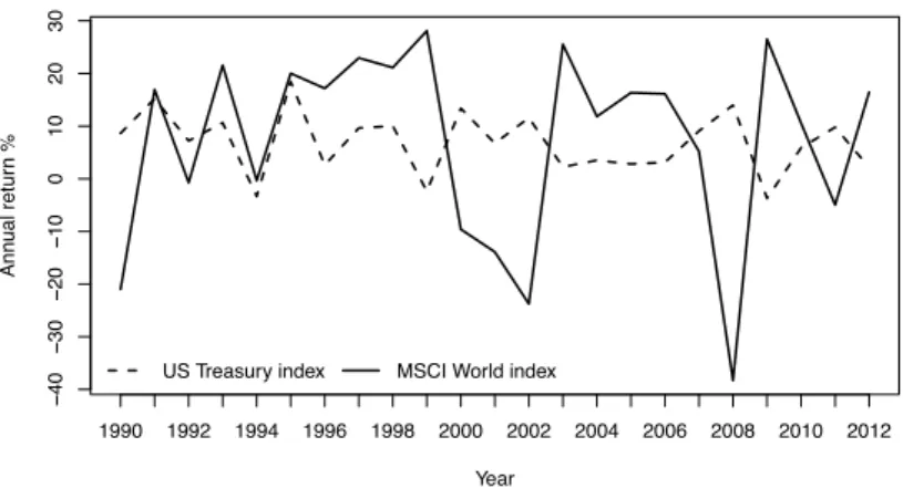
Figure 1. Annual returns for MSCI World index and US Treasury Master index
The proofs of these lower and upper probabilities are given in the Appendix, as usual in NPI these are based on counting combinations of orderings fromOA and
OB for which the event of interest must occur, to derive the lower probability (4), and for which it can occur, to derive the upper probability (5).
Based on these lower and upper probabilities, one could interpret P(ReA > e
RB + ) 0.5 as strong evidence that the future aggregate return from stock
A will exceed by at least the future aggregate return from stockB, although of course one could choose di↵erent values or include the upper probability in more detailed considerations. The results presented in this section can be extended to allow comparison of several stocks and for di↵erent events of interest, along the lines of the multiple comparisons methodology developed by Coolen and van der Laan [11] and Maturi [29].
We should emphasize that the method presented here is not explicitly aimed at optimal investment decisions or these two stocks. It will be of interest to develop the NPI approach further for such aims, for example to see how it could be applied in scenarios such as pairs trading [18, 19, 21].
4. An illustrative example
The NPI methods for future stock returns, presented in this paper, are illustrated using two real-world data sets, considering indices instead of single stocks. The first data set consists of the total returns on the MSCI World Index, which comprises 1,606 stocks from 23 developed markets across the world, providing an indication of stock market performance for global developed markets as a whole. The second data set consists of the BoA US Treasury Master index (USTre). This index measures the total return on a universe of US government bonds of all maturities, and has been chosen because it represents a comparatively less risky investment prospect than the MSCI World index. As data in this example, the annual returns on both indices spanning the period from 1990 until 2012 are used, the 23 observations for each index over this period are presented in Figure 1. The mean annual return over the period was about 7% on both indices. However, the standard deviation of MSCI World returns was about 18% while the standard deviation of US Treasury returns was about 6%. In the following illustration of the new NPI methods presented in this paper, attention is restricted to future returns over the next 3 and 6 years, of course other or more future time points could be considered.
The 23 annual returns (per index) are ordered from the smallest to the largest, and labelledr1 < . . . < r23. Appropriate values for the lower and upper bounds for the range of possible returns must be chosen, denoted by r0 and r24. The interval [r0, r24] is partitioned into 24 intervals (ri 1, ri) fori= 1, ..,24, where open intervals are used in line with the general NPI approach [6] but, for continuous data, this is of little practical relevance and one could assume half-open or closed intervals without a↵ecting the inferences. Consider future returns over the next m= 3 and
m= 6 years, this leads to 263 = 2,600 and 296 = 475,020 possible arrangements of the 3 and 6 future observations among the 23 data observations, respectively, for each index. To illustrate the use of NPI for the event that the aggregate future return over 3 and over 6 years will exceed one or more specific targets, consider target return levels ofTR= 0,1, . . . ,10%. The method presented in Section 3.1 was implemented with the statistical software R, which was used for all computations in this example. First, the NPI method described in Section 3.2 was applied in order to compare the relative levels of risk of these two indices. The NPI lower and upper probabilities were calculated for events R > Te R, for each index, for target return levelsTR= 0,1, . . . ,10%. In order to allow a fair comparison of the indices, for both data sets the lower and upper limits of the range of possible returns are set atr0 = 40% andr24= 30%.
The results of the analysis are shown in Table 1, they show several interesting features. First, imprecision (the di↵erence between corresponding upper and lower probabilities) tends to be large for the larger horizon (m= 6) than for the smaller horizon (m = 3). Typically, in NPI imprecision tends to be a decreasing func-tion of the number of available data observafunc-tions, and an increasing funcfunc-tion of the prediction horizon, this is in line with intuition. A further aspect of the NPI approach that must be emphasized, and in which it di↵ers crucially from other ap-proaches such as Monte Carlo simulation, is that them future observations which are jointly considered for inference are mutually dependent [6]. Perhaps the easiest way to think about this is that the results based on all n+m orderings of data observations and future observations being equally likely, are identical to sequen-tial application of NPI for a single observation each time, where a new observation is added to the data set before prediction of the next observation. Hence, there is more variation in the NPI approach with multiple future observations than for Monte Carlo simulation or similar approaches. Note that this increased variation is fully in line with frequentist theory as the NPI approach is exactly calibrated [27]. A more detailed study of this feature, in particular in comparison to standard bootstrap approaches and with application to a range of inferences in finance, has been initiated, we hope to report on progress in the near future.
Some aspects of the results reported in Table 1 that are worth noticing are as follows. Consider a potential investor who is interested in the events that the aggregate future return will exceed 0% (i.e. that the return will be positive), 7% (i.e. that the return will exceed the long-term average) and 10% (which would represent a strong return on this equity index). When considering the future returns over 6 years, the NPI lower and upper probabilities for exceeding an annual return of 7% and 10% in aggregate tend to be smaller than the corresponding ones over 3 years, even though this longer time horizon has led to increased imprecision. To get a positive return in m = 6 years has higher lower and upper probabilities for the MSCI than for m = 3 while for the USTRe they are quite similar when the increased imprecision is taken into account. There are several forces at play in this method of prediction, these are directly related to the observed data. For example, one or more rather extreme observed returns are likely to influence prediction more strongly for a shorter future time horizon, and also the assumed bounds r0 and
m= 3 m= 6
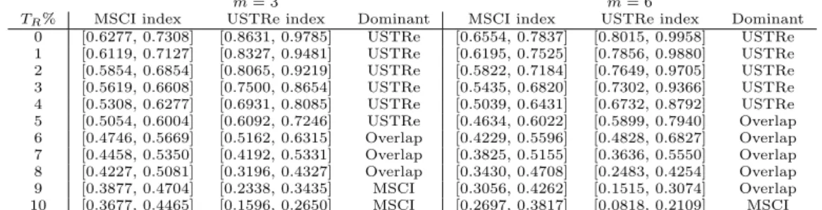
TR% MSCI index USTRe index Dominant MSCI index USTRe index Dominant
0 [0.6277, 0.7308] [0.8631, 0.9785] USTRe [0.6554, 0.7837] [0.8015, 0.9958] USTRe 1 [0.6119, 0.7127] [0.8327, 0.9481] USTRe [0.6195, 0.7525] [0.7856, 0.9880] USTRe 2 [0.5854, 0.6854] [0.8065, 0.9219] USTRe [0.5822, 0.7184] [0.7649, 0.9705] USTRe 3 [0.5619, 0.6608] [0.7500, 0.8654] USTRe [0.5435, 0.6820] [0.7302, 0.9366] USTRe 4 [0.5308, 0.6277] [0.6931, 0.8085] USTRe [0.5039, 0.6431] [0.6732, 0.8792] USTRe 5 [0.5054, 0.6004] [0.6092, 0.7246] USTRe [0.4634, 0.6022] [0.5899, 0.7940] Overlap 6 [0.4746, 0.5669] [0.5162, 0.6315] Overlap [0.4229, 0.5596] [0.4828, 0.6827] Overlap 7 [0.4458, 0.5350] [0.4192, 0.5331] Overlap [0.3825, 0.5155] [0.3636, 0.5550] Overlap 8 [0.4227, 0.5081] [0.3196, 0.4327] Overlap [0.3430, 0.4708] [0.2483, 0.4254] Overlap 9 [0.3877, 0.4704] [0.2338, 0.3435] MSCI [0.3056, 0.4262] [0.1515, 0.3074] Overlap 10 [0.3677, 0.4465] [0.1596, 0.2650] MSCI [0.2697, 0.3817] [0.0818, 0.2109] MSCI Table 1. NPI lower and upper probabilities [P , P] for the event (R > Te R)
m= 3 m= 6
Index Q1 Q3 Q3 Q1 Q1 Q3 Q3 Q1
MSCI World 4.96% 14.05% 19.01% 2.96% 10.56% 13.52% US Treasury Master 3.01% 8.81% 5.80% 2.51% 7.98% 5.47%
Table 2. Return range uncertainty measure
r24 for the range of possible returns have more influence on a shorter time period. A further force is the aforementioned dependence of the m future observations, which causes greater variability which particularly a↵ects the MSCI index as it had substantially more variability in the observed data.
Table 1 also shows, for each individual case, the results of comparison of the MSCI and USTRe indices as previously discussed, so depending on whether or not the respective intervals are overlapping. This clearly reflects that if one aims at high return, MSCI is the best investment in the sense of having substantially higher lower and upper probabilities of achieving high return. USTRe is the best option in order to achieve low but positive returns, e↵ectively because it is unlikely to lead to negative returns which are substantially more likely for MSCI. For values around the historic average of about 7% annual return, achieved by both indices over the last 23 years, the intervals are overlapping and one could not base a strong preference for either index on these data when using this specific NPI method.
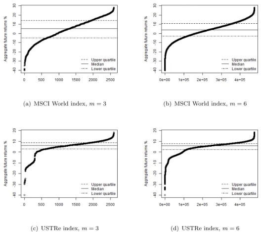
The NPI methodology for calculating an uncertainty measure based on quantiles of the range of possible values for Re, as presented in Section 3.2, leads to the results shown in Table 2, with attention restricted to the lower and upper quartiles for the lower probabilities. The return range uncertainty measure is much larger for the MSCI World index than for the US Treasury Master index, reflecting the substantially greater variability in the data for the former index and hence that the latter is less risky. This is illustrated further by the plots in Figure 2, which show the range of aggregate future lower returns, ReL, for both indices, and for
m= 3,6, as well as the lower and upper quartilesQ1 and Q3, and the median. As mentioned before, theseReLare derived by taking all possible orderings ofmfuture returns with then observed return values, and then putting each future value at the left end point of the interval that is part of the partition created by the n
observed return values. Note that particularly the tails of these distributions are quite strongly a↵ected by the choice of bounds for the range of the return values, set at r0 = 40% and r24 = 30%. The area of particular interest here, namely betweenQ1 and Q3, will be hardly a↵ected by this choice, as orderings in which one out of 3 or 6 values occur in an end interval will mostly lead to aggregate lower return outside this range. A similar plot can be made for the aggregate future upper returns, ReU, this is not presented here as the idea is similar and focus is on the lower returns, which is more interesting with a view to risk assessment and management.
An explicit way to compare two indices was presented in Section 3.3, namely by considering the event that the future aggregate return of one index will exceed,
(a) MSCI World index,m= 3 (b) MSCI World index,m= 6
(c) USTRe index,m= 3 (d) USTRe index,m= 6 Figure 2. Aggregate future lower returns valuesReL
by at least some amount , the future aggregate return of the other index. This is illustrated for the case considered in this example, again with r0 = 40% and
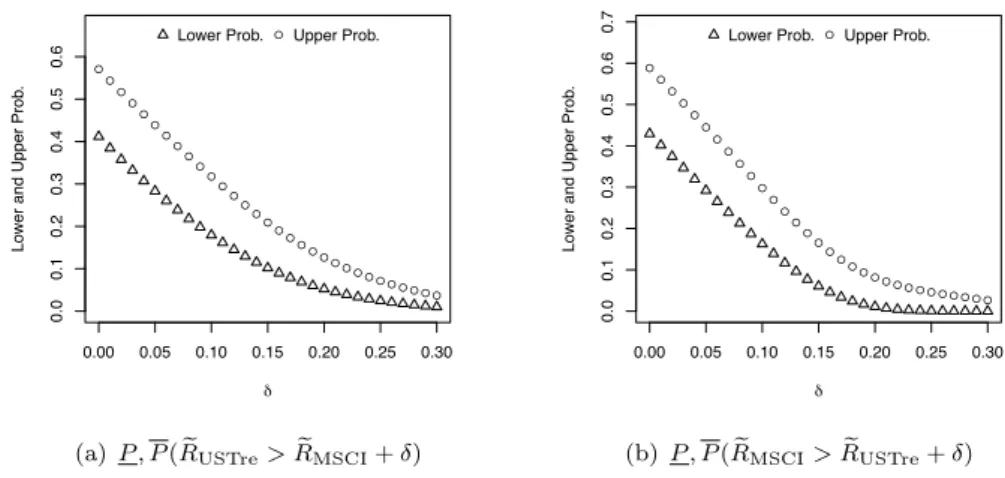
r24 = 30% for both indices and with attention restricted to future returns over the next m = 3 years. The NPI lower and upper probabilities for the event that the future aggregate return from the US Treasury index (MSCI World index) will exceed by at least = 0,1, . . . ,30% the future aggregate return from the MSCI World index (US Treasury index) are given in Figure 3(a) (Figure 3(b)). Of course, these lower and upper probabilities are decreasing as function of . The basic case of = 0 shows lower and upper probabilities which are nearly symmetric around 0.5, which is due to both indices historically having average annual returns of about 7%. The lower and upper probabilities in Figure 3(b) decrease faster than those in Figure 3(a), which is a result of the detailed orderings of the data, and hence of all future orderings per index considered; it does not necessarily reflect the greater variability of the data for the MSCI index because this variability occurs in both tails, hence there are two forces at play in such comparisons which tend to cancel each other out. These NPI lower and upper probabilities are attractive, as they address directly events of interest to an investor. The nature of these inferences is very di↵erent from established frequentist statistics methods, where for example a hypothesis of equal future returns might be tested, which gives less flexibility in focussing on the practical questions of real interest and is also harder to interpret for many people.
As mentioned before, the choice of the lower and upper limits for the range of possible return values, set at r0 = 40% and r24 = 30% for both indices in this example thus far, will have some influence on the inferences. To explore this
fur-● ● ● ● ● ● ● ● ● ● ● ● ● ● ● ● ● ●● ●● ● ● ●● ● ● ● ●● ● 0.00 0.05 0.10 0.15 0.20 0.25 0.30 0.0 0.1 0.2 0.3 0.4 0.5 0.6 δ Lo w
er and Upper Prob
.
● Lower Prob. Upper Prob.
(a)P , P(ReUSTre>ReMSCI+ )
● ● ● ● ● ● ● ● ● ● ● ● ● ● ● ● ● ●● ● ● ● ● ●● ● ● ● ●● ● 0.00 0.05 0.10 0.15 0.20 0.25 0.30 0.0 0.1 0.2 0.3 0.4 0.5 0.6 0.7 δ Lo w
er and Upper Prob
.
● Lower Prob. Upper Prob.
(b)P , P(ReMSCI>ReUSTre+ ) Figure 3. NPI lower and upper probabilities
(1) (2) (3) (4) (5) MSCI r0= 40%, r24= 30% r0= 40%, r24= 30% r0= 40%, r24= 40% r0= 50%, r24= 30% r0= 40%, r24= 30% USTre r0= 40%, r24= 30% r0= 10%, r24= 30% r0= 10%, r24= 30% r0= 10%, r24= 30% r0= 10%, r24= 20% P , P(ReMSCI>ReUSTre+ ) 0 [0.4293, 0.5882] [0.4293, 0.5631] [0.4293, 0.5695] [0.4293, 0.5631] [0.4395, 0.5631] 0.05 [0.2922, 0.4449] [0.2922, 0.4108] [0.2922, 0.4198] [0.2922, 0.4108] [0.3010, 0.4108] 0.10 [0.1625, 0.2978] [0.1625, 0.2565] [0.1625, 0.2678] [0.1625, 0.2565] [0.1675, 0.2565] 0.15 [0.0604, 0.1653] [0.0604, 0.1191] [0.0604, 0.1334] [0.0604, 0.1191] [0.0615, 0.1191] 0.20 [0.0110, 0.0815] [0.0110, 0.0347] [0.0110, 0.0480] [0.0110, 0.0347] [0.0111, 0.0347] P , P(ReUSTre>ReMSCI+ ) 0 [0.4118, 0.5707] [0.4369, 0.5707] [0.4305, 0.5707] [0.4369, 0.5708] [0.4369, 0.5605] 0.05 [0.2832, 0.4387] [0.2998, 0.4387] [0.2957, 0.4387] [0.2998, 0.4403] [0.2998, 0.4283] 0.10 [0.1794, 0.3175] [0.1889, 0.3175] [0.1865, 0.3175] [0.1889, 0.3285] [0.1889, 0.3078] 0.15 [0.1019, 0.2089] [0.1069, 0.2089] [0.1059, 0.2089] [0.1069, 0.2332] [0.1069, 0.1999] 0.20 [0.0523, 0.1265] [0.0546, 0.1265] [0.0542, 0.1265] [0.0546, 0.1523] [0.0546, 0.1187] Table 3. NPI lower and upper probabilities
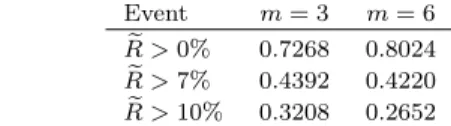
ther, the pairwise comparison method above was repeated for a variety of di↵erent choices for these limits, di↵ering for the two indices, which seems reasonable as the variabilities of the returns di↵er noticeably. Table 3 presents the results for five cases with di↵erent lower and upper limits, and only considering the values = 0,5,10,15,20%. It is clear that, for these specific inferences, hence for each specific value of and comparing the entries in the same row of the table, the choice of the limits does not have a substantial e↵ect on the NPI lower and upper probabilities. As is easily understood, the influence of these limits is also decreasing as a function of the number of available data, this follows directly from the number of intervals in the partition formed by the data, it is not illustrated in this example. To end this example, which illustrates the new theoretical methods presented in this paper, it is interesting to compare the NPI approach with Monte Carlo simu-lation, an established and indeed commonly used statistical method for predictive inferences related to stock returns. As stock market returns are often modelled by a lognormal distribution, this was assumed for the MSCI index in this example, with the two parameters estimated on the basis of the 23 observations for this in-dex. The resulting lognormal distribution was used to simulate 2,500m-year future returns. In order to compare the results with the earlier reported NPI method for this specific index, attention is restricted to predictions form= 3 andm= 6 years ahead, and the events that the aggregate future returns over the next 3 and 6 years will exceed 0,7,10%. The results from this simulation study are presented in Table 4.
The Monte Carlo simulation method gives a higher probability for achieving a positive return over the 6-year period than the 3-year period, but a smaller probability for exceeding an aggregate annual return of 10% with the longer time
Event m= 3 m= 6 e R >0% 0.7268 0.8024 e R >7% 0.4392 0.4220 e R >10% 0.3208 0.2652
Table 4. Predictive probabilities based on 2,500 Monte Carlo simulations (MSCI index)
horizon. This is likely to result from the larger impact of relatively extreme values in the simulation over the shorter period than over the longer period. The com-parison with the NPI results, as presented in Table 1, is not straightforward, as there are two main di↵erences. First, the NPI approach does not make any assump-tions about an underlying probability distribution, while the Monte Carlo method explicitly used the assumed lognormal distribution. Secondly, and this is a very important di↵erence between the two methods, the future observations in the NPI approach are dependent, which in relation to a simulation as done for the Monte Carlo method means that, if the first sampled future return value were large, it becomes slightly more likely for the next one to also be a bit larger. This leads to more variability for the future values in the NPI method than for the Monte Carlo method, however it should be emphasized that, from theoretical perspective, this greater variability is fully justified [6]. More detailed study of this e↵ect, in particular also by comparing the NPI approach to bootstrap methods, is ongo-ing, results are expected to be reported in the near future. In this example, this comparison of the results from the Monte Carlo simulation and the NPI method shows that NPI tends to lead to somewhat greater lower and upper probabilities for the events that the aggregate future return exceeds 7% and 10%, compared to the Monte Carlo probability, but mostly smaller lower and upper probabilities for the event that the aggregate future return will be positive. As mentioned, there are several aspects that influence these results, with the greater variability in the NPI method likely to be the cause for the results for the larger positive aggregate future return levels, but mostly the results from the two methods are not too far apart, with the Monte Carlo probability either inside or close to the interval created by the corresponding NPI lower and upper probabilities. One could also use this as an argument to support the assumption of a lognormal distribution as used for the Monte Carlo simulation. A similar comparison for the USTre index led to the same insights and is not reported here.
5. Concluding remarks
This paper presents the first application of NPI to aspects of finance, in particular prediction of stock returns. Of course, in order to derive at meaningful inferences about future stock returns, the underlying data set of historical stock returns must be appropriate. Key considerations include: the time period spanned by the his-torical data set to be used; the time period between observations, i.e. whether one should use daily returns, weekly returns, etc; and the values assigned to the lower and upper boundsr0 and rn+1.
The time period spanned by the data set should be considered carefully, since this has implications for the reasonableness of the exchangeability assumption discussed in Section 2. If the time period is excessively long, it may not be reasonable to assume that all past and future returns are exchangeable, since there may have been significant fluctuations in the economy or industry as a whole a↵ecting the level of stock returns. However, the data set must be large enough to provide meaningful inferences about future returns, small values of n compared to m are likely to lead to very imprecise inferences which may not be of much use.
The time period between observations is also an important consideration with regard to the exchangeability assumption. It has been proposed that certain days of the week or times of the year experience significant di↵erences with regard to stock returns and changes in market indices. These anomalies are known as calen-dar e↵ects, the most important of which are the weekend e↵ect and the January e↵ect [33]. The weekend e↵ect refers to the fact that stocks tend to exhibit rela-tively large daily returns on Fridays compared with the daily returns on Mondays. The January e↵ect refers to the larger stock returns experienced in January com-pared with those seen in other months. It may be important to account for these e↵ects when assuming exchangeability within a data set, but adaptation of the NPI method through data manipulation techniques in order to deal with such e↵ects is beyond the scope of this introductory paper. In connection to this topic, and as commented on earlier, the assumption that the original order of the historical returns is irrelevant may not be satisfactory in some real-world applications, for example if there are time series aspects beyond a general trend which are likely to have a substantial impact on the future stock returns. It may be possible to apply NPI in such cases together with some more detailed modelling, investigating this is an important topic for future research. As bootstrap methods are important for many data-based inferences in finance, it is of interest to mention the recently de-veloped NPI approach to bootstrapping [4]. This provides bootstrap samples with more variability than traditional bootstrap methods, and it will be of interest to develop it further for finance applications and to compare it to other variations such as the wild bootstrap [25].
The choice of the values r0 and rn+1 also a↵ects the inferences about future returns, this has been discussed and illustrated in the example. For the analysis undertaken in this paper, r0 was set slightly below the minimum value in the set of historical returns and rn+1 slightly above the maximum value in this set. However, detailed investigation of the impact of these values on specific inferences and in specific applications is strongly recommended, more general guidance could be achieved in future research.
The NPI methods presented in this paper provide already a relatively straight-forward approach to a variety of important topics related to future stock returns, and the frequentist statistics properties of NPI provide strong justification for the use of these methods, in particular when there is little further information about the stocks in addition to the historical data, or if one explicitly wishes not to use any additional information. There are many opportunities for extending the results in future research. It will be of interest to further investigate the impact on predic-tive probabilities of varying the timeframe and frequency of the historical returns data set, the number of future returns considered and the values assigned to the lower and upper limits on future returns. A wider range of stock selection criteria could be investigated in addition to those presented in Section 3.1 and these could be tested on a more extensive range of data sets.
Considering the dependence structure between the stock returns via copula [17, 26, 34] is another interesting research topic. A first approach to develop NPI in order to take such dependence into account has recently been published [13] and research on this topic is ongoing. NPI for multivariate data including data with additional predictors, is also an important topic for future research. Furthermore, the NPI methodology was presented for assessing the investment risk of a stock and for comparing investments with regard to their risk and uncertainty characteristics. This initial investigation into NPI-based risk measures can be extended in several ways, for example by considering di↵erent risk measures and linking it to selection of stocks for a portfolio. The application of NPI to financial analysis is a large area of
potential research to which this paper has made an important initial contribution.
Acknowledgement
The authors would like to thank three anonymous reviewers for supporting our work and for their valuable comments that helped us to improve the paper.
Appendix
The lower probability (4) is obtained by deriving the maximum lower bound for
P(ReA>ReB+ ), as follows: P(ReA>ReB+ ) = n+1m m X lB2OB P(ReA>ReB+ |RBn+j 2(rBij 1, riBj), lB 2OB, ij 2{1, . . . , n+ 1}, j= 1, . . . , m) 1 n+m m X lB2OB P(ReA>ReB+ |RBn+j =riBj, lB2OB, ij 2{1, . . . , n+ 1}, j= 1, . . . , m) = n+1m m X lB2OB P(ReA>ReBU,lB+ ) 1 n+m m 2 X lA2OA X lB2OB 1{ReAL,lA >ReBU,lB+ }=P(ReA>ReB+ )
The first (second) inequality follows by setting each future return from stock B
(stock A) in Equation (1) to be equal to the upper (lower) bound of the interval in which it falls.
The upper probability (5) is obtained by deriving the minimum upper bound for
P(ReA>ReB+ ), as follows: P(ReA>ReB+ ) = n+1m m X lB2OB P(ReA>ReB+ |RBn+j 2(rBij 1, riBj), lB 2OB, ij 2{1, . . . , n+ 1}, j= 1, . . . , m) n+1m m X lB2OB P(ReA>ReB+ |RBn+j =riBj 1, lB 2OB, ij 2{1, . . . , n+ 1}, j = 1, . . . , m) = n+1m m X lB2OB P(ReA>ReBL,lB+ ) n+1m m 2 X lA2OA X lB2OB 1{ReAU,lA >ReBL,lB+ }=P(ReA>ReB+ )
The first (second) inequality follows by setting each future return from stock B
(stock A) in Equation (1) to be equal to the lower (upper) bound of the interval in which it falls.
References
[1] Augustin, T., Coolen, F.P.A., de Cooman, G., Tro↵aes, M.C.M., 2014. Intro-duction to Imprecise Probabilities. Wiley, Chichester.
[2] Augustin, T., Coolen, F.P.A., 2004. Nonparametric predictive inference and interval probability. Journal of Statistical Planning and Inference 124, 251– 272.
[3] Baker, R.M., Coolen, F.P.A., 2010. Nonparametric predictive category se-lection for multinomial data. Journal of Statistical Theory and Practice 4, 509–526.
[4] BinHimd, S., 2014. Nonparametric Predictive Methods for Bootstrap and Test Reproducibility. PhD thesis, Durham University, www.npi-statistics.com. [5] Bodie, Z., Kane, A., Marcus, A.J., 2011. Investments and Portfolio
Manage-ment. 9 ed., McGraw-Hill, New York.
[6] Coolen, F.P.A., 2011. Nonparametric predictive inference, in: Lovric, M. (Ed.), International Encyclopedia of Statistical Science. Springer, pp. 968–970. [7] Coolen, F.P.A., 1998. Low structure imprecise predictive inference for bayes’
problem. Statistics & Probability Letters 36, 349–357.
[8] Coolen, F.P.A., 2006. On nonparametric predictive inference and objective bayesianism. Journal of Logic, Language and Information 15, 21–47.
[9] Coolen, F.P.A., Augustin, T., 2005. Learning from multinomial data: a non-parametric predictive alternative to the imprecise dirichlet model, in: Pro-ceedings of the Fourth International Symposium on Imprecise Probability: Theories and Applications, pp. 125–134.
[10] Coolen, F.P.A., Augustin, T., 2009. A nonparametric predictive alternative to the imprecise dirichlet model: the case of a known number of categories. International Journal of Approximate Reasoning 50, 217–230.
[11] Coolen, F.P.A., van der Laan, P., 2001. Imprecise predictive selection based on low structure assumptions. Journal of Statistical Planning and Inference 98, 259–277.
[12] Coolen, F.P.A., Yan, K.J., 2004. Nonparametric predictive inference with right-censored data. Journal of Statistical Planning and Inference 126, 25–54. [13] Coolen-Maturi, T., Coolen, F.P.A., Muhammad, N., 2016. Predictive inference for bivariate data: Combining nonparametric predictive inference for marginals with an estimated copula. Journal of Statistical Theory and Practice , DOI: 10.1080/15598608.2016.1184112.
[14] Coolen-Schrijner, P., Coolen, F.P.A., Shaw, S.C., 2006. Nonparametric adap-tive opportunity-based age replacement strategies. Journal of the Operational Research Society 57, 63–81.
[15] Coolen-Schrijner, P., Shaw, S.C., Coolen, F.P.A., 2009. Opportunity-based age replacement with a one-cycle criterion. Journal of the Operational Research Society 60, 1428–1438.
[16] De Finetti, B., 1974. Theory of Probability. Wiley, London.
[17] De Luca, G., Rivieccio, G., 2009. Archimedean copulae for risk measurement. Journal of Applied Statistics 36, 907-924.
[18] Do, B., Fa↵, R., 2010. Does simple pairs trading still work?. Financial Analysts Journal 66, 83-95.
[19] Do, B., Fa↵, R., 2012. Are pairs trading profits robust to trading costs?. Journal of Financial Research 35, 261-287.
[20] Ferreira, M., Santa-Clara, P., 2011. Forecasting stock market returns: the sum of the parts is more than the whole. Journal of Financial Economics 100, 514537.
[21] Gatev, E., Goetzmann, W., Rouwenhorst, K. 2006. Pairs trading: Performance of a relative-value arbitrage rule. Review of Financial Studies 19, 797-827. [22] Hampel, F., 2009. Nonadditive probabilities in statistics. Journal of Statistical
Theory and Practice 3, 11–23.
[23] Henkel, S., Martin, J., Nadari, F., 2011. Time-varying short-horizon pre-dictability. Journal of Financial Economics 99, 560580.
[24] Hill, B.M., 1968. Posterior distribution of percentiles: Bayes’ theorem for sampling from a population. Journal of the American Statistical Association 63, 677–691.
[25] Kim, J., 2006. Wild bootstrapping variance ratio tests. Economics Letters 92, 38-43.
[26] Krupskii, P.,Joe, H., 2015. Tail-weighted measures of dependence. Journal of Applied Statistics 42, 614-629.
[27] Lawless, J.F., Fredette, M., 2005. Frequentist prediction intervals and predic-tive distributions. Biometrika 92, 529–542.
[28] Ludvigson, S., Ng, S., 2007. The empirical risk-return relation: a factor anal-ysis approach. Journal of Financial Economics 83, 171222.
[29] Maturi, T.A., 2010. Nonparametric Predictive Inference for Multiple Com-parisons. PhD thesis, Durham University, www.npi-statistics.com.
[30] Pesaran, M.H., Timmermann, A., 1995. Predictability of stock returns: Ro-bustness and economic significance. The Journal of Finance 50, 1201–1228. [31] Rapach, D., Strauss, J., Zhou, G., 2010. Out-of-sample equity premium
predic-tion: combination forecasts and links to the real economy. Review of Financial Studies 23, 821-862.
[32] Rapach, D., Zhou, G., 2013. Chapter 6 - forecasting stock returns, in: Elliott, G., Timmermann, A. (Eds.), Handbook of Economic Forecasting. Elsevier. volume 2, Part A ofHandbook of Economic Forecasting, pp. 328 – 383. [33] Sullivan, R., Timmermann, A., White, H., 2001. Dangers of data mining: the
case of calendar e↵ects in stock returns. Journal of Econometrics 105, 249–286. [34] Trede, M., Savu, C., 2013. Do stock returns have an Archimedean copula?.
Journal of Applied Statistics 40, 1764-1778.
[35] Wilmott, P., 2007. Paul Wilmott introduces quantitative finance. 2 ed., Wiley, Chichester.