Monetary-Fiscal Policy
Interactions and Fiscal
Stimulus
Troy Davig and Eric M. Leeper
November 2009
Monetary-Fiscal Policy Interactions
and Fiscal Stimulus
Troy Davig and Eric M. Leeper November 2009
RWP 09-12
Abstract
Increases in government spending trigger substitution effects—both inter- and intra-temporal—and a wealth effect. The ultimate impacts on the economy hinge on current and expected monetary and fiscal policy behavior. Studies that impose active monetary policy and passive fiscal policy typically find that government consumption crowds out private consumption: higher future taxes create a strong negative wealth effect, while the active monetary response increases the real interest rate. This paper estimates Markov-switching policy rules for the United States and finds that monetary and fiscal policies fluctuate between active and passive behavior. When the estimated joint policy process is imposed on a conventional new Keynesian model, government spending generates positive consumption multipliers in some policy regimes and in simulated data in which all policy regimes are realized. The paper reports the model’s predictions of the macroeconomic impacts of the American Recovery and Reinvestment Act’s implied path for government spending under alternative monetary-fiscal policy combinations.
JEL Nos.: E31, E52, E6, E62
Keywords: fiscal policy, government multiplier, monetary-fiscal interactions
Date: July 14, 2009. We thank Ignazio Angeloni, Dale Henderson, Jim Nason, and seminar participants at the Konstanz Seminar, Sveriges Riksbank, and the conference on “Monetary-Fiscal Policy Interactions, Expectations, and Dynamics in the Current Economic Crisis” at Princeton University for comments. Research Department, Federal Reserve Bank of Kansas City, troy.davig@kc.frb.org; Department of Economics, Indiana University and NBER, eleeper@indiana.edu. The views expressed herein are those of the authors and do not necessarily represent those of the Federal Reserve Bank of Kansas City or the Federal Reserve System.
Monetary and fiscal policy responses to the recession of 2007-09 have been un-usually aggressive, particularly in the United States. The Federal Reserve rapidly reduced the federal funds rate more than 500 basis points, beginning in the summer of 2007, and the rate has effectively been at its zero bound since December 2008. Early in 2009 the U.S. Congress passed the $787 billion American Recovery and Reinvestment Act, in addition to the $125 billion provided by the Economic Stimu-lus Act of 2008. The Congressional Budget Office (2009) projects that the Federal deficit will be 13 percent of GDP in 2009 and, with the passage of President Obama’s budget, deficits will hover around 5 percent of GDP through 2019; as a consequence, government debt as a share of GDP is expected to rise from 40 percent in 2008 to 80 percent in 2019. With the exception of wars and the Great Depression, the projected speed of debt accumulation is unprecedented in the United States. This unified and aggressive monetary-fiscal front to stimulate the economy is a distinctive feature of the current policy response.
The overriding objective of the stimulus efforts is to spur job creation by increasing aggregate demand, particularly in the short run [Romer and Bernstein (2009), Board of Governors of the Federal Reserve System (2008)]. Because private consumption constitutes about two-thirds of GDP, the typical argument has stimulus raise con-sumption demand, the demand for labor, and employment. It is ironic that the consumption response to an increase in government spending is the linchpin in the transmission mechanism for fiscal stimulus: economic theory and empirical evidence do not universally support the idea that higher government purchases raise private consumption.
Two features of the macro policy response have received little modeling attention, despite being central to the predictions of the impacts of the policy actions. First, monetary and fiscal policy have reacted jointly in an effort to stimulate aggregate demand. A long line of research emphasizes that separating monetary and fiscal poli-cies overlooks policy interactions that are important for determining equilibrium.1
Second, few economic observers expect that the current recession-fighting mix of macro policies will persist indefinitely; eventually, policies will return to “normal.” Because the impacts of current policies depend, in part, on expectations of possible
1
Examples include Sargent and Wallace (1981), Wallace (1981), Aiyagari and Gertler (1985), Sims (1988), and Leeper (1991).
future monetary-fiscal policy regimes, predictions need to condition on the current regime and incorporate prospective future regimes.2
Intertemporal aspects of mone-tary and fiscal policy interactions determine how any fiscal stimulus is expected to be financed, which theory suggests is a critical determinant of the efficacy of the stimulus.
This paper addresses these two features in a conventional dynamic stochastic gen-eral equilibrium (DSGE) model with nominal price rigidities and complete specifica-tions of monetary and fiscal policies. The model embeds the possibility that policy rules may evolve over time according to a known probability distribution and that private agents form expectations of policy according to that distribution. We esti-mate simple interest rate and tax policy rules whose parameters are governed by a Markov chain. The estimated joint monetary-fiscal policy process is inserted into the calibrated DSGE model. Government spending, which is a central focus of the analysis, evolves exogenously.
In this setting, an increase in unproductive government spending sets in motion both intra- and inter-temporal substitution effects, as well as a wealth effect.3,4
Rel-ative sizes of these effects determine how real wages, employment, consumption, and inflation react. Typical analyses assume passive fiscal behavior, which couples higher government spending with an equivalent increase in lump-sum taxes to pay for the spending, while the analyses also assume active monetary policy [see, for example, Gali, Lopez-Salido, and Valles (2007), Ravn, Schmitt-Grohe, and Uribe (2007), and Monacelli and Perotti (2008)].5 Under this set of policies, the intra-temporal sub-stitution effect is triggered when higher government spending increases aggregate demand and, because output is demand-determined, raises the demand for labor. As
2
Work along these lines is more limited, but includes Leeper and Zha (2003), Davig and Leeper (2006), Chung, Davig, and Leeper (2007), and Davig and Leeper (2007), Svensson and Williams (2007, 2008), Bianchi (2009), and Farmer, Zha, and Waggoner (2009).
3
We use the term “unproductive” government spending to refer to those government purchases of goods and services that do not directly enhance the production possibilities or productivity of private firms.
4Monacelli and Perotti (2008) nicely explain how these mechanisms operate under flexible and
sticky prices and under the two sets of preference specifications due to King, Plosser, and Rebelo (1988) and Greenwood, Hercowitz, and Huffman (1988).
5Monetary policy is passive when the central bank raises the nominal interest rate only weakly
in response to inflation and fiscal policy is active when taxes and spending do not adjust in order to stabilize government debt [Leeper (1991)].
the real wage rises, households work harder, substituting consumption for leisure. An increase in the real wage is necessary for government spending to have a positive effect on private consumption. Higher real wages increase firms’ marginal costs and cause them to raise prices, if given the opportunity under the Calvo (1983) pricing mechanism.
Inter-temporal effects work through the real interest rate, whose movements de-pend on how monetary policy responds to changes in inflation arising from changes in government purchases. When prices are sticky, an increase in government pur-chases gradually raises the price level, thereby raising the expected path of inflation. An active monetary response raises the nominal interest rate sharply, which raises the real rate and induces agents to postpone consumption. Higher taxes create a negative wealth effect that shifts out the supply of labor—when leisure is a normal good—further increasing hours worked, but offsetting at least some of the increase in real wage. Most importantly, because consumption is also a normal good, higher taxes induce households to shift down their consumption paths, ultimately reducing equilibrium consumption, as Barro and King (1984) and Baxter and King (1993) show.
Changes in government spending are most often studied in a regime with active monetary and passive fiscal policy. One exception is Kim (2003), who follows up on the analysis in Woodford (1998) to show that under alternative assumptions about the monetary-fiscal regime—specifically, passive monetary policy and active fiscal policy—higher government spending consistently raises both output and consump-tion. Under that alternative mix of policies, higher government spending also creates higher expected inflation. Instead of raising the real rate, passive monetary policy does not increase nominal rates strongly with inflation, so the real rate declines. The lower real rate reduces the return to saving and induces agents to increase current consumption demand. Active fiscal policy means that higher taxes are not expected to fully finance the increase in government spending, and the usual negative wealth effect on labor supply and consumption is mitigated, even with standard preferences such as those introduced by King, Plosser, and Rebelo (1988).
These substitution and wealth effects operate in the model with regime-switching policies, but their relative sizes vary across regimes. We explain these mechanisms using two viewpoints. The first is from the perspective of the firms’ and households’ optimal decisions, as explained above. A second viewpoint utilizes the intertemporal
equilibrium condition that equates the real value of nominal government liabilities to the expected present value of future net-of-interest surpluses inclusive of seigniorage revenues.6 From this standpoint, a higher expected path of government spending, with no associated higher path of taxes, reduces the fiscal backing for government liabilities, driving down their value.7 Households convert government debt into con-sumption, reinforcing the initial increase in aggregate demand. The value of debt in terms of goods must fall, so the price level must rise. Regime-switching policies imply that this debt revaluation mechanism is always in play, but its importance is a quantitative matter, depending on the relative probabilities of various regimes.
This paper reports quantitative results. Government spending multipliers for output—computed as the present value of the change in output as a ratio of the present value of the change in government spending—vary from a bit below 1 to near 2, depending on the monetary-fiscal regime that is assumed to prevail. The as-sociated multipliers for consumption may be negative or close to one, depending on the policy regime. VARs estimated from simulated data in which policies fluctuate among all four possible combinations—one active and one passive; both passive; both active—yield mean government spending impact multipliers that peak for output at about 1.7 and for consumption at about 0.7, close to estimates from the fiscal VAR literature.
The model in this paper assumes a fixed capital stock, which shuts off the possible channel that would allow consumption to rise by crowding out investment. Thus, our quantitative estimates are conservative relative to models that exploit this channel to raise the consumption multiplier.
The channels through which government spending affects prices and quantities in this paper seem highly plausible. They rely only on the observation that monetary-fiscal regimes have changed and are expected to continue to change over time, fluc-tuating between active and passive periods. Otherwise, the environment we study is completely conventional. Existing methods for generating positive government spending multipliers for consumption do not conflict, and likely would amplify, the channels that this work highlights.
6Leeper and Yun (2006) develop a Slutsky-Hicks decomposition to systematically study these
effects in the context of changes in distorting taxes.
7Cochrane (2005, p. 502) refers to this intertemporal equilibrium condition as a “valuation
With the calibrated model in hand, we simulate the impacts of the government spending component of the American Recovery and Reinvestment Act of 2009 un-der alternative monetary-fiscal regimes. When monetary policy is active and fiscal policy is passive, the fiscal stimulus creates a modest expansion in output and it raises inflation and real interest rates, while government debt and taxes rise substan-tially and persistently. On the other hand, passive monetary policy and active fiscal policy generate an appreciably larger boom in output and consumption, and a signif-icantly larger run-up in inflation, while rapidly reducing the real value of government liabilities.
The paper concludes by considering the probable scenario that, as inflation rises due to the fiscal stimulus, the Federal Reserve combats inflation by switching to an active stance, but fiscal policy continues to be active. Of course, doubly active policies, if they were expected to persist indefinitely, would imply that no equilibrium exists. With Markov switching, however, the economy can visit such a regime because individuals expect the visit to be temporary. In this scenario, output, consumption, and inflation are chronically higher, while debt explodes and real interest rates decline dramatically and persistently.
Taken together, the paper’s results argue forcefully that the impacts of a fiscal stimulus cannot be understood without studying monetary and fiscal policies jointly. Moreover, different assumptions about joint monetary-fiscal behavior can lead to sharply different conclusions about the likely consequences of fiscal stimulus.
2. Selective Review of Work on Government Spending
In recent years, a small industry of research has sprung up to reconcile the theoreti-cal and empiritheoreti-cal findings about the impacts of increases in unproductive government spending on private consumption. As initially pointed out by Barro and King (1984) and Baxter and King (1993), neo-classical theory predicts that higher government consumption that is financed by lump-sum taxes reduces household wealth and, therefore, the path of private consumption. In contrast, a range of empirical studies finds that government consumption crowds in private consumption [Blanchard and Perotti (2002), Perotti (2007), Ravn, Schmitt-Grohe, and Uribe (2007), Mountford
and Uhlig (2009)].8 Using U.S. data, Gali, Lopez-Salido, and Valles (2007) estimate the government spending multiplier for output to be 0.80 initially and rising to 1.74 after two years, while the multiplier for consumption is always positive and is 0.17 on impact and 0.95 after two years. Monacelli and Perotti (2008) report similar results across several empirical specifications.
A variety of theoretical channels have been suggested to ensure that the negative wealth effect on consumption does not overwhelm the substitution effect. Many suggestions amount to changing the representative household’s preferences. Ravn, Schmitt-Grohe, and Uribe (2007), for example, assume deep habits that amplify the increase in real wages and, therefore, the size of the substitution effect. Monacelli and Perotti (2008) eliminate the wealth effect on labor supply, which generates strong complementarity between consumption and work effort.9
Gali, Lopez-Salido, and Valles (2007) is a departure from efforts to intervene on preferences, but the alternative is rather complex. Heterogenous agents—some fully optimizing and others operating by rules of thumb—are combined with imperfectly competitive labor markets—labor unions set wages—in a new Keynesian model with sticky prices to produce positive government spending multipliers for consumption.
This paper combines an off-the-shelf new Keynesian model—described in the next section—with estimated regime-switching monetary and fiscal policies to explore more thoroughly the channel that Kim (2003) points to by which government spend-ing can have multiplied impacts on output and, therefore, produce positive multipli-ers for consumption.
3. A New Keynesian Model with Variable Government Purchases
The analysis is conducted in a conventional new Keynesian model with fixed capi-tal and elastic labor supply. Nominal rigidities are introduced through Calvo (1983)
8Not all empirical work supports the crowding in view. Ramey and Shapiro (1998) and Ramey
(2007), for example, argue that anticipated increases in government spending reduce private consumption.
9Bouakez and Rebei (2007) intervene on preferences by assuming private consumption and
pub-lic goods are complements. Linnemann (2006) obtains positive government spending multipliers for consumption in a frictionless real business cycle model by assuming particular non-separable preferences over consumption and leisure, but Bilbiie (2008) shows that Linnemann’s preferences imply both a downward sloping labor supply function and that consumption is an inferior good.
pricing by monopolistically competitive final goods producing firms. Unproductive government spending is financed through a combination of lump-sum taxes, seignior-age revenues, and one-period nominal government bonds.
3.1. Households. The representative household chooses {Ct, Nt, Mt, Bt} to
maxi-mize Et ∞ X i=0 βi " C1−σ t+i 1−σ −χ Nt1++iη 1 +η +δ (Mt+i/Pt+i)1−κ 1−κ # (1) with 0 < β < 1, σ > 0, η > 0, κ > 0, χ > 0 and δ > 0, where Ct is a composite
consumption good consisting of differentiated goods, cjt,which are aggregated using
the Dixit and Stiglitz (1977) aggregator
Ct= Z 1 0 c θ−1 θ jt dj θ θ−1 , θ > 1. (2) The household chooses each good cjt to minimize total expenditure, yielding the
demand functions for each good j cjt = pjt Pt −θ Ct, (3) wherePt ≡ hR1 0 p 1−θ jt dj i 1 1−θ .
The household’s budget constraint is
Ct+ Mt Pt + Bt Pt +τt ≤ Wt Pt Nt+ Mt−1 Pt +(1 +rt−1)Bt−1 Pt + Πt, (4)
whereτtis lump-sum taxes/transfers,Btis one-period nominal bond holdings, 1+rt−1
is the risk-free nominal interest rate betweent−1 and t, and Πt is profits from the
firm. The household maximizes (1) subject to (4), yielding
χ N η t C−σ t = Wt Pt (5) 1 =β(1 +rt) Ct Ct+1 σ Pt Pt+1 . (6)
resulting in the following relation between real money balances, the nominal rate and the composite consumption good,
Mt Pt =δκ rt 1 +rt −1/κ Ctσ/κ. (7)
The government’s demand for goods is in the same proportion as households, yielding the government’s demand as gjt =
pjt Pt −θ Gt, whereGt = hR1 0 g θ−1 θ jt dj i θ θ−1 .
Necessary and sufficient conditions for household optimization require (5)-(7) to hold in every period and the household’s budget constraints to bind with equality. In addition, the present value of households’ expected expenditures are bounded and the following transversality condition holds
lim T→∞ Et qt,T AT PT = 0, (8) whereAt=Bt+Mt and qt,T = (1 +rT−1)/(PT/Pt).
3.2. Firms. A continuum of monopolistically competitive firms produce goods using labor. Production of good j is
yjt =ZNjt, (9)
whereZ is aggregate technology, common across firms and taken to be constant. Aggregating consumers’ and government’s demand, firmj faces the demand curve
yjt = pjt Pt −θ Yt, (10) whereYt is defined by Ct+Gt=Yt. (11)
Equating supply and demand for individual goods,
ZNjt = pjt Pt −θ Yt. (12)
Following Calvo (1983), a fraction 1−ϕ firms are permitted to adjust their prices each period, while the fractionϕ are not permitted to adjust. If firms are permitted
to adjust prices at t, they choose a new optimal price, p∗
t,to maximize the expected
discounted sum of profits given by
Et ∞ X i=0 ϕiqt,t+i " p∗ t Pt+i 1−θ −Ψt+i p∗ t Pt+i −θ# Yt+i, (13)
where the real profit flow of firm j at period t, Πjt =
pjt
Pt
1−θ
Yt−WPttNjt, has been
rewritten using (12). Ψt is real marginal cost, defined as
Ψt=
Wt
ZPt
. (14)
The first-order condition that determinesp∗
t can be written as p∗ t Pt = θ θ−1 EtP∞ i=0(ϕβ)i(Yt+i−Gt+i) −σ Pt+i Pt θ Ψt+iYt+i Et P∞ i=0(ϕβ)i(Yt+i−Gt+i)−σ Pt+i Pt θ−1 Yt+i , (15) which we denote by p∗ t Pt = θ θ−1 K1t K2t , (16)
where the numerator and the denominator have recursive representations:
K1t= (Yt−Gt) −σ ΨtYt+ϕβEtK1t+1 Pt+1 Pt θ (17) and K2t= (Yt−Gt) −σ Yt+ϕβEtK2t+1 Pt+1 Pt θ−1 . (18) Solving (16) for p∗
t and using the result in the aggregate price index, P1
−θ t = (1−ϕ)(p∗ t)1 −θ +ϕP1−θ t−1, yields πθ−1 t = 1 ϕ − 1−ϕ ϕ µK1t K2t 1−θ , (19) whereµ≡θ/(θ−1) is the markup.
We assume that individual labor services may be aggregated linearly to produce aggregate labor, Nt =
R1
conditions implies ZNt = ∆tYt, where ∆t is a measure of relative price dispersion defined by ∆t = Z 1 0 pjt Pt −θ dj. (20) Now the aggregate production function is given by
Yt=
Z
∆t
Nt. (21)
It is natural to define aggregate profits as the sum of individual firm profits, Πt =
R1
0 Πjtdj. Integrating over firms’ profits and combining the household’s and the government’s budget constraints yields the aggregate resource constraint
Z
∆t
Nt=Ct+Gt. (22)
From the definitions of price dispersion and the aggregate price index, relative price dispersion evolves according to
∆t= (1−ϕ) p∗ t Pt −θ +ϕπtθ∆t−1, (23) whereπt =Pt/Pt−1.
Following Woodford (2003), we define potential, or the natural level of, output,Ytp,
to be the equilibrium level of output that would be realized if prices were perfectly flexible. Potential output, then, emerges from the model whenϕ= 0, so all firms can adjust prices every period. In the current setup, potential would vary systematically with government spending, but not with monetary policy or lump-sum tax shocks. In the empirical work, we use the Congressional Budget Office’s measure of potential GDP, which is essentially a smooth trend for output, YT
t ; it certainly does not
coincide with the theoretical concept of the natural level of output. To make our theory line up with the empirical work, we define the output gap,yt, as yt=Yt−YtT,
with YT
t ≡1 for all t, since we abstract from growth.
4. Policy Specification
4.1. Regime-Switching Policy Rules. To account for possible changes in regime, the policy rules take the same form as in Davig and Leeper (2006). Specifically, the
monetary policy rule is
rt =α0(StM) +απ(StM)πt+αy(StM)yt+σr(StM)εrt, (24)
whereπt is inflation,yt is the output gap, and εrt ∼i.i.d. N(0,1) is the disturbance.
SM
t indicates the monetary policy regime and follows a four-state Markov chain. The
variance of the errors switches between two different values independently of the coefficients in the rule. Since coefficients may take two different regime-dependent values as well, there are a total of four monetary regimes. Estimates are given in table 1 and filtered and smoothed probabilities are given in figure 1. The sample runs from 1949:Q1 to 2008:Q4. The rule also includes a dummy to account for the credit controls in place in the early 1980s; however, its estimated value is insignificant.
The fiscal rule also takes the same form as in Davig and Leeper (2006). All parameters are restricted to switch simultaneously, so a change in behavior, say in the response of taxes to the output gap, imposes a change in the responses to debt and government purchases. The fiscal rule is
τt =γ0(StF) +γb(StF)bt−1+γy(S
F
t )yt+γg(StF)gt+στ(StF)ετt, (25)
whereτtis the ratio of lump-sum taxes—defined as government revenues less transfers—
to output, bt−1 is lagged debt-to-output ratio, gt is the government
purchase-to-output ratio and ετ
t ∼ N(0,1). StF indicates the fiscal policy regime, which follows
a Markov chain with transition matrix PF. The fiscal rule also allows the variance
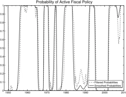
of the errors to switch between two values, but the changes are restricted to occur simultaneously with changes in the coefficients. Consequently, there are two fiscal regimes. The sample ends one quarter earlier than the sample for estimating the monetary rule due to data availability. Estimates are given in table 2 and filtered and smoothed probabilities are in figure 2.
When embedding the rules into the new Keynesian model, we aggregate the four monetary states into two states that differ across reaction coefficients.10 This has no impact on the numerical solution in the next section because, although we estimate the policy rules allowing for random disturbances, we turn off the random shocks to
10The aggregation sums transition probabilities across volatility regimes, then weights each sum
so that the percentage of time spent in the active monetary policy regime is the same in the two-state chain as in the four-state chain. For example, based on the definition of monetary
regimes given in table 1, then Pr[St = 1|St−1 = 1] ≡ Pr[S
M t = 1]/Pr[S M t = 1] + Pr[S M t = 2] + Pr[SM t = 2]/Pr[S M t = 1] + Pr[S M t = 2]
, where St is the aggregated regime, S
M
t = 1 is the
low-volatility active regime andSM
taxes and monetary policy when solving the model. The only random disturbance we consider is to government purchases.
The aggregated transition matrix for monetary policy and estimated transition matrix for fiscal policy are as follows
PM = .97 .03 .01 .99 , PF = .94 .06 .05 .95 . (26)
The joint transition matrix governing the monetary-fiscal regime is then P =
PM ⊗PF. Figure 3 illustrates the estimated timing of the monetary-fiscal regime.
Throughout the first half of the sample, monetary policy was passive, consis-tent with estimates of Taylor rules [Clarida, Gali, and Gertler (1999) or Lubik and Schorfheide (2004)]. Fiscal policy, however, switched between active and passive regimes. Monetary studies that maintain the assumption that fiscal policy is perpet-ually passive would conclude that the rational expectations equilibrium is indetermi-nate, as Lubik and Schorfheide (2004) argue. The early to mid-1980s was a period in which both policies were active, a policy mix that would imply non-existence of equilibrium if it were expected to persist indefinitely. This was also a time when economic commentators described U.S. fiscal policy as unsustainable because govern-ment debt was growing rapidly as a share of GDP. While monetary policy remained active through the 1980s, first under Federal Reserve Chairman Paul Volcker and then Chariman Alan Greenspan, fiscal policy adopted a passive stance as many of the Reagan tax cuts were reversed. The recessions of 1990-91 and 2000-01 induced monetary policy to switch to being passive, while the tax cuts of George W. Bush are reflected as an active fiscal stance through the 2000s. The joint policy process throughout much of the 2000s has been passive monetary policy and active fiscal policy. Evidently, there is substantial instability in fiscal policy, but greater stability in monetary policy behavior, an outcome also found by Favero and Monacelli (2005).
Government purchases evolve according to log (Gt) = log G
(1−ρ) +ρlog (Gt−1) +εt, (27)
4.2. The Government’s Flow Budget Identity. The processes for{Gt, τt, Mt, Bt}
must satisfy the flow government budget identity
Gt=τt+ Mt−Mt−1 Pt +Bt Pt −(1 +rt−1)Bt−1 Pt . (28) given M−1 >0 and (1 +r−1)B−1.
4.3. Steady-State Values. Steady-state debt levels conditional on the AM/PF, PF/PF and PM/AF regimes are set to be equal across regimes. Mechanically, this is done by substituting the tax rule into the budget constraint and setting output to its deterministic steady state level of unity, then solving for the intercept in the tax policy rule. These calculations yield
γ0 StF =G−m π 1 +π −b 1 +γ StF− β −1 (1 +π) , (29) where each variable, except γ0 StF
and γ SF t
is set to its steady-state value. An analogous procedure is performed on the monetary policy rule, (24), and the money demand relation, (7). As with debt, steady-state rates of inflation are set to be equal across the AM/PF, PF/PF and PM/AF regimes.
For the AM/AF regime, steady-state debt is not a well defined concept, since real debt follows a nonstationary path. In this regime, an innovation to the level of debt does not elicit a sufficient response from future taxes to stabilize the path of debt. However, the active-active regime is not expected to last indefinitely, as the transversality condition on debt is satisfied via an expectation of a switch to a future policy regime.
5. Solution and Calibration
We set the parameters governing preferences, technology and price adjustment to be consistent with Rotemberg and Woodford (1997) and Woodford (2003). The model is calibrated at a quarterly frequency. Firms markup the prices of their goods over marginal cost by 15 percent, implyingµ=θ(1−θ)−1
= 1.15, and 66 percent of firms cannot reset their price each period (ϕ=.66). The quarterly real interest rate is set to 1 percent (β =.99). Preferences over consumption are logarithmic, soσ = 1. We also set the Frisch labor supply elasticity to unity, soη= 1 and setχso the steady state share of time spent in employment is 0.2. Intermediate goods-producing firms utilize a constant-returns-to-scale production function. The technology parameter,
Z, is set to normalize the deterministic steady state level of output to unity. Steady state inflation is set to 2 percent and the steady state debt-output ratio is set to .35. For real balances, we setδso velocity in the deterministic steady state, defined as
cP/M, corresponds to the average U.S. monetary base velocity at 2.4. We take this value from Davig and Leeper (2006), where we computed it using data from 1959-2004 on the average real level of expenditure on non-durable consumption plus services. The parameter that determines the interest elasticity of real money balances,κ, is set to 2.6 [Mankiw and Summers (1986), Lucas (1988), Chari, Kehoe, and McGrattan (2000)].
Coefficients in the monetary and fiscal rules are set to their estimated values with one exception: the coefficient on government purchases in the fiscal rule is set to zero. The actual estimates for these coefficients are positive and imply that taxes begin rising in the same period as the increase in government purchases. Ruling out the immediate tax response to government purchases better isolates the impact of government purchases. Taxes continue to respond, however, to the movements in debt and output generated by the change in government purchases.
To obtain parameter values in the process for government purchases, we estimate
ρ and σ2 in (27) by detrending the log of real total government purchases from 1949:Q1-2009:Q1. Estimation yields a value forρ of .9 and the value of σ2 implies a one-standard deviation shock raises the level of government purchases 1.5%. Steady state purchases, G, is set so purchases equal 20% of output in the deterministic steady state.
We solve the model numerically using the monotone map method described in Davig and Leeper (2006).
6. Dynamic Impacts of Government Purchases
In the new Keynesian framework, the general mechanisms through which a change in government purchases affects the equilibrium, regardless of the monetary-fiscal regime, are:
• higher government spending raises demand for the goods sold by monopolis-tically competitive intermediate-goods producing firms;
• intermediate-goods producing firms meet demand at posted prices by increas-ing their demand for labor;
• higher labor demand raises real wages and real marginal costs;
• firms that have the option of reevaluating their pricing decision will increase their prices.
These mechanisms operate across each monetary-fiscal regime. Also, the positive comovement of output and prices occurs in each regime, so an unproductive govern-ment spending shock looks like a traditional “demand” shock regardless of policy. The policy regime, however, does play a critical role in determining the movement of real rates, consumption and the path for inflation.
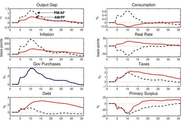
To highlight the differences and similarities across regimes, figure 4 reports the im-pulse responses to a two-standard deviation shock to government purchases, which translates to a 3 percent rise in the level of purchases, conditional on each of the three stationary regimes. The experiment holds regime fixed, although agents’ ex-pectations functions embed the probability that regimes can change. In each regime, output rises as government purchases increase demand, causing firms to hire more labor and increase production. Households experience a rise in their real wage due to the increase in demand for their labor services (i.e., they slide along their labor supply curve), but also realize some decline in wealth arising from higher expected tax payments. From the monopolistic firms’ perspective, the rise in the real wage drives up their real marginal costs. Since government purchases are serially corre-lated, the rise in marginal costs is expected to be persistent; if given the opportunity under the Calvo pricing restrictions, an individual firm will respond to the shock by raising its price.
Under active monetary and passive fiscal policy, which is the benchmark policy configuration in many studies and exhibits Ricardian equivalence in the fixed-regime setting, the monetary authority responds aggressively to the rise in inflation by in-creasing the nominal rate more than one-for-one (dashed lines). As figure 4 indicates, the monetary response persistently raises the real rate and dampens consumption demand from households. As purchases return to their steady state level, the real rate falls and consumption rises back to steady state. Since inflation remains rela-tively subdued, seigniorage revenues play a small role in governing debt dynamics. Taxes respond to lagged debt and rise as the government issues debt to finance the expanded level of purchases. However, taxes do not respond sufficiently to result
in monotonically declining debt, so debt peaks roughly 10 periods after the initial shock.
The dynamics of output and consumption in the active monetary/passive fiscal (AM/PF) regime qualitatively resemble those of a standard real-business cycle model, where an increase in government purchases acts as a negative shock to lifetime wealth, which causes agents to decrease both consumption and leisure. The rise in time spent working stimulates output, but not enough to cause consumption to rise. The drop in consumption, both in the AM/PF regime and real business cycle model stands in contrast to traditional Keynesian policy analysis. Textbook formulations posit that an increase in government purchases generates dynamics—sometimes referred to as “Keynesian hydraulics”—that produce a multiple increase in output and consump-tion, where the multiple depends on the marginal propensity to consume [Branson (1989)].
As discussed in the introduction, mechanisms that cause consumption to rise in modern general equilibrium settings often require modifying preferences or introduc-ing incomplete markets and labor market imperfections. An alternative to these modifications is to assume a different policy regime with passive monetary and ac-tive fiscal policy. Kim (2003) shows in a fixed-regime new Keynesian model that an increase in government purchases can increase consumption under passive mon-etary/active fiscal (PM/AF) policy by inducing the real rate to decline. Figure 4 demonstrates that the same mechanism exists in the regime-switching framework (light solid lines). The increase in government purchases, which is expected to be persistent, raises current and future demand, so raises inflation expectations. Under passive monetary policy, the monetary authority responds to the increase in inflation less than one-for-one and lets the real rate fall. The lower future path of the real rate lowers the return to saving, which stimulates demand as households pull consump-tion forward. This model holds the capital stock fixed and is a closed economy, so the increase in government purchases and consumption generates an output multiplier greater than one and a larger increase in output than under AM/PF policy. The large increase in output above potential generates a substantially larger increase in inflation than in the AM/PF regime.
The larger response of output under passive monetary policy also raises taxes by more on impact than under active monetary policy, since the tax rule specifies taxes rise in response to the output gap. Under passive monetary/passive fiscal (PM/PF)
policy, the response of taxes to output is larger than in PM/AF, so taxes increase relatively more and debt rises by less on impact.
To better understand the debt dynamics, recall that following intertemporal equi-librium condition must hold in every regime
Mt−1 + (1 +rt−1)Bt−1 Pt =Et ∞ X T=t qt,T τT −GT + rT 1 +rT MT PT , (30) which indicates that the present value of primary surpluses and seigniorage must equal the real value of outstanding nominal government liabilities. Holding every-thing constant except government purchases, equilibrium condition (30) implies that an increase in government purchases, financed by new debt issuance, lowers the present value of primary surpluses and creates an imbalance between the initial value of liabilities and their expected backing (i.e., the right-hand side variables).
To restore balance, a number of adjustments can occur. First, the present value of taxes may rise by exactly the amount that government purchases changed, which is the adjustment that occurs under a Ricardian regime. Second, the present value of seigniorage may rise. Third, the current price level may jump, revaluing existing liabilities. In the regime switching setting, all of these adjustments occur and the relative importance of each adjustment for reestablishing equilibrium condition (30) depends on the joint monetary-fiscal policy process.
At each point in time, real debt must be backed by the present value of primary surpluses and seigniorage, which depend on how the policy process is expected to evolve. A policy combination that implies less total backing will cause agents to try to substitute out of debt holdings, which will be consistent in equilibrium with a rise in consumption demand. The rise in demand increases the current price level to a level that restores balance between the left- and right-hand sides of (30). The rise in the price level can then be understood from two perspectives, either the firm’s pricing decision or the intertemporal equilibrium condition (30).
Figure 5 decomposes the debt dynamics between changes in the present value of primary surpluses and seigniorage, again conditional on monetary-fiscal regime. The upper-left panel reports the paths for debt in different regimes and the lower two pan-els report the responses of the present value of primary surpluses and seigniorage. The paths for primary surpluses and seigniorage are given in terms of percentage
changes, which are then weighted by their share of debt. Define xt to be the
ex-pected present value of primary surpluses andztto be the expected present value of
seigniorage, beginning at t+ 1. Rewrite (30) as Bt
Pt = xt+zt, which log-linearized becomes bbt= x bxbt+ z bbzt, (31)
where bars denote steady state values conditional on regime and hats denote the log deviations. Equation (31) indicates that the percentage change in debt is a weighted average of the percentage changes in the present value of surpluses and seigniorage.11 The reason for weighting the responses of primary surpluses and seigniorage in figure 5 is that the linear aggregation of each value approximates the change in debt, which eases the interpretation of determining the driving forces behind debt dynamics.
In figure 5, debt rises under AM/PF and is backed by roughly an equal rise in both primary surpluses and seigniorage (dashed lines). The rise in government purchases exerts downward pressure on the present value of primary surpluses, but primary surpluses rise because passive fiscal policy raises taxes. Because the real interest rate rises, a large and persistent increase in surpluses is required to raise the present value of surpluses. In contrast, the present value of primary surpluses falls under passive monetary policy and seigniorage rises. The recovery of the present value of primary surpluses to its steady state under passive policy is slow relative to the return of seigniorage. Thus, the backing of debt actually falls below its steady state debt level as seigniorage falls, causing debt to fall below its steady state level. Active monetary policy, by keeping real interest rates high, prolongs and extends the fiscal adjustments that bring debt back to steady state. Passive monetary policy, by contrast, allows jumps in inflation that rapidly stabilize debt by reducing its real value.
7. Government Purchase Multipliers
7.1. Impact vs. Present Value Multipliers. Empirical studies that measure the effect of exogenous changes in government purchases, such as Blanchard and Perotti (2002), report the following impact multiplier
Impact Multiplier(k) = ∆Yt+k ∆Gt
,
11In the figure, the sums of xbt and bzt do not exactly equalbbt due to the approximation error
which is the increase in the level of outputj periods ahead in response to an increase in government purchases equal to size ∆Gt at time t.
There are several issues with this definition of the multiplier. First, if the process governing government purchases is serially correlated, then a change in government purchases portends a path of future government purchases. Measuring the impact on output using ∆Yt+j/∆Gt does not take into account how expected future purchases
impact ∆Yt+j, so this measure can easily be biased. Second, ∆Yt+j/∆Gt is not in
present value units, so a unit increase in output 50 years in the future is treated as equivalent to a unit increase in output this year. Without discounting, the multiplier calculation can be a misleading guide to policy decisions.12
To remedy both of these issues, we follow the measure in Mountford and Uhlig (2009) and report the change in the present value of additional output over different horizons generated by a $1 change in the present value of government purchases,
Present Value Multiplier(k) =
Et k P j=0 j Q i=0 (1 +rt+i) −j ∆Yt+k Et k P j=0 j Q i=0 (1 +rt+i) −j ∆Gt+k .
In our context, this is the increase in the present value of output over the next k
periods, conditional on holding the prevailing monetary and fiscal regime fixed. 7.2. Multipliers Across Monetary-Fiscal Regimes. Table 3 reports the present value output multipliers over different horizons conditioning on each of the station-ary regimes. In general, the long-run government multiplier is greater than unity for regimes with passive monetary policy, which implies the consumption multiplier in these policy regimes is positive. The positive consumption multiplier arises for reasons explained early—passive monetary policy allows the real rate to fall, which raises aggregate consumption demand. The output multiplier is slightly larger under active fiscal policy because agents expected lower future taxes relative to the passive fiscal regime. To be precise, roughly 91 percent of the increase in government pur-chases is backed by higher future taxes under the PM/PF regime, whereas it is 89
12Romer and Bernstein (2009) use impact multipliers to project the likely impacts of the 2009
stimulus package. One reason, however, that empirical work does not often report discounted values is because discount factors are not readily available.
percent under the PM/AF regime. The slightly larger tax liability under the PM/PF regime explains the slightly lower multipliers.
Table 4 reports the impacts of government purchases on the price level, which generally mimic the pattern for the multipliers. The larger the increase in demand, or final output, as measured by the multipliers, the larger is the impact on the price level. Not surprisingly, the largest impacts on the price level occurs under passive monetary policy.
7.3. Simulating Time Series. Suppose that the model in section 3 were the true data generating process and an econometrician employs standard VAR techniques to identify the impacts of an exogenous change in government spending. What multipliers for output and consumption will the econometrician obtain?
To simulate the time series we draw sequences of the government spending shock and the monetary and fiscal policy states, {εgt, StM, StF}Tt=1, and solve the nonlinear model for each datet. SettingT = 500, we discard the first 250 periods, ensuring that the model has settled into its ergodic distribution. From this we have one sample of equilibrium data of length 250 periods, roughly comparable to a post-war quarterly sample. For each sample we estimate a bivariate VAR in government spending and consumption. We order Gt first and use a Choleski decomposition to identify an
exogenous shock to spending. The simulation is performed 571 times.13
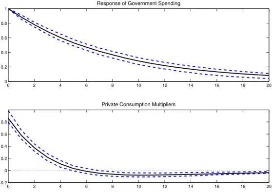
Figure 6 plots the mean and 68 percent probability band for responses of gov-ernment spending and private consumption to a serially correlated shock to Gt
nor-malized to equal $1 in the initial period. We compute impact multipliers to be comparable to empirical work. Private consumption responds strongly on impact, with a mean jump of over 80 cents. The multiplier remains positive for about six quarters before turning mildly negative. Multipliers in this range are reported by Monacelli and Perotti (2008) for U.S. data, though their estimates imply a weak ini-tial response of consumption that gradually builds to a peak 8 to 10 quarters after the shock. Our simple model has little internal propagation, so the large impact effect
13In simulations where the regime realizations produce active monetary and active fiscal policy,
debt temporarily assumes a nonstationary path because neither the monetary or fiscal authority is acting in a manner that ensures long-run solvency. When the doubly active regime persists too long, the solution moves far off the grid for the discretized state space and approximation errors can produce imply economically infeasible solutions. We discard any draws that exhibit such behavior, leaving us with 571 samples of time series.
and rapid decay are to be expected. Nonetheless, the figure shows that the setup in which monetary and fiscal regimes fluctuate over time is capable of generating consumption responses of the magnitude observed in U.S. time series.
8. Simulating Fiscal Simulus: The 2009 ARRA
The American Recovery and Reinvestment Act of 2009 is the fiscal stimulus pack-aged passed by Congress with the primary intention of stabilizing economic activity following the sharp decline in output late in 2008. The total size of the package is $787 billion and comprises both additional government spending and tax cuts. This section illustrates that the likely impact of the stimulus rests with how monetary and fiscal policies are expected to respond going forward.
In line with the focus of the paper thus far, we analyze the impact of the additional purchases contained in the stimulus package. The stimulus package contains spending on infrastructure, healthcare, energy, and so forth and it includes $144 billion in federal transfers to state and local governments. These transfers do not necessarily need to go toward increasing purchases, but instead could be used to avoid tax hikes or borrowing. Following Romer and Bernstein (2009) and Cogan, Cwik, Taylor, and Wieland (2009), we assume that 60 percent of the transfers to state and local governments go toward increasing purchases. Using this assumption, Cogan, Cwik, Taylor, and Wieland (2009) report the increase in government purchases, on a yearly basis, due to the stimulus package.
Figure 7 compares the paths of several variables in response to the path of the additional government purchases from the ARRA as estimated from Cogan, Cwik, Taylor, and Wieland (2009). The government spending stimulus, depicted in the third panel in the left column, is injected into the economy as a sequence of shocks. We compute responses under both AM/PF and PM/AF. Under AM/PF (solid lines), the active monetary response drives up the real rate in response to the increase in purchases. Total output and inflation, however, follow a hump-shape and peak roughly at the same time as the peak in government purchases. Fiscal financing of the increase in spending occurs very gradually, with both debt and taxes above their steady state levels for many years.
Under PM/AF (dashed lines), passive monetary policy allows the real interest rate to fall, so stimulates consumption demand. Inflation peaks nearly 300 basis points
above its steady state level about five quarters after the initial impulse. Relatively high inflation erodes the real value of outstanding debt, leaving it considerably below its level in the AM/PF regime.
To obtain a sense of how much future variability can be attributed to shifts in policy regime, figure 8 reports the mean response of a monte carlo exercise that uses the Cogan, Cwik, Taylor, and Wieland (2009) path for government purchases, but randomly draws over regimes. Dashed lines represent two-standard deviation bands computed at each point in time. The initial regime is set to PM/AF, so the initial rise in government purchases is often occurring under this same regime, since it is relatively persistent. Persistence of the regime causes the mean response of the real rate to fall, but then assumes a less certain path as the effect of some draws of active monetary policy are realized.
8.1. Fiscal Foresight. Table 5 formally quantifies the ARRA path of Cogan, Cwik, Taylor, and Wieland (2009) in terms of output multipliers. One issue that arises in such computations is whether agents fully internalize the future path of govern-ment purchases, or are surprised each period—that is, they have no foresight about the stimulus package. One method to incorporate foresight is to modify the pro-cess for government purchases by adding moving average terms to the government purchase process and convert it to an ARMA(1,5). We calibrate the moving av-erage coefficients using a minimum distance estimator based on the Cogan, Cwik, Taylor, and Wieland (2009) path and impulse response of the ARMA(1,5). Under the ARMA(1,5) process, a shock to purchases implies a path similar to that of the ARRA, except agents have full knowledge of its trajectory. The ARMA(1,5) adds five state variables, which renders the nonlinear solution method for the regime-switching model impractical. To obtain a sense of how important fiscal foresight is, we move to a linear fixed-regime setting.
The top portion of table 5 reports the multipliers under the assumption of no foresight. A similar pattern emerges as in the regime-switching setting following the AR(1) shock, except the multipliers under the PM/AF regime are considerably larger. Under foresight, however, agents have knowledge of the rising level of purchases so substantially revise up their expectations of future inflation in response to a shock. The passive monetary response causes a sharp drop in the real rate and the large present-value multiplier, which is 4.83 after five quarters under PM/AF. In contrast, the monetary authority responds aggressively to the higher inflation in the AM/PF,
which pushes the real rate higher relative to the case of no foresight and dampens the multiplier.
8.2. What If Monetary Policy Becomes Active? In both of the regimes in fig-ure 7, inflation rises. In the regime that probably best describes policy behavior through 2008 and 2009, passive monetary/active fiscal policy, inflation rises substan-tially for several years. A plausible response of the Federal Reserve to rising inflation is to switch to being active. In the absence of a coordinated switch in fiscal policy to a passive stance, both policies would be active, at least for a time. If regime were fixed and both policies were active, no equilibrium would exist. In the present envi-ronment, because agents anticipate the active/active regime will not persist forever, the economy can visit such a regime periodically and temporarily. As the estimated policy rules suggest, the U.S. economy resided in an active/active regime for much of the 1980s [see figure 3].14
Figure 9 superimposes the paths of macroeconomic variables given the government spending associated with the ARRA when policy is doubly active onto the paths in figure 7. Active monetary/active fiscal policies produce markedly different paths for macro variables: inflation rises and remains well above its initial level; output and consumption boom; government debt grows with no tendency to be stabilized. Ac-tive monetary policy attempts to combat the rise in inflation by raising the nominal interest rate sharply, which raises the real interest rate. Although monetary policy continues to exert influence over the real rate, it can no longer use that mechanism to reduce aggregate demand and inflation: rapidly rising debt with no prospect of higher future taxes generates increases in aggregate demand that swamp any poten-tial reduction in demand induced by higher real rates. Ironically, higher real interest rates exacerbate the central bank’s difficulties in controlling inflation by raising debt service, the growth rate of debt, and the resulting positive wealth effects.15
In sum, the failure of fiscal policy to raise taxes and stabilize debt impedes mone-tary policy’s efforts in fighting inflation. Although the economy experiences a boom,
14Davig (2005) studies the implications for empirical tests of the government’s intertemporal
bud-get constraint of an environment in which periodically government debt grows at an unsustainable rate.
15A permanent regime of active monetary and active fiscal policy is unsustainable. This can be
seen in figure 9: the combination of rising debt, falling surpluses, and higher real interest rates are incompatible with the intertemporal equilibrium condition, (30).
it does so by generating chronically higher inflation and a growing ratio of govern-ment debt to GDP. The active/active scenario exemplifies the need for monetary and fiscal policy to work together to control inflation.
9. Conclusion
This paper has embedded estimated Markov-switching rules for U.S. monetary and fiscal policy into an otherwise conventional calibrated DSGE model with nom-inal rigidities to deliver some quantitative predictions of the impacts of government spending increases. When monetary and fiscal policy regimes vary—from active monetary/passive fiscal to passive monetary/active fiscal to doubly passive to dou-bly active—government spending multipliers can vary widely. An increase in govern-ment spending of $1 in present value raises output by $0.80 in present value under AM/PF, while it raises output by as much as $1.80 in present value when monetary policy is passive. In our simple model, this translates into adecrease in consumption of $0.20 in present value under AM/PF, but and increase in consumption of about $0.80 in present value under passive monetary policy.
The paper also simulates the general equilibrium impacts of the government spend-ing path implied by the 2009 American Recovery and Reinvestment Act. When the government spending path is modeled as a sequence of shocks to spending, the present-value multiplier for output is about $0.68 under a fixed regime of AM/PF, while it can be well over $3.00 in a fixed PM/AF regime. If the government spending path is treated as foreseen by economic agents—because the path is announced by the passage of the Act—the present-value multiplier for output falls somewhat when the regime is AM/PF, but it rises to nearly $5.00 in the short run when policy obeys a PM/AF regime.
Appendix A. Data Description: Fiscal Variables
The fiscal policy variables we use in estimating the switching fiscal rule (25) are at a quarterly frequency and defined as follows:
• τt = (Federal Receipts - Federal Transfers)/(Nominal GDP) – Federal Receipts: Line 1 of NIPA Table 3.2
– Federal Transfers: Line 21 of NIPA Table 3.2
– Nominal GDP: Line 1 of NIPA Table 1.1.5 • bt=
3
P j=0
(Market value of privately held gross federal debt)t−j/(Nominal GDP)t−j
– Debt series available from Federal Reserve Bank of Dallas website • yt = ln(Nominal GDP/Nominal CBO potential GDP)
– Nominal CBO potential GDP available from Congressional Budget Office website
• gt = (Nominal Federal government consumption expenditures and gross
in-vestment)/(Nominal GDP)
– Nominal Federal government consumption expenditures and gross in-vestment: Line 21 of NIPA Table 1.1.5
References
Aiyagari, S. R., and M. Gertler (1985): “The Backing of Government Debt and Monetarism,” Journal of Monetary Economics, 16(1), 19–44.
Barro, R. J., and R. G. King (1984): “Time-Separable Preferences and
Intertemporal-Substitution Models of Business Cycles,”Quarterly Journal of Eco-nomics, 99(4), 817–839.
Baxter, M., and R. G. King (1993): “Fiscal Policy in General Equilibrium,”
American Economic Review, 83(3), 315–334.
Bianchi, F.(2009): “Regime Switches, Agents’ Beliefs, and Post-World War II U.S. Macroeconomic Dynamics,” Manuscript, Princeton University.
Bilbiie, F. (2008): “Non-Separable Preferences, Fiscal Policy Puzzles and Inferior Goods,” forthcoming in Journal of Money, Credit and Banking.
Blanchard, O. J., and R. Perotti (2002): “An Empirical Characterization of the Dynamic Effects of Changes in Government Spending and Taxes on Output,”
Quarterly Journal of Economics, 117(4), 1329–1368.
Board of Governors of the Federal Reserve System (2008): “Press
Re-lease: Federal Open Market Committee,” October 29.
Bouakez, H., and N. Rebei(2007): “Why Does Private Consumption Rise After a Government Spending Shock?,”Canadian Journal of Economics, 40(3), 954–979. Branson, W. H.(1989): Macroeconomic Theory and Policy. Harper and Row, New
York, 3rd edn.
Calvo, G. A. (1983): “Staggered Prices in a Utility Maximizing Model,” Journal of Monetary Economics, 12(3), 383–398.
Chari, V. V., P. J. Kehoe, and E. R. McGrattan (2000): “Sticky Price
Models of the Business Cycle: Can the Contract Multiplier Solve the Persistence Problem?,” Econometrica, 68(5), 1151–1179.
Chung, H., T. Davig, and E. M. Leeper (2007): “Monetary and Fiscal Policy Switching,”Journal of Money, Credit and Banking, 39(4), 809–842.
Clarida, R., J. Gali,andM. Gertler(1999): “The Science of Monetary Policy: A New Keynesian Perspective,”Journal of Economic Literature, 37(4), 1661–1707. Cochrane, J. H. (2005): “Money as Stock,” Journal of Monetary Economics,
52(3), 501–528.
Cogan, J. F., T. Cwik, J. B. Taylor, and V. Wieland(2009): “New Keyne-sian versus Old KeyneKeyne-sian Government Spending Multipliers,” Manuscript, Stan-ford University.
Congressional Budget Office (2009): A Preliminary Analysis of the Presi-dent’s Budget and an Update of CBO’s Budget and Economic Outlook, vol. March. CBO, Washington, D.C.
Davig, T. (2005): “Periodically Expanding Discounted Debt: A Threat to Fiscal Policy Sustainability?,”Journal of Applied Econometrics, 20(7), 829–840.
Davig, T., and E. M. Leeper(2006): “Fluctuating Macro Policies and the Fiscal Theory,” inNBER Macroeconomics Annual 2006, ed. by D. Acemoglu, K. Rogoff,
and M. Woodford, pp. 247–298. MIT Press, Cambridge.
(2007): “Generalizing the Taylor Principle,” American Economic Review, 97(3), 607–635.
Dixit, A. K., and J. E. Stiglitz (1977): “Monopolistic Competition and Opti-mum Product Diversity,”American Economic Review, 67(3), 297–308.
Farmer, R. E. A., T. Zha,and D. Waggoner(2009): “Understanding Markov-Switching Rational Expectations Models,” NBER Working Paper No. 14710. Favero, C. A., and T. Monacelli (2005): “Fiscal Policy Rules and Regime
(In)Stability: Evidence from the U.S.,” Manuscript, IGIER.
Gali, J., J. D. Lopez-Salido,andJ. Valles(2007): “Understanding the Effects of Government Spending on Consumption,” Journal of the European Economic Association, 5(1), 227–270.
Greenwood, J., Z. Hercowitz, and G. W. Huffman (1988): “Investment,
Capacity Utilization, and the Real Business Cycle,” American Economic Review, 78(3), 402–417.
Kim, S. (2003): “Structural Shocks and the Fiscal Theory of the Price Level in the Sticky Price Model,” Macroeconomic Dynamics, 7(5), 759–782.
King, R. G., C. I. Plosser, and S. T. Rebelo (1988): “Production, Growth, and Business Cycles: I. The Basic Neoclassical Model,”Journal of Monetary Eco-nomics, 21(March/May), 195–232.
Leeper, E. M. (1991): “Equilibria Under ‘Active’ and ‘Passive’ Monetary and Fiscal Policies,”Journal of Monetary Economics, 27(1), 129–147.
Leeper, E. M., and T. Yun (2006): “The Fiscal Theory of the Price Level: Background and Beyond,”International Tax and Public Finance, 13(4), 373–409. Leeper, E. M., and T. Zha (2003): “Modest Policy Interventions,” Journal of
Monetary Economics, 50(8), 1673–1700.
Linnemann, L.(2006): “The Effect of Government Spending on Private Consump-tion: A Puzzle?,” Journal of Money, Credit and Banking, 38(7), 1715–1735.
Lubik, T. A., and F. Schorfheide (2004): “Testing for Indeterminacy: An Application to U.S. Monetary Policy,” American Economic Review, 94(1), 190– 217.
Lucas, Jr., R. E. (1988): “Money Demand in the United States: A Quantitative Review,”Carneige-Rochester Conference Series on Public Policy, pp. 137–168.
Mankiw, N. G., and L. H. Summers (1986): “Money Demand and the Effects
of Fiscal Policies,” Journal of Money, Credit, and Banking, 18(4), 415–429. Monacelli, T., and R. Perotti (2008): “Fiscal Policy, Wealth Effects, and
Markups,” NBER Working Paper No. 14584.
Mountford, A., and H. Uhlig (2009): “What Are the Effects of Fiscal Policy Shocks?,” forthcoming in Journal of Applied Econometrics.
Perotti, R. (2007): “In Search of the Transmission Mechanism of Fiscal Pol-icy,” in NBER Macroeconomics Annual 2007, ed. by D. Acemoglu, K. Rogoff, and
M. Woodford, vol. 22, pp. 169–226. University of Chicago Press, Chicago, NBER Working Paper No. 13143.
Ramey, V. A. (2007): “Identifying Government Spending Shocks: It’s All in the Timing,” Manuscript, University of California, San Diego.
Ramey, V. A., and M. D. Shapiro (1998): “Costly Capital Reallocation and the Effects of Government Spending,” Carneige-Rochester Conference Series on Public Policy, 48, 145–194.
Ravn, M. O., S. Schmitt-Grohe, andM. Uribe(2007): “Explaining the Effects of Government Spending Shocks on Consumption and the Real Exchange Rate,” NBER Working Paper No. 13328.
Romer, C., and J. Bernstein (2009): The Job Impact of the American Recovery and Reinvestment Plan. Obama Transition Team, Washington, D.C., January 9. Rotemberg, J. J., and M. Woodford(1997): “An Optimization-Based
Econo-metric Framework for the Evaluation of Monetary Policy,” in NBER Macroeco-nomics Annual 1997, ed. by B. S. Bernanke, and J. J. Rotemberg, pp. 297–346.
MIT Press, Cambridge, MA.
Sargent, T. J., and N. Wallace (1981): “Some Unpleasant Monetarist Arith-metic,” Federal Reserve Bank of Minneapolis Quarterly Review, 5(Fall), 1–17. Sims, C. A. (1988): “Identifying Policy Effects,” in Empirical Macroeconomics for
Interdependent Economics, ed. by R. C. Bryant, pp. 308–321. The Brookings In-stitution, Washington, DC.
Svensson, L. E. O., and N. Williams (2007): “Monetary Policy with Model Uncertainty: Distribution Foreacast Targeting,” Manuscript, University of Wis-consin.
(2008): “Optimal Monetary Policy Under Uncertainty: A Markov Jump-Linear-Quadratic Approach,” Federal Reserve Bank of St. Louis Review, 90(4), 275–293.
Wallace, N.(1981): “A Modigliani-Miller Theorem for Open-Market Operations,”
American Economic Review, 71(3), 267–274.
Woodford, M. (1998): “Control of the Public Debt: A Requirement for Price Stability?,” in The Debt Burden and Its Consequences for Monetary Policy, ed. by G. Calvo, and M. King, pp. 117–154. St. Martin’s Press, New York.
(2003): Interest and Prices: Foundations of a Theory of Monetary Policy. Princeton University Press, Princeton, N.J.
Active Passive State SM t = 1 StM = 2 StM = 3 StM = 4 α0 .0068 .0068 .0058 .0058 (.0005) (.0005) (.0002) (.0002) απ 1.2936 1.2936 .5305 .5305 (.062) (.062) (.02) (.02) αy .0249 .0249 .0485 .0485 (.005) (.005) (.0046) (.0046) σ2
r 1.61615e-005 9.18552e-007 2.07447e-005 5.51202e-007
(9.67157e-006) (1.95885e-006) (3.4185e-006) (1.75348e-006) Table 1. Monetary policy rule estimates. Log likelihood value = −1079.52.
State SF t = 1 StF = 2 γ0 .029 .004 (.0025) (.0036) γb .071 -.025 (.0044) (.0066) γy .498 .324 (.025) (.035) γg .409 1.022 (.026) (.030) σ2 τ 4.25e-5 4.98e-005 (6.82e-6) (8.58e-6)
P V(∆Y)
P V(∆G) after
Regime 5 quarters 10 quarters 25 quarters ∞
AM/PF .79 .80 .84 .86 PM/PF 1.64 1.51 1.39 1.37 PM/AF 1.72 1.58 1.4 1.36 Note: P V(∆C) P V(∆G) = P V(∆Y) P V(∆G) −1.
Table 3. Present value multipliers from the regime-switching model. %∆P after
Regime 5 quarters 10 quarters 25 quarters
AM/PF .76 1.34 2.37
PM/PF 2.19 3.18 3.98
PM/AF 2.41 3.40 3.95
Table 4. Impact of a 3% increase in government purchases on the price level in the regime-switching model.
P V(∆Y)
P V(∆G) after
Regime 5 quarters 10 quarters 25 quarters ∞
No Foresight—AR(1) AM/PF .68 .68 .68 .68 PM/AF 3.29 2.88 2.41 2.3 Foresight—ARMA(1,5) AM/PF .52 .61 .63 .63 PM/AF 4.83 3.10 2.31 2.17
Table 5. Present value multipliers from the fixed-regime model; with and without foresight.
1950 1960 1970 1980 1990 2000 2010 0
0.5 1
Active Monetary Policy, High σ
Filtered Probabilities Smoothed Probabilities 1950 1960 1970 1980 1990 2000 2010 0 0.5 1
Active Monetary Policy, Low σ
1950 1960 1970 1980 1990 2000 2010
0 0.5 1
Passive Monetary Policy, High σ
1950 1960 1970 1980 1990 2000 2010
0 0.5 1
Passive Monetary Policy, Low σ
1950 1960 1970 1980 1990 2000 2010 0 0.1 0.2 0.3 0.4 0.5 0.6 0.7 0.8 0.9 1
Probability of Active Fiscal Policy
Filtered Probabilities Smoothed Probabilities
Figure 2. U.S. Fiscal Regime Probabilities
1950 1955 1960 1965 1970 1975 1980 1985 1990 1995 2000 2005
AM,PF − Ricardian AM,AF − Explosive PM,PF − Indeterminacy PM,AF − Fiscal Theory
0 5 10 15 20 25 30 −0.5 0 0.5 1 1.5 Output Gap % 0 5 10 15 20 25 30 −0.2 0 0.2 0.4 0.6 Consumption % 0 5 10 15 20 25 30 0 100 200 300 Inflation basis points 0 5 10 15 20 25 30 −50 0 50 Real Rate basis points 0 5 10 15 20 25 30 0 100 200 Nominal R basis points 0 5 10 15 20 25 30 −1 0 1 2 Debt (level) % 0 5 10 15 20 25 30 0 2 4 Gov Purchases % 0 5 10 15 20 25 30 −1 0 1 2 3 % Taxes AM/PF PM/PF PM/AF
Figure 4. Responses to a shock to government purchases, condition-ing on remaincondition-ing in the prevailcondition-ing regime. In deviations from steady state. Time units in quarters.
0 5 10 15 20 25 30 −0.5 0 0.5 1 1.5 2 Debt (level) % 0 5 10 15 20 25 30 −40 −30 −20 −10 0 10 Primary Surplus % 0 5 10 15 20 25 30 −1.5 −1 −0.5 0 0.5 1 1.5 PV Primary Surplus
%, weighted by share of debt
0 5 10 15 20 25 30 −0.5 0 0.5 1 1.5 2 2.5 3
%, weighted by share of debt
PV Seigniorage
AM/PF PM/PF PM/AF
Figure 5. Responses of fiscal variables to a shock to government pur-chases, conditioning on remaining in the prevailing regime. In devia-tions from steady state. Time units in quarters.
0 2 4 6 8 10 12 14 16 18 20 0 0.2 0.4 0.6 0.8 1
Response of Government Spending
0 2 4 6 8 10 12 14 16 18 20 −0.2 0 0.2 0.4 0.6 0.8
Private Consumption Multipliers
Figure 6. Government spending impact multipliers for consumption from VAR fit to simulated data from the regime-switching model. Time units in quarters.
0 5 10 15 20 25 30 35 −0.5 0 0.5 1 1.5 Output Gap % 0 5 10 15 20 25 30 35 −0.2 0 0.2 0.4 0.6 Consumption % 0 5 10 15 20 25 30 35 0 100 200 300 Inflation basis points 0 5 10 15 20 25 30 35 −50 0 50 Real Rate basis points 0 5 10 15 20 25 30 35 0 2 4 Gov Purchases % 0 5 10 15 20 25 30 35 −1 0 1 2 3 Taxes % 0 5 10 15 20 25 30 35 0 2 4 Debt % 0 5 10 15 20 25 30 35 −40 −20 0 20 % Primary Surplus AM/PF PM/AF
Figure 7. Impacts of the government spending path implied by the American Recovery and Reinvestment Act of 2009, conditioning on either active monetary/passive fiscal (AM/PF) policy (solid lines) and passive monetary/active fiscal (PM/AF) policy (dashed lines) regime. In deviations from steady state. Time units in quarters.
0 5 10 15 20 25 −0.5 0 0.5 1 1.5 Output Gap % 0 5 10 15 20 25 −0.5 0 0.5 1 Consumption % 0 5 10 15 20 25 −100 0 100 200 300 Inflation basis points 0 5 10 15 20 25 −100 −50 0 50 Real Rate basis points 0 5 10 15 20 25 0 2 4 Gov Purchases % 0 5 10 15 20 25 −2 0 2 Taxes % 0 5 10 15 20 25 −1 0 1 2 Debt (Level) % 0 5 10 15 20 25 −60 −40 −20 0 Primary Surplus %
Figure 8. Simulating the 2009 ARRA randomly drawing over future monetary and fiscal regimes, including two-standard deviation error bands. Initial regime is passive monetary/active fiscal. In deviations from steady state. Time units in quarters.
0 5 10 15 20 25 30 35 −0.5 0 0.5 1 1.5 Output Gap % 0 5 10 15 20 25 30 35 −0.4 0 0.4 0.8 Consumption % 0 5 10 15 20 25 30 35 0 100 200 300 Inflation basis points 0 5 10 15 20 25 30 35 −50 0 50 Real Rate basis points 0 5 10 15 20 25 30 35 0 2 4 Gov Purchases % 0 5 10 15 20 25 30 35 −1 0 1 2 3 Taxes % 0 5 10 15 20 25 30 35 0 5 10 Debt % 0 5 10 15 20 25 30 35 −60 −40 −20 0 20 Primary Surplus % PM/AF AM/AF AM/PF
Figure 9. Impacts of the government spending path implied by the American Recovery and Reinvestment Act of 2009, conditioning on active monetary/active fiscal (AM/AF) regime (dotted-dashed lines). Also depicted are active monetary/passive fiscal (AM/PF) policy (solid lines) and passive monetary/active fiscal (PM/AF) policy regimes (dashed lines). In deviations from steady state. Time units in quarters.