The Predictive Value of Inequality Measures for Stock Returns: An
Analysis of Long-Span UK Data Using Quantile Random Forests
Submission: February 2018 Resubmission: August 2018
Abstract
We contribute to research on the predictability of stock returns in two ways. First, we use quantile random forests to study the predictive value of various consumption-based and income-based inequality measures across the quantiles of the conditional distribution of stock returns. Second, we examine whether the inequality measures, measured at a quarterly frequency, have out-of-sample predictive value for stock returns at three different forecast horizons. Our results suggest that the inequality measures have predictive value for stock returns in sample, but do not systematically predict stock returns out of sample.
JEL classification: C53; G17
1
Introduction
The existing literature on predicting stock returns in developed and developing countries, based on a wide array of models and predictors, is vast, to say the least (see for example, Rapach et al., 2005, 2013, Sousa et al., 2016, Aye et al., 2017, Jordan et al., 2017, among others). On one hand, practitioners in finance require real-time forecasts of stock returns for asset-allocation decisions. On the other hand, academics in finance are interested in stock-return predictability because predictability has important implications for tests of market efficiency and, thereby, may help to produce more realistic asset-pricing models (Rapach and Zhou, 2013). Predicting stock returns, however, is highly challenging because stock returns inherently contain a sizable unpredictable component and, hence, forecasting performance varies across the countries and sample periods studied and models and predictors used. This paper contributes to research on stock-return predictability by using a novel technique, quantile random forests, to examine the relationship between inequality and stock returns.
With an upward trend in both income and wealth inequality globally (Piketty and Saez, 2014), the question of whether inequality plays a role in stock-market developments becomes increas-ingly pertinent. Intuition suggests that higher inequality is likely to lead to lower stock-market investments (due to lower participation), thus affecting stock prices. Solid economic reasoning that inequality can predict asset prices has been recently provided by many studies. For exam-ple, Gollier (2001) shows that in a model with complete markets but with agents having concave risk tolerance (i.e., dropping the assumption of constant relative risk-aversion (CRRA))1 wealth inequality increases the equity premium, i.e., stock returns relative to the return on a risk-free asset. Alternatively, Constantinides and Duffie (1996) maintain the CRRA assumption but in-troduce incomplete markets. In their model, investors are identical ex ante but face uninsurable idiosyncratic income shocks which, in turn, lead to ex post dispersion of investor incomes. As a result, investors demand a higher risk premium for assets that provide a poor hedge against
1Cochrane (2005) points out that when agents have identical CRRA preferences and markets are complete
idiosyncratic income shocks. If inequality is correlated with the magnitude of the uninsurable idiosyncratic income risk and equities are a poor hedge against inequality (as shown by Ait-Sahalia et al., 2004) then higher inequality causes a higher equity-risk premium. In addition, political channels can lead to inequality causing the equity premium in an indirect fashion. On the one hand, Persson and Tabellini (1994) indicate that as inequality grows politicians targeting the median voter have incentives to tax investment for the purpose of wealth redistribution, which causes higher risk premia (Croce et al., 2012; Gomes et al., 2012). On the other hand, Alesina and Perotti (1996) argue that income inequality leads to political uncertainty, which increases the equity premium as described in the works of Pástor and Veronesi (2012, 2013).
Given that there are many possible theoretical channels through which inequality can affect stock markets, it is important to discuss work that examines some of these theoretical predictions. First, Brogaard et al., (2015) find that, after controlling for the dividend-price ratio, higher income in-equality (measured by the Gini coefficient) predicts not only a significantly higher equity-risk premium but also risk premia on long-term government and corporate bonds.2 Moreover, Bro-gaard et al. (2015) show that the inclusion of the Gini coefficient in a one-year stock-return predictability regression that includes the dividend-price ratio more than doubles the explanatory power (with the adjusted-R2 increasing from 5.6% to 14.8%). These findings are also shown to be robust to alternative measures of inequality and other common financial and real-business cycle predictors of returns generally used in this literature. Second, Christou et al., (2017) in-vestigate whether the post-tax-and-transfer growth rate of the Gini index helps to predict the equity premium in the G7 countries (Canada, France, Germany, Italy, Japan, United Kingdom, and United States) using a panel-data-based predictive framework, which controls for hetero-geneity, cross-sectional dependence, persistence, and endogeneity. Christou et al., (2017) show that, while in general time-series based predictive regression models fail to beat the historical average, panel-data models beat this benchmark in a statistically significant fashion for all the seven countries. This result highlights the importance of pooling information when trying to
2The authors find that a one-standard deviation increase in Gini coefficient is associated with an increase of
forecast stock returns based on a measure of inequality.3 Both papers, not surprisingly, analyzed predictability of stock returns at the annual frequency using inequality data that is generally also available at the same frequency.
Against this backdrop, the objective of this paper is to investigate for the first time whether inequality forecasts United Kingdom (UK) stock returns. We examine data at the quarterly fre-quency, the highest possible, over 1977Q1 to 2016Q1 using both out of sample and in sample approaches as well as considering income-based and consumption-based inequality measures. Further, we introduce quantile random forests (Meinshausen, 2006) into the literature on stock-return predictability. Quantile random forests have the advantage of being a flexible data-driven modeling framework. Given that inequality may affect stock returns through a variety of chan-nels and in a variety of ways, quantile random forests are capable of capturing such complex nonlinear effects in a natural way. In addition, quantile random forests render it possible to cap-ture any interaction effects of inequality with a wide-array of predictors (as in Jordan et al., 2017) generally used in the literature on stock-returns predictability. Finally, as with a more standard quantile regression model (Koenker, 2005), quantile random forests allow the predictive value of inequality for stock returns to be traced out along the quantiles of the conditional distribution of stock returns. This is advantageous for investors who are interested in studying the implications of a potential stock-returns-inequality nexus for the management of tail events.
We briefly describe quantile random forests in Section2. We describe our data in Section3. We describe our empirical analysis in Section4. We conclude in Section5.
2
Quantile Random Forests
A regression tree consists of a root, interior nodes, and terminal nodes (the leaves; for an intro-duction to regression trees, see Hastie et al., 2009; for recent applications of regression trees in
3In a somewhat related paper, Johnson (2012) analyzes the cross-sectional pricing implications associated with
the risk of inequality. The analysis shows that stock returns that comove more with inequality attract a negative premium. In other words, investors are willing to pay a higher price for assets which tend to provide a better hedge against the risk of falling income status.
economics, see Döpke et al. 2017 and Behrens et al. 2018). The nodes recursively partition the space of predictors,xt,t =1, ...,N, into rectangular subspaces in a top-down and binary way. A
leaf of a regression tree represents a rectangular subspace of relative homogeneity of stock re-turns,rt+h, wherehdenotes the forecast horizon. The formation of rectangular subspaces starts at the top level of a regression tree by choosing the partitioning predictor,s, and the partitioning point,z, to form the two regionsR1(s,z) ={xt,s|xt,s≤z}andR2(s,z) ={xt,s|xt,s>z}by solving
mins,z{RSS1+RSS2}, whereRSSk=∑xt,s∈Rk(s,z)(rt+h,i−r¯t+h,k)
2, with ¯r
t+h,k=mean{rt+h,i|xt,s∈ Rk(s,z)},k=1,2,xt,s∈Rk denotes that the period-t realization of predictorsbelongs to region
Rk, andrt+h,iare the stock returns in regionk. This search-and-split process then proceeds in a
recursive and hierarchical way until every leaf contains a minimum number of observations or some maximal tree size is reached, both are defined in advance.
A random regression tree is a regression tree that is grown by choosing only a random subset of the predictors in every step of the search-and-split process. A random forest is an ensemble of random regression trees, where every single random regression tree that is member of this ensemble is estimated on a boostrapped sample of the data (Breiman, 2001). Choosing a ran-dom subset of the predictors and forming a ranran-dom forest that consists of bootstrapped ranran-dom regression trees has the advantages that it curbs the influence of individual influential predictors on the predictions and decorrelates the predictions form individual random regression trees. Meinshagen (2006) extends the concept of random forests to quantile random forests. He ob-serves that the search-and-split process implies that at the leaves every observation of stock returns receives a weightwt=1{xt,s∈Rk(s,z)}/(#{j:xj,s∈Rk(s,z)}), where1is the indicator
func-tion. The prediction of stock returns is then ˆrt+h=∑Nt=1wtrt+h. When estimating a random
for-est, in turn, the weight attached to observationt of stock returns is defined aswtB=B−1∑Bi=1wt,
and the prediction of stock returns is given by ˆrt+h=∑t=1N wtBrt+h, where B denotes the
num-ber of bootstrapped random regression trees. Equipped with these weights, a quantile random forest stores not only information on the mean of stock returns at the leaves (as a conventional regression tree does) but rather keeps all observations of stock returns, and then uses this infor-mation to compute an estimate, ˆP(rt+h ≤r|xt) =F(r|xˆ t), of the conditional distribution
func-tion of stock returns. This estimate is computed as ˆF(r|xt) =∑Nt=1wBt1rt+h≤r. The α-quantile of the conditional distribution function is defined such that the probability that stock returns is smaller thanQα, givenxt, is equal to α, with an estimate of theα-quantile being computed as
ˆ
Qα(xt) =inf{r: ˆF(r|xt)≥α}.
3
Data
Quarterly data is collected and computations are made from March (Q1) 1977 until March (Q1) 2016. The inequality data is for income equivalized by dividing by the square root of the number of people in a household and total consumption per capita of a household. The three measures of inequality used are the Gini coefficient, standard deviation (of the data in natural logarithms), and the difference between the 90th and 10th percentile (with the data in natural logarithms). The inequality measures are calculated using survey data on income and consumption from the family expenditure survey.4 Further details on the construction of the data and the survey are documented in Mumtaz and Theophilopoulou (2017).5 We abbreviate the three income-based inequality measures as YI1, YI2, and YI3. The three consumption-based inequality measures are denoted as CI1, CI2, and CI3.
The UK stock-return data and (auxiliary) predictors are primarily collected from Thomson Datas-tream. The log change in the UK Market Return Index is used to estimate stock return.6The other predictors used are key candidate variables drawn from valuation fundamentals and macroeco-nomics, which follow Goyal and Welch (2008) and Jordan et al. (2017). Specifically we include the dividend-price ratio, dividend yield, earnings-price ratio, book-market ratio, T-Bill rate, in-flation, and stock variance. Details on the construction of the (auxiliary) predictors can be found at the end of the paper (Data Appendix).
4The data is downloadable from:https://discover.ukdataservice.ac.uk/series/?sn=200016 and
https://discover.ukdataservice.ac.uk/series/?sn=2000028.
5We would like to thank Professor Haroon Mumtaz for kindly sharing the inequality data with us.
4
Empirical Analysis
We use the R programming environment for statistical computing for our empirical analysis (R Development Core Team 2017) and the add-on-package “quantregForest ” (Meinshausen, 2016) for estimation of quantile random forests. We use quantile random forests to compute both in-sample and out-of-sample forecasts of stock returns one-quarter ahead, two-quarters ahead, and one-year ahead (h =1,2,4). For computing out-of-sample forecasts, we use a recursive estimation window. The first estimation window uses data up to and including 1996Q4, then we add data for 1997Q1 to the estimation window, and so on until we reach the end of the sample period. We present results for quantile random forests that consist of 750 random regression trees. We set the minimum number of observations per terminal node to ten, and we use one-third of the predictors for random splitting. Using 500 or 1000 trees or fixing the maximum number of terminal nodes to ten (rather than the number of observations per terminal node) leads to qualitatively similar results (not reported, but available upon request).
Following Gupta et al. (2017), we compare the predictive value of forecasts by extending the approach proposed by Fair and Shiller (1990) to a quantile-regression setting (on quantile regres-sions, see Koenker and Bassett, 1978; Koenker, 2005). To this end, we estimate for every quan-tile parameter α and h, the following quantile regression model γα∗,h=arg min
γα,h
∑tL(α,rt+h− Xt+1γα,h), where the summation runs over the available in-sample or out-of-sample predictions,
Xt+1γα,h=γ0,α,h+γ1,α,hrˆt+h+γ2,α,hrˆt+hwo , andL is the usual quantile regression loss function
(that is, the “check function”), and ˆrt+hwo denotes a benchmark forecast implied by a model that does not feature any inequality measure in the vector of predictors. If the forecasts, ˆrt+h, of the model featuring an inequality measure in the vector of predictors have predictive value forrt+h, and the predictive value of the benchmark forecasts, ˆrt+hwo , is fully contained in ˆrt+h, thenγ1,α,h
should be significantly different from zero whileγ2,α,hshould be insignificant. If both forecasts
contain non-overlapping information thenγ1,α,handγ2,α,hshould be significantly different from
zero. If both forecasts do not have predictive value then bothγ1,α,handγ2,α,hshould not be
andγ2,α,hare not separately identified (see Fair and Shiller, 1990, page 377).
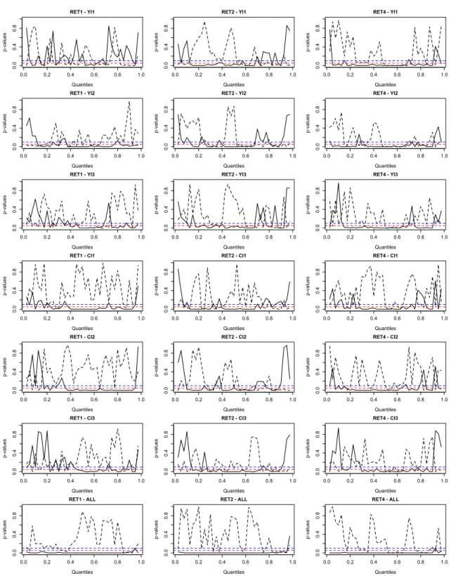
Figure 1plots bootstrapped (1,000 simulation runs) p-values of in-sample tests of the null hy-potheses thatγ1,α,h(solid line) andγ2,α,h(dashed line) are not significantly different from zero.
We present results for forecasts from seven different models at three different forecast horizons (we look at stock returns 1, 2, and 4 quarters ahead). For example, the solid line in the panel entitled RET1-YI1 represents, for stock returns one quarter ahead, the results for the forecasts implied by a model that features, in addition to the other auxiliary predictors, the inequality mea-sure YI1 in the vector of predictors. The dashed line represents the results for the benchmark forecasts implied by a model that does not feature any of our inequality measures in the vector of predictors. Because we analyze six different inequality measures, we present results for six dif-ferent models. In addition, we present results for a seventh model that features all six inequality measures in the vector of predictors.
−Please include Figure1about here.−
The general message conveyed by the in-sample results is that the inequality measures improve the predictive value of the models. The model that features all inequality measures in the vector of predictors produces p-values below the conventional thresholds of 5% and 10% at most quan-tiles and at all three forecast horizons. The p-values for the models that feature only one of the inequality measures as a predictor are more volatile across quantiles than those for the model that features all inequality measures as predictors. Still, the models tend to produce more significant results than the model that excludes the inequality measures from the vector of predictors.
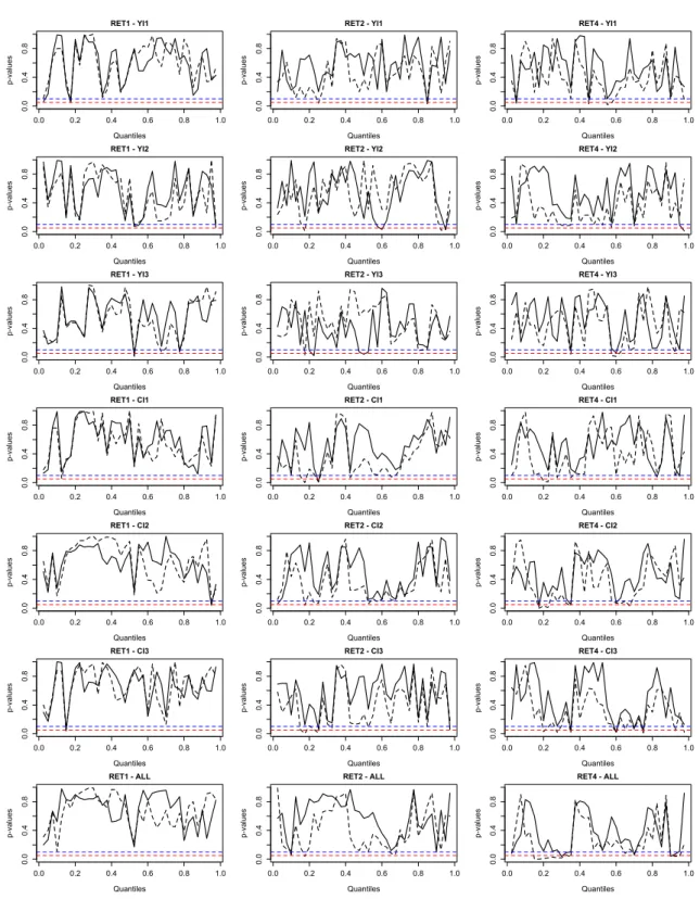
−Please include Figure2about here.−
Figure2plots bootstrapped p-values of out-sample tests. The results are in stark contrast to the results of the in-sample tests. The p-values are rather volatile across quantiles and scratch the 5% and 10% thresholds only occasionally. The instability across quantiles and (to a great extent) insignificance of the results holds at all three forecast horizons and irrespective of whether we
include only a single or all six inequality measures in the vector of predictors. Taken together, our results corroborate the results of Christou et al. (2017) insofar as they find, for annual data, no evidence of out-of-sample predictability when they undertake a time-series analysis.
We obtain similar results (not reported, but available from the authors upon request) when we analyze a somewhat shorter (beginning in 2000Q1) and a longer (starting in 1990Q1) out-of-sample forecasting period. Moreover, the results do not change qualitatively when we replace the recursive-estimation window with a rolling-estimation window. Experiments with a model that features realized volatility of stock returns as a predictand rather than as a predictor show that also for such a model there is no strong and robust evidence of out-of-sample predictability.7 Another point one might wonder about is whether there is an impact on stock returns from the first difference of the inequality measures because a shock to inequality could create an unanticipated return, while the level of inequality primarily impacts the expected return. When we use the first difference of the inequality measures to estimate quantile random forests there is no systematic evidence that the inequality measures strengthen out-of-sample predictability of stock returns. Yet another concern is whether excluding forecasts for the period of the financial and economic crisis of 2007/2008 changes our results. In order to inspect the impact of the financial and economic crisis more closely, we estimate two versions of the Fair-Shiller quantile regression models. In the first version, we only use out-of-sample forecasts up to and including 2006Q4. In the second version, we exclude out-of-sample forecasts for the period from 2007Q1 to 2009Q4. Again, there is no systematic evidence of out-of-sample predictability of stock returns. As for the in-sample results, we reestimate the quantile-random-forest model but exclude data for the
7Another aspect that is relevant for the evaluation of out-of-sample forecasts (especially regarding their
useful-ness in practice) is that the inequality measures should be released at or prior to when a forecast is made. While the surveys used by Mumtaz and Theophilopoulou (2017) are at an annual frequency, the authors assign households to different quarters within a year based on the date of survey interviews. Knowing the timing of the survey interviews, they can calculate the measures of inequality at a quarterly frequency. As a robustness check, however, we accounted for the fact that data on inequality for a specific year and, hence, for the quarters of that particular year will only be available at the beginning of the next year. When we account for a publication lag of four quarters, the results (not reported, but available from the authors upon request) of the out-of-sample tests do not change qualitatively.
period from 2007Q1 to 2009Q4. Results are qualitatively similar to those reported in Figure1. The in-sample results, thus, are not strong only because they include the crisis period (that is, due to a potential look-ahead bias).
It is important to check whether the lack of out-of-sample predictability is an artefact of the forecasts computed by means of quantile random forests. In order to consider this possibility, we compute forecasts by means of (i) a quantile boosting model as described in Pierdzioch et al. (2016), and, (ii) a standard “kitchen-sink” quantile regression model that always contains all regressors (that is, the auxiliary predictors plus the inequality measure being studied). We then estimate the Fair-Shiller quantile regression models for the forecasts implied by such a model. Again, we do not find systematic evidence of out-of-sample predictability.
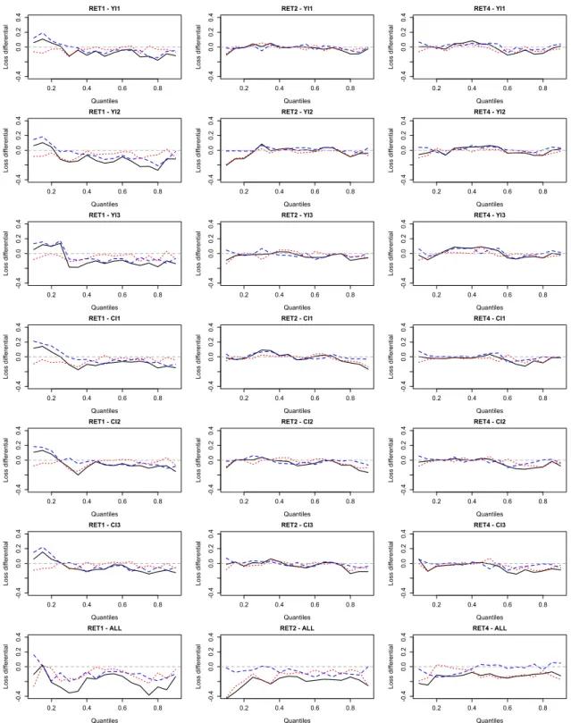
−Please include Figure3about here.−
Finally, we compare quantile random forests with the quantile boosting model and the standard quantile regression model in terms of their out-of-sample forecast performance. To this end, we use the “check function” as our loss function. Specifically, we compute, for every single one of the three forecasting models and for the various quantile parameters, the cumulated loss defined as the sum of the values taken by the loss function over the out-of-sample period. We then as-sess relative forecasting performance by computing the difference between the cumulated losses. Figure3 shows that, except for small quantile parameters, quantile random forests tend to per-form better than the competitor models forh=1, and that the quantile boosting model performs better than both quantile random forests and the quantile regression model. Forh=2 andh=4, and when we consider only one inequality measure at a time, the two competitor models show a slightly better performance for various quantile parameters in the range between approximately 0.2 and 0.5. The competitor models, however, tend to lose in terms of relative performance for larger quantile parameters. When we simultaneously consider all inequality measures, quantile random forests show the strongest relative forecasting performance. Only the quantile boosting model performs better than quantile random forests for some quantile parameters in the range between roughly 0.4 and 0.8, and only forh=4.
5
Concluding Remarks
Inequality of income and wealth has been on the rise in many countries around the world. This can potentially have serious social and economic consequences but the impact on financial mar-kets has been largely unexplored. Notable exceptions include Gollier (2001) and Ait-Sahalia et al. (2004), who identify mechanisms through which higher inequality leads to a higher equity premium and thus lower stock prices. Brogaard et al. (2015) and Christou et al. (2017) examine whether inequality predicts stock returns in the US and the G7 respectively. Using annual data they find a statistically significant relationship.
This paper extends the literature by providing rigorous evidence on the relationship between inequality and the conditional distribution of stock returns in the UK. We implement a novel technique, quantile random forests, which enables predictability across the whole spectrum of the conditional distribution of stock returns to be examined. Quantile random forests is a flexible data-driven nonparametric method which can accomodate interactions among predictor variables of unknown form and complex nonlinear phenomena which are often apparent in financial mar-kets. Moreover, the method is robust to the inclusion of irrelevant predictors, which is clearly advantageous given that many possible theoretical channels through which inequality can affect stock markets have been discussed in the literature.
Furthermore, the comprehensive inequality data we utilize enable predictability of stock returns to be examined at a quarterly frequency for several income inequality and several wealth in-equality measures. The UK data spans the period from 1977Q1 to 2016Q1, with 1997Q1 on-wards utilized for out-of-sample testing. The key insights from the empirical analysis are that models which incorporate inequality information are able to enhance stock-return predictability sample but are not able to enhance out-of-sample forecasts. These empirical results raise in-teresting questions. One question is whether we should trust the in-sample or the out-of-sample results. This question is difficult to answer. On the one hand side, an investor who considers to use inequality measures as a means to improve real-time portfolio-allocation decisions may find our out-of-sample results more useful than the in-sample results. On the other hand side, a
researcher who is interested in the structural links betwen stock-market developments and trends in inequality may put more emphasis on the in-sample results. Also, Inoue and Kilian (2005) emphasize that the sample split required for implementing an out-of-sample test results in a loss of information and, therefore, a loss of power.8
Given that inequality of income and wealth has attracted increasing attention of researchers and the public in recent years, it is interesting to extend in future research our empirical analysis to other countries and other asset prices. Another possibility is to use the data we have studied in our research to examine whether inequality and the UK stock market comove in the long run.
8Another possibility is to estimate quantile random forests on the full sample of data, but then to use the withheld
Data Appendix
The following list summarizes information on the (auxiliary) predictors being used:
• Dividend-price ratio (log): Difference between the log of dividends paid on the market index and the log of market index price, where dividends are measured using a one-year moving sum.
• Dividend yield (log): Difference between the log of dividends and the log of one month lagged market index price.
• Earnings-price ratio (log): Difference between the log of earnings on the market index and the log of stock prices, where earnings are measured using a one-year moving sum.
• Book-to-market ratio: Ratio of book value to market value for the market index.
• Risk-free rate: Interest rate on a UK treasury bill.
• Inflation rate: Consumer Price Index (CPI) quarter-on-quarter inflation rate based on CPI data taken from International Monetary Fund’s (IMF’s) International Financial Statistics (IFS).
References
Ait-Sahalia, Y., Parker, J.A., and Yogo, M. (2004). Luxury goods and the equity premium. Journal of Finance, 59, 2959−3004.
Alesina, A., and Perotti, R. (1996). Income distribution, political instability, and investment. European Economic Review, 40, 1203−1228.
Aye, G. C., Balcilar, M., and Gupta, R. (2017). International stock return predictability: Is the role of US time-varying? Empirica, 44, 121−146.
Behrens, C., Pierdzioch, C., and Risse, M. (2018). A test of the joint efficiency of macroeco-nomic forecasts using multivariate random forests. Journal of Forecasting (forthcoming). Breiman, L. (2001). Random forests. Machine Learning, 45, 5−32.
Brogaard, J., Detzel, A., and Ngo, P.T.H. (2015). Inequality and risk premia. Available at SSRN:http://dx.doi.org/10.2139/ssrn.2649558.
Christou, C., Gupta, R., and Jawadi, F. (2017). Does inequality help in forecasting equity premium in a panel of G7 countries? Department of Economics, University of Pretoria, Working Paper No. 201720.
Cochrane, J. H. (2005). Asset pricing. Princeton University Press, Princeton, N.J.
Constantinides, G. M., and Duffie, D. (1996). Asset pricing with heterogeneous consumers. Journal of Political Economy 104, 219−240.
Croce, M. M., Kung, H., Nguyen, T. T. and Schmid, L. (2012). Fiscal policies and asset prices. Review of Financial Studies, 25, 1−38.
Döpke, J., Fritsche, U., and Pierdzioch, C. (2017). Predicting recession with boosted regression trees. International Journal of Forecasting, 33, 745−759.
Fair, R. C., and Shiller, R. J. (1990). Comparing information in forecasts from econometric models. American Economic Review, 80, 375−389.
Gollier, C. (2001). Wealth inequality and asset pricing. Review of Economic Studies, 68, 181−203.
Gomes, F., Michaelides, A., and Polkovnichenko, V. (2012). Fiscal policy and asset prices with incomplete markets. Review of Financial Studies, doi:10.1093/rfs/hhs110.
Gupta, R., Majumdar, A., and Pierdzioch, C., and Wohar, M. (2017). Do terror attacks predict gold returns? Evidence from a quantile-predictive-regression approach. Quarterly Review of Economics and Finance, 65, 276−284
Goyal, A., and Welch, I. (2008). A comprehensive look at the empirical performance of equity premium prediction. Review of Financial Studies, 21, 1455−1508.
Hastie, T., Tibshirani, R., and Friedman, J. (2009). The elements of statistical learning. Data mining, inference, and prediction. Springer: New York, 2.
Inoue, A., and Kilian, K. (2005). In-sample or out-of-sample tests of predictability: Which one should we use? Econometric Reviews, 23, 371−402.
Johnson, T. C. (2012). Inequality risk premia. Journal of Monetary Economics 59, 565−580. Jordan, S.J., Vivian, A.J., and Wohar, M.E. (2017). Forecasting market returns: Bagging or
combining? International Journal of Forecasting, 33, 102−120.
Koenker, R., and Basset, G., (1978). Regression quantiles. Econometrica, 46, 33−50. Koenker, R. (2005). Quantile regression. Cambridge University Press, Cambridge.
Koenker, R. (2013). quantreg: Quantile Regression. R Package Version 5.05. http://CRAN.
R-project.org/package1/4quantreg.
Meinshausen, N. (2016). quantregForest: Quantile regression forests. R package version 1.3-5.
URLhttps://CRAN.R-project.org/package=quantregForest.
Mumtaz, H., and Theophilopoulou, A. (2017). The impact of monetary policy on inequality in the UK. An empirical analysis. European Economic Review, 98, 410−423.
Pástor, L., and Veronesi, P. (2012). Uncertainty about government policy and stock prices. Journal of Finance, 67, 1219−1264.
Pástor, L., and Veronesi, P. (2013). Political uncertainty and risk premia. Journal of Financial Economics, 110, 520−545.
Persson, T. and Tabellini, G. (1994). Is inequality harmful for growth? American Economic Review, 84, 600−621.
Pierdzioch, C., Rohloff, S., and Risse, M. (2016). A quantile-boosting approach to forecasting gold returns. North American Journal of Economics and Finance, 35, 38−55
Piketty, T. and Saez, E. (2014). Inequality in the long run. Science, 344, 383−843.
R Core Team (2017). R: A language and environment for statistical computing. R Foundation for Statistical Computing, Vienna, Austria. URLhttp://www.R-project.org/.
Rapach, D.E., Wohar, M.E., and Rangvid, J. (2005). Macro variables and international stock return predictability. International Journal of Forecasting, 21, 137−166.
Rapach, D. E., and Zhou, G. (2013). Forecasting stock returns. Handbook of Economic Fore-casting, 2 (Part A), Graham Elliott and Allan Timmermann (Eds.), Amsterdam: Elsevier, 328−383.
Rapach, D. E., Strauss, J. K., and Zhou, G. (2013). International stock return predictability: What is the role of the United States? The Journal of Finance, 68, 1633−1662.
Sousa, R. M., Vivian, A., and Wohar, M. E. (2016). Predicting asset returns in the BRICS: The role of macroeconomic and fundamental predictors. International Review of Economics and Finance, 41, 122−143.
Figure 1: In-Sample Results 0.0 0.2 0.4 0.6 0.8 1.0 0.0 0.4 0.8 RET1 - YI1 Quantiles p-va lu es 0.0 0.2 0.4 0.6 0.8 1.0 0.0 0.4 0.8 RET2 - YI1 Quantiles p-va lu es 0.0 0.2 0.4 0.6 0.8 1.0 0.0 0.4 0.8 RET4 - YI1 Quantiles p-va lu es 0.0 0.2 0.4 0.6 0.8 1.0 0.0 0.4 0.8 RET1 - YI2 Quantiles p-va lu es 0.0 0.2 0.4 0.6 0.8 1.0 0.0 0.4 0.8 RET2 - YI2 Quantiles p-va lu es 0.0 0.2 0.4 0.6 0.8 1.0 0.0 0.4 0.8 RET4 - YI2 Quantiles p-va lu es 0.0 0.2 0.4 0.6 0.8 1.0 0.0 0.4 0.8 RET1 - YI3 Quantiles p-va lu es 0.0 0.2 0.4 0.6 0.8 1.0 0.0 0.4 0.8 RET2 - YI3 Quantiles p-va lu es 0.0 0.2 0.4 0.6 0.8 1.0 0.0 0.4 0.8 RET4 - YI3 Quantiles p-va lu es 0.0 0.2 0.4 0.6 0.8 1.0 0.0 0.4 0.8 RET1 - CI1 Quantiles p-va lu es 0.0 0.2 0.4 0.6 0.8 1.0 0.0 0.4 0.8 RET2 - CI1 Quantiles p-va lu es 0.0 0.2 0.4 0.6 0.8 1.0 0.0 0.4 0.8 RET4 - CI1 Quantiles p-va lu es 0.0 0.2 0.4 0.6 0.8 1.0 0.0 0.4 0.8 RET1 - CI2 Quantiles p-va lu es 0.0 0.2 0.4 0.6 0.8 1.0 0.0 0.4 0.8 RET2 - CI2 Quantiles p-va lu es 0.0 0.2 0.4 0.6 0.8 1.0 0.0 0.4 0.8 RET4 - CI2 Quantiles p-va lu es 0.0 0.2 0.4 0.6 0.8 1.0 0.0 0.4 0.8 RET1 - CI3 Quantiles p-va lu es 0.0 0.2 0.4 0.6 0.8 1.0 0.0 0.4 0.8 RET2 - CI3 Quantiles p-va lu es 0.0 0.2 0.4 0.6 0.8 1.0 0.0 0.4 0.8 RET4 - CI3 Quantiles p-va lu es 0.0 0.2 0.4 0.6 0.8 1.0 0.0 0.4 0.8 RET1 - ALL Quantiles p-va lu es 0.0 0.2 0.4 0.6 0.8 1.0 0.0 0.4 0.8 RET2 - ALL Quantiles p-va lu es 0.0 0.2 0.4 0.6 0.8 1.0 0.0 0.4 0.8 RET4 - ALL Quantiles p-va lu es
Note: p-values are based on 1,000 bootstrap simulations. Solid lines: p-values for the forecasts computed by means of a model that features an inequality measure in the vector of predictors. Dashed line: p-values for the forecasts computed by means of a model that does not feature any inequality measures in the vector of predictors. Dashed horizontal lines: 5% and 10% thresholds. RETh: stock returns at forecast horizonh. The forecasts are computed by means of a quantile random forest that consists of 750 random regression trees.
Figure 2: Out-of-Sample Results 0.0 0.2 0.4 0.6 0.8 1.0 0.0 0.4 0.8 RET1 - YI1 Quantiles p-va lu es 0.0 0.2 0.4 0.6 0.8 1.0 0.0 0.4 0.8 RET2 - YI1 Quantiles p-va lu es 0.0 0.2 0.4 0.6 0.8 1.0 0.0 0.4 0.8 RET4 - YI1 Quantiles p-va lu es 0.0 0.2 0.4 0.6 0.8 1.0 0.0 0.4 0.8 RET1 - YI2 Quantiles p-va lu es 0.0 0.2 0.4 0.6 0.8 1.0 0.0 0.4 0.8 RET2 - YI2 Quantiles p-va lu es 0.0 0.2 0.4 0.6 0.8 1.0 0.0 0.4 0.8 RET4 - YI2 Quantiles p-va lu es 0.0 0.2 0.4 0.6 0.8 1.0 0.0 0.4 0.8 RET1 - YI3 Quantiles p-va lu es 0.0 0.2 0.4 0.6 0.8 1.0 0.0 0.4 0.8 RET2 - YI3 Quantiles p-va lu es 0.0 0.2 0.4 0.6 0.8 1.0 0.0 0.4 0.8 RET4 - YI3 Quantiles p-va lu es 0.0 0.2 0.4 0.6 0.8 1.0 0.0 0.4 0.8 RET1 - CI1 Quantiles p-va lu es 0.0 0.2 0.4 0.6 0.8 1.0 0.0 0.4 0.8 RET2 - CI1 Quantiles p-va lu es 0.0 0.2 0.4 0.6 0.8 1.0 0.0 0.4 0.8 RET4 - CI1 Quantiles p-va lu es 0.0 0.2 0.4 0.6 0.8 1.0 0.0 0.4 0.8 RET1 - CI2 Quantiles p-va lu es 0.0 0.2 0.4 0.6 0.8 1.0 0.0 0.4 0.8 RET2 - CI2 Quantiles p-va lu es 0.0 0.2 0.4 0.6 0.8 1.0 0.0 0.4 0.8 RET4 - CI2 Quantiles p-va lu es 0.0 0.2 0.4 0.6 0.8 1.0 0.0 0.4 0.8 RET1 - CI3 Quantiles p-va lu es 0.0 0.2 0.4 0.6 0.8 1.0 0.0 0.4 0.8 RET2 - CI3 Quantiles p-va lu es 0.0 0.2 0.4 0.6 0.8 1.0 0.0 0.4 0.8 RET4 - CI3 Quantiles p-va lu es 0.0 0.2 0.4 0.6 0.8 1.0 0.0 0.4 0.8 RET1 - ALL Quantiles p-va lu es 0.0 0.2 0.4 0.6 0.8 1.0 0.0 0.4 0.8 RET2 - ALL Quantiles p-va lu es 0.0 0.2 0.4 0.6 0.8 1.0 0.0 0.4 0.8 RET4 - ALL Quantiles p-va lu es
Note: p-values are based on 1,000 bootstrap simulations. Solid lines: p-values for the forecasts computed by means of a model that features an inequality measure in the vector of predictors. Dashed line: p-values for the forecasts computed by means of a model that does not feature any inequality measures in the vector of predictors. Dashed horizontal lines: 5% and 10% thresholds. RETh: stock returns at forecast horizonh. The forecasts are computed by means of a quantile random forest that consists of 750 random regression trees.
Figure 3: Comparison of Forecast Performance 0.2 0.4 0.6 0.8 -0 .4 0.0 0.2 0.4 RET1 - YI1 Quantiles Lo ss di ffe re nt ia l 0.2 0.4 0.6 0.8 -0 .4 0.0 0.2 0.4 RET2 - YI1 Quantiles Lo ss di ffe re nt ia l 0.2 0.4 0.6 0.8 -0 .4 0.0 0.2 0.4 RET4 - YI1 Quantiles Lo ss di ffe re nt ia l 0.2 0.4 0.6 0.8 -0 .4 0.0 0.2 0.4 RET1 - YI2 Quantiles Lo ss di ffe re nt ia l 0.2 0.4 0.6 0.8 -0 .4 0.0 0.2 0.4 RET2 - YI2 Quantiles Lo ss di ffe re nt ia l 0.2 0.4 0.6 0.8 -0 .4 0.0 0.2 0.4 RET4 - YI2 Quantiles Lo ss di ffe re nt ia l 0.2 0.4 0.6 0.8 -0 .4 0.0 0.2 0.4 RET1 - YI3 Quantiles Lo ss di ffe re nt ia l 0.2 0.4 0.6 0.8 -0 .4 0.0 0.2 0.4 RET2 - YI3 Quantiles Lo ss di ffe re nt ia l 0.2 0.4 0.6 0.8 -0 .4 0.0 0.2 0.4 RET4 - YI3 Quantiles Lo ss di ffe re nt ia l 0.2 0.4 0.6 0.8 -0 .4 0.0 0.2 0.4 RET1 - CI1 Quantiles Lo ss di ffe re nt ia l 0.2 0.4 0.6 0.8 -0 .4 0.0 0.2 0.4 RET2 - CI1 Quantiles Lo ss di ffe re nt ia l 0.2 0.4 0.6 0.8 -0 .4 0.0 0.2 0.4 RET4 - CI1 Quantiles Lo ss di ffe re nt ia l 0.2 0.4 0.6 0.8 -0 .4 0.0 0.2 0.4 RET1 - CI2 Quantiles Lo ss di ffe re nt ia l 0.2 0.4 0.6 0.8 -0 .4 0.0 0.2 0.4 RET2 - CI2 Quantiles Lo ss di ffe re nt ia l 0.2 0.4 0.6 0.8 -0 .4 0.0 0.2 0.4 RET4 - CI2 Quantiles Lo ss di ffe re nt ia l 0.2 0.4 0.6 0.8 -0 .4 0.0 0.2 0.4 RET1 - CI3 Quantiles Lo ss di ffe re nt ia l 0.2 0.4 0.6 0.8 -0 .4 0.0 0.2 0.4 RET2 - CI3 Quantiles Lo ss di ffe re nt ia l 0.2 0.4 0.6 0.8 -0 .4 0.0 0.2 0.4 RET4 - CI3 Quantiles Lo ss di ffe re nt ia l 0.2 0.4 0.6 0.8 -0 .4 0.0 0.2 0.4 RET1 - ALL Quantiles Lo ss di ffe re nt ia l 0.2 0.4 0.6 0.8 -0 .4 0.0 0.2 0.4 RET2 - ALL Quantiles Lo ss di ffe re nt ia l 0.2 0.4 0.6 0.8 -0 .4 0.0 0.2 0.4 RET4 - ALL Quantiles Lo ss di ffe re nt ia l
Note: The figure plots for the quantile parameters (horizontal axis) the following loss differentials: quantile random forests minus quantile regression model (solid lines), quantile random forest minus quantile boosting model (dashed lines), and quantile boosting model minus quantile regression model (dotted lines). The loss is defined in terms of the cumulated values taken by the “check function”, where the summation runs over the out-of-sample period. The dashed horizontal line is the zero line. RETh: stock returns at forecast horizonh. The forecasts for the