4 Hypothesis testing in the multiple regression model
Ezequiel UrielUniversidad de Valencia Version: 09-2013
4.1 Hypothesis testing: an overview 1
4.1.1 Formulation of the null hypothesis and the alternative hypothesis 2
4.1.2 Test statistic 2
4.1.3 Decision rule 3
4.2 Testing hypotheses using the t test 5
4.2.1 Test of a single parameter 5
4.2.2 Confidence intervals 16
4.2.3 Testing hypothesis about a single linear combination of the parameters 17 4.2.4 Economic importance versus statistical significance 21 4.3 Testing multiple linear restrictions using the F test. 21
4.3.1 Exclusion restrictions 22
4.3.2 Model significance 26
4.3.3 Testing other linear restrictions 27
4.3.4 Relation between F and t statistics 28
4.4 Testing without normality 29
4.5 Prediction 30
4.5.1 Point prediction 30
4.5.2 Interval prediction 30
4.5.3 Predicting y in a ln(y) model 34
4.5.4 Forecast evaluation and dynamic prediction 34
Exercises 36
4.1 Hypothesis testing: an overview
Before testing hypotheses in the multiple regression model, we are going to offer a general overview on hypothesis testing.
Hypothesis testing allows us to carry out inferences about population parameters using data from a sample. In order to test a hypothesis in statistics, we must perform the following steps:
1) Formulate a null hypothesis and an alternative hypothesis on population parameters.
2) Build a statistic to test the hypothesis made.
3) Define a decision rule to reject or not to reject the null hypothesis. Next, we will examine each one of these steps.
4.1.1 Formulation of the null hypothesis and the alternative hypothesis
Before establishing how to formulate the null and alternative hypothesis, let us make the distinction between simple hypotheses and composite hypotheses. The hypotheses that are made through one or more equalities are called simple hypotheses. The hypotheses are called composite when they are formulated using the operators "inequality", "greater than" and "smaller than".
It is very important to remark that hypothesis testing is always about population
parameters. Hypothesis testing implies making a decision, on the basis of sample data, on whether to reject that certain restrictions are satisfied by the basic assumed model. The restrictions we are going to test are known as the null hypothesis, denoted by H0. Thus, null hypothesis is a statement on population parameters.
Although it is possible to make composite null hypotheses, in the context of the regression model the null hypothesis is always a simple hypothesis. That is to say, in order to formulate a null hypothesis, which shall be called H0, we will always use the operator “equality”. Each equality implies a restriction on the parameters of the model. Let us look at a few examples of null hypotheses concerning the regression model:
a) H0 : 1=0
b) H0 : 1+ 2 =0
c) H0 : 1=2 =0
d) H0 : 2+3 =1
We will also define an alternative hypothesis, denoted by H1, which will be our conclusion if the experimental test indicates that H0 is false.
Although the alternative hypotheses can be simple or composite, in the regression model we will always take a composite hypothesis as an alternative hypothesis. This hypothesis, which shall be called H1, is formulated using the operator
“inequality” in most cases. Thus, for example, given the H0:
0: j 1
H (4-1)
we can formulate the following H1 :
1: j 1
H (4-2)
which is a “two side alternative” hypothesis.
The following hypotheses are called “one side alternative” hypotheses
1: j 1
H (4-3)
1: j 1
H (4-4)
4.1.2 Test statistic
A test statistic is a function of a random sample, and is therefore a random
variable. When we compute the statistic for a given sample, we obtain an outcome of the test statistic. In order to perform a statistical test we should know the distribution of the test statistic under the null hypothesis. This distribution depends largely on the assumptions made in the model. If the specification of the model includes the assumption of normality, then the appropriate statistical distribution is the normal distribution or any of the distributions associated with it, such as the Chi-square, Student’s t, or Snedecor’s F.
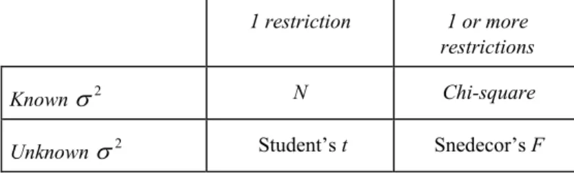
Table 4.1 shows some distributions, which are appropriate in different situations, under the assumption of normality of the disturbances.
TABLE 4.1. Some distributions used in hypothesis testing. 1 restriction 1 or more
restrictions
Known 2 N Chi-square
The statistic used for the test is built taking into account the H0 and the sample
data. In practice, as 2 is always unknown, we will use the distributions t and F. 4.1.3 Decision rule
We are going to look at two approaches for hypothesis testing: the classical approach and an alternative one based on p-values. But before seeing how to apply the decision rule, we shall examine the types of mistakes that can be made in testing hypothesis.
Types of errors in hypothesis testing
In hypothesis testing, we can make two kinds of errors: Type I error and Type II error.
Type I error
We can reject H0 when it is in fact true. This is called Type I error. Generally, we define the significance level () of a test as the probability of making a Type I error. Symbolically,
0 0
Pr(Reject H H | )
(4-5)
In other words, the significance level is the probability of rejecting H0 given that
H0 is true. Hypothesis testing rules are constructed making the probability of a Type I error fairly small. Common values for are 0.10, 0.05 and 0.01, although sometimes 0.001 is also used.
After we have made the decision of whether or not to reject H0, we have either decided correctly or we have made an error. We shall never know with certainty whether an error was made. However, we can compute the probability of making either a Type I error or a Type II error.
Type II error
We can fail to reject H0 when it is actually false. This is called Type II error.
0 1
Pr(No reject H H| )
(4-6)
In words, is the probability of not rejecting H0 given that H1 is true.
It is not possible to minimize both types of error simultaneously. In practice, what we do is select a low significance level.
Classical approach: Implementation of the decision rule
The classical approach implies the following steps:
a) Choosing . Classical hypothesis testing requires that we initially specify a
significance level for the test. When we specify a value for , we are essentially
quantifying our tolerance for a Type I error. If =0.05, then the researcher is willing to falsely reject H0 5% of the time.
b) Obtaining c, the critical value, using statistical tables. The value c is determined by .
The critical value (c) for a hypothesis test is a threshold to which the value of the test statistic in a sample is compared to determine whether or not the null hypothesis is rejected.
c) Comparing the outcome of the test statistic, s, with c, H0 is either rejected or not for a given .
The rejection region (RR), delimited by the critical value(s), is a set of values of the test statistic for which the null hypothesis is rejected. (See figure 4.1). That is, the sample space for the test statistic is partitioned into two regions; one region (the rejection region) will lead us to reject the null hypothesis H0, while the other will lead us not to reject the null hypothesis. Therefore, if the observed value of the test statistic S
is in the critical region, we conclude by rejecting H0; if it is not in the rejection region then we conclude by not rejectingH0 or failing to rejectH0.
Symbolically, 0 0 If reject If not reject s c H s c H (4-7)
If the null hypothesis is rejected with the evidence of the sample, this is a strong
conclusion. However, the acceptance of the null hypothesis is a weak conclusion because we do not know what the probability is of not rejecting the null hypothesis when it should be rejected. That is to say, we do not know the probability of making a type II error. Therefore, instead of using the expression of accepting the null hypothesis, it is more correct to say fail to reject the null hypothesis, or not reject, since what really happens is that we do not have enough empirical evidence to reject the null hypothesis.
In the process of hypothesis testing, the most subjective part is the a priori
determination of the significance level. What criteria can be used to determine it? In general, this is an arbitrary decision, though, as we have said, the 1%, 5% and 10% levels for are the most used in practice. Sometimes the testing is made conditional on several significance levels.
FIGURE 4.1. Hypothesis testing: classical approach.
An alternative approach: p-value
With the use of computers, hypothesis testing can be contemplated from a more rational perspective. Computer programs typically offer, together with the test statistic, a probability. This probability, which is called p-value (i.e., probability value), is also known as the critical or exact level of significance or the exact probability of making a
Non Rejection Region NRR Rejection Region RR c W
Type I error. More technically, the p value is defined as the lowest significance level at which a null hypothesis can be rejected.
Once the p-value has been determined, we know that the null hypothesis is rejected for any p-value, while the null hypothesis is not rejected when <p-value. Therefore, the p-value is an indicator of the level of admissibility of the null hypothesis: the higher the p-value, the more confidence we can have in the null hypothesis. The use of the p-value turns hypothesis testing around. Thus, instead of fixing a priori the significance level, the p-value is calculated to allow us to determine the significance levels of those in which the null hypothesis is rejected.
In the following sections, we will see the use of p value in hypothesis testing put into practice.
4.2 Testing hypotheses using the t test
4.2.1 Test of a single parameter
The t test
Under the CLM assumptions 1 through 9,
ˆ ~ , var( ) ˆ 1, 2,3, , j N j j j k (4-8) If we typify
ˆ ˆ ~ 0,1 1, 2,3, , ˆ ˆ ( ) var( ) j j j j j j N j k sd (4-9)The claim for normality is usually made on the basis of the Central Limit Theorem (CLT), but this is restrictive in some cases. That is to say, normality cannot always be assumed. In any application, whether normality of u can be assumed is really an empirical matter. It is often the case that using a transformation, i.e. taking logs, yields a distribution that is closer to normality, which is easy to handle from a mathematical point of view. Large samples will allow us to drop normality without affecting the results too much.
Under the CLM assumptions 1 through 9, we obtain a Student’s t distribution ˆ ˆ ( ) j j n k j t se b b b (4-10) where k is the number of unknown parameters in the population model (k-1 slope
parameters and the intercept, 1). The expression (4-10) is important because it allows us to test a hypothesis on j.
If we compare (4-10) with (4-9), we see that the Student’s t distribution derives from the fact that the parameter in sd( )ˆj has been replaced by its estimator ˆ, which is a random variable. Thus, the degrees of freedom of t are n-1-k corresponding to the degrees of freedom used in the estimation of ˆ2.
When the degrees of freedom (df) in the t distribution are large, the t
distribution approaches the standard normal distribution. In figure 4.2, the density function for normal and t distributions for different df are represented. As can be seen,
the t densi densi estim more norm the t hypo large restri when distri indep accou to te and i ˆ j . I t density fu ity function ity. In fact, mated becau e than the n mal distribut Therefor Thus, wh t distributio othesis, if th e sizes the iction, even n the df ar ibution. FIGURE Consider Since j pendent var unted for, xj st H0:j is expressed In order In a given s unctions are n, but as d , what happ use it is un normal one. tion because re, the follow
hen the num on converge he sample si normal dis n when you re larger th E 4.2. Density r the null hy j measures riables, H0 xj has no effe 0 , against d as to test H0 sample ˆj w e flatter (pl df increases pens is that nknown. Gi However, e the uncert wing conve n t mber of deg es towards ize grows, s stribution c u do not kn han 120, w y functions: n ypothesis, the partial :j 0 me fect on y. Th t any altern :j 0, it will never b latycurtic) s, t density t the t distri iven this un as the df gr tainty of not ergence in d (0 n N grees of free a distributi so will the d can be used now the pop we can take normal and t 0: j 0 H effect of x eans that, on his is called native, is ca ˆ ˆ ˆ ( ) j j j t se is natural t be exactly z
and the tai y functions ibution take ncertainty, rows the t-d t knowing distribution 0,1) edom of a S ion N(0.1). degrees of fr d to test h pulation va e the critica for different 0 xj on y aft nce x2, x3, … a significan lled the t s ) o look at ou ero, but a sm
ils are wide are closer es into acco the t distri distribution 2 decrease should be k Student’s t t In the con reedom. Th ypothesis w ariance. As al values fr degrees of fr er controlli …,xj 1, xj+1,
nce test. The
tatistic or t
ur unbiased mall value w
der than nor to the nor ount that ibution exte is nearer to es. kept in mind ( tends to inf ntext of test his means th with one u a practical from the no reedom.
ing for all ,…, xk have e statistic w the t ratio o d estimator will indicat rmal rmal 2 is ends o the d: (4-11) finity, ting a hat for unique rule, ormal other e been we use of ˆj of j, te that
the null hypothesis could be true, whereas a large value will indicate a false null hypothesis. The question is: how far is ˆj from zero?
We must recognize that there is a sampling error in our estimate ˆj, and thus the size of ˆj must be weighted against its sampling error. This is precisely what we do when we use ˆ
j
t , since this statistic measures how many standard errors ˆj is away from zero. In order to determine a rule for rejecting H0, we need to decide on the relevant alternative hypothesis. There are three possibilities: one-tail alternative hypotheses (right and left tail), and two-tail alternative hypothesis.
One-tail alternative hypothesis: right
First, let us consider the null hypothesis
0: j 0
H
against the alternative hypothesis
1: j 0
H
This is a positivesignificance test. In this case, the decision rule is the following:
Decision rule ˆ 0 ˆ 0 If reject If not reject j j n k n k t t H t t H (4-12)
Therefore, we reject H0:j 0 in favor of H1:j 0 at when ˆ
j n k
t t as can be seen in figure 4.3. It is very clear that to reject H0 against H1:j 0, we must get a positive ˆ
j
t . A negative ˆ
j
t , no matter how large, provides no evidence in favor of
1: j 0
H . On the other hand, in order to obtain tn k
in the t statistical table, we only
need the significance level and the degrees of freedom.
It is important to remark that as decreases, tn k increases.
To a certain extent, the classical approach is somewhat arbitrary, since we need to choose in advance, and eventually H0 is either rejected or not.
In figure 4.4, the alternative approach is represented. As can be seen by observing the figure, the determination of the p-value is the inverse operation to find the value of the statistical tables for a given significance level. Once the p-value has been determined, we know that H0 is rejected for any level of significance of >p-value, while the null hypothesis is not rejected when <p-value.
FIG EXAM linear in the we mu admis becau observ or 0.2 0.05 40 t corres not co =1.17 reject URE 4.3. Reje alter MPLE 4.1 Is the As seen in r model, is equ model ust test wheth
With a ran The numb The quest ssible? Next, w 1) In this c 2) The test 3) Decisio It is usefu use the valueo vations minus 20, in statistica As t<1.30 1.684 ) or sponds to =0 onsistent with In the alte 71 for a t with ed. ection region rnative hypot e marginal pr n example 1.1 uivalent to tes her ndom sample o ers in parenth tion we pose we answer thi case, the null
t statistic is: on rule ul to use seve of t is relativel s 2 estimated p al tables with 03, we do no =0.01 ( 0.01 40 t 0.10. Therefor Keynes’s pro ernative appro h 40 df is equ using t: righ thesis. ropensity to co , testing the 3 sting whether cons of 42 observat i cons heses, below th e is the follo s question. and alternativ 0 1 1 1 ˆ ˆ ( ) t se eral significan ly small (smal parameters). I one tail, or tw ot reject H0 f 2.423 ), as c re, we cannot oposition 3. oach, as can ual to 0.124. F ht-tail FIGU onsume smal 3rd propositio the intercept i 1 2 s in 1 0 ations, the follo
(0.350)0.41 0.8(0.0 = + he estimates, a owing: is the ve hypotheses 0 1 1 1 : 0 : 0 H H 0 1 1 ˆ 0 0 ˆ 0 ( ) se nce levels. L ller than 1.5). If we look at t wo tails, respec for =0.10, a can been in f t reject H0 in be seen in fi For <0.124 URE 4.4. p-valu ller than the a
on of the Keyn is significativ nc u owing results 62) 843inci are standard e e third propo are the follow
0.41 1.171 0.35 et us begin w In this case, t the t statistica ctively), we fi and therefore figure 4.5. In favor H1. In figure 4.6, the - for example ue using t: rig hypothesis. average prope nesian consum e1y greater th have been ob errors (se) of th osition of the wing: with a signific the degrees of al table (row 4 nd 0.10 40 1.30 t we cannot r this figure, t other words, e p-value corr e, 0.10, 0.05 a ght-tail altern ensity to consu mption functio han 0. That is btained he estimators. e Keynesian cance level o f freedom are 40 and column 03 reject for = the rejection the sample da responding to and 0.01-, H0 native ume? on in a to say, . theory of 0.10 40 (42 n 0.10, =0.05 ( region ata are o a 1 ˆ t is not
FIGU t One-again D ˆ j t 1: H provi deter while URE 4.5. Exam t with a right--tail alterna Consider nst the altern This is a In this ca Decision rul Therefor n t , as ca 0 j , we ides no evid In figure rmined, we e the null hy mple 4.1: Reje -tail alternati ative hypoth r now the nu native hypo a negativesi
ase, the dec
le I I re, we reje an be seen e must get dence in fav e 4.8 the alt know that ypothesis is ection region ive hypothesi hesis: left ull hypothe othesis ignificance ision rule is ˆ ˆ If If j j t t ct H0:j n in figure a negative vor of H1: ternative ap t H0 is rejec s not rejecte using is. FIG sis 0: j 0 H 1: j 0 H test. s the follow re n n k n k t t 0 in favo 4.7. It is ˆ j t . A po 0 j . pproach is r cted for an ed when <p GURE 4.6. Exa right-tail 0 0 wing: eject not reject H H or of H1: very clear ositive ˆ j t , epresented. ny level of p-value. mple 4.1: p-v alternative h 0 0 H H 0 j at a r that to re no matter Once the p significanc value using t w hypothesis. ( a given eject H0 ag how large p-valuehas ce of >p-v with (4-13) when gainst it is, been value,
FIG EXAM birth where in per W T morta 0.01 130 1 t There of chi of mo 5% an 2.966 FIGU Two-Reje Re R GURE 4.7. Rej alter MPLE 4.2 Has The follo s (deathun5). e gnipc is the rcentage. With a sample o The numbers in One of the ality. To answ The null a Since the 0.01 2 t60 2.39
efore, the gros ildren under 5 ortality of chil nd 10%. In the alte for a t with 6 URE 4.9. Exam t with a left-t -tail alterna Consider Non Rejection Region NRR ection egion RR n k t jection region rnative hypot income a neg wing model h gross national of 130 countri deathu n parentheses e questions po er this questio and alternative 0 2 1 2 : 0 : 0 H H t value is r 90 . Given th ss national inc .That is to say ldren under 5. ernative appro 61 df is equal t mple 4.2: Reje tail alternativ ative hypoth r now the nu 0 n using t: left-thesis. gative influenc
has been used 5 deathun l income per c ies (workfile h (5.93) 5i 27.91 un = -, below the es osed by resear on, the followi e hypotheses, a 0
0
relatively hig at t<-2.390, a come per capit
y, the higher th . As H0 has be oach, as can b to 0.0000. For ection region ve hypothesis hesis ull hypothe n k t -tail FIGU ce on infant m to explain the 1 2gnipc capita and ilitr hdr2010), the (0.00028) 0.000826gn -stimates, are s rchers is whet ing hypothesi and the test st
2 2 ˆ ˆ ( ) t se gh, let us sta as is shown ta has an influ he gross natio een rejected f be seen in figu r all >0.0000 using s. F IGU sis 0: j 0 H No α p-val URE 4.8. p-val mortality? e deaths of chi 3ilitrate u
rate is the adu following est (0.183) 2.043 i nipc + i tandard errors ther income h s testing is car tatistic, are the 0.000826 0.00028 art testing wi in figure 4.9 uence that is s onal income pe for =0.01, it ure 4.10, the p 0, such as 0.01 RE 4.10. Exam left-tail a 0 on rejected for >p-value Rejecte for ɑ<p-val lue ˆj t lue using t: le hypothesis. ildren under 5 ult (% 15 and imation has b i ilitrate s (se) of the es has a negative rried out: e following: 6 2.966 th a level of , we reject H significantly n er capita the lo will also be re p-value corre 1, 0.05 and 0.1 mple 4.2: p-v alternative hy ed lue 0 eft-tail altern 5 years per 100 older) illitera een obtained: stimators. e influence on f 1%. For H0 in favour negative in mo ower the perc rejected for lev esponding to a 10, H0 is rejec value using t w ypothesis. n k t ative 00 live cy rate n infant =0.01, of H1. ortality centage vels of a 1 ˆ t =-cted. with a
again theor abso D as ca must In while rejec symm FIG two-that “ EXAM where the ar and h outcom error” nst the altern This is t ry or comm lute value o In this ca Decision rul Therefor an be seen i t obtain a la It is imp n the altern e H0 is rejec cted when metrical wa GURE 4.11. Rej alter When a sided hypot “xj is statist MPLE 4.3 Has t To explain e rooms is the rea and crime
The outpu has been taken
me to perform ”; and “Prob” native hypo the relevant mon sense. of the t stati ase, the dec
le re, we rejec in figure 4. arge enough ortant to rem native appro cted for any
<p-value. I ay, as is show jection region rnative hypot specific alte thesis testin tically signif the rate of cri
n housing pric
pri
number of ro is crimes com ut for the fitted n from E-view m a significanc is the p-value othesis t alternative When the stic. This is ision rule is ˆ ˆ If If j j t t ct H0:j 11. In this c ˆ j t which i mark that as oach, once y level of sig In this case wn in figure n using t: two thesis. ernative hyp ng. If H0 is r ficant at the
ime play a rol
ces in an Amer
1 2
ice ro
ooms of the ho mmitted per cap
d model, using ws. The mean ce test, that is to perform a 1: j 0 H e when the alternative s a significa s the follow /2 /2 rej no n k n k t t 0 in favor case, in ord s either pos s decreas the p-valu gnificance o , the p-valu e 4.12. o-tail FIGU pothesis is n rejected in f e level ”. le in the price rican town, th 3 oomslows ouse, lowstat i apita in the are g the file hpri
ning of the fi to say, it is th two-tailed tes 0 e sign of j is two-side nce test. wing: 0 0 ject ot reject H H of H1:j der to reject sitive or neg es, /2 n k t incr e has been of >p-valu ue is distribu URE 4.12. p-va not stated, i favor of H1 e of houses in he following m 4 stat crime is the percenta ea. ce2 (first 55 o irst three colu he ratio betwe st. is not wel ed, we are 0 0 at wh t H0 against gative. reases in ab determined ue, the null h uted betwee alue using t: tw hypothesis. t is usually at a given an area? model is estim e u age of people observations), umns is clear een the “Coeff
ll determine interested i ( when ˆ j t t H1:j 0 bsolute value d, we know hypothesis en both tail wo-tail altern considered , we usuall mated: of “lower sta appears in tab : “t-Statistic” ficient” and th ed by in the (4-14) /2 n k t , 0, we e. w that is not s in a native to be ly say atus” in ble 4.2 is the he “Std
role in 0.01/ 2 51 t above on ho the p-greate the p-reject param wher from EXAM In relation n the price of To answer In this cas TABLE 4 C ROOMS LOWST CRIME Since the 0.01/ 2 50 2.69 t e 20). Given th using prices f In the alte
-valuefor the er than 4.016
-value, as sho ed for all sign
FIGURE So far w meter takes re the param Thus, the As befor m the hypoth MPLE 4.4 Is the To answer n to this mode houses in that r this question se, the null and
0 4 1 4 : : H H 4.2. Standard Variable S TAT t value is re 9 . (In the usu hat t 2.69, for a significan ernative appro coefficient o is 0.0001 and own in Figure nificance level 4.13. Examp we have se s the value meter in H0 t e appropriat re, ˆ j t mea hesized valu e elasticity exp r these questio ln(fruit)
el, the researc t area. n, the followin d alternative h 0 0 d output in th Coeffic -1569 6788 -268.1 -3853 elatively high ual statistical t we reject H0 nce level of 1% ach, we can p f crime is 0.0 d the probabil 4.13, is distr ls greater than le 4.3: p-valu een signific 0 in H0. N takes any va H te t statistic t asures how ue of 0 j . xpenditure in f ons, we are go 1 2 ) ln(i cher questions ng procedure h hypothesis and 4 ˆ ( t se he regression cient Std. E 93.61 80 8.401 12 1636 80 .564 95 h, let us by s tables for t di in favour of H % and, thus, o perform the te 0002. That me lity of t being ributed in the n 0.0002, such ue using t with cant tests o Now we are alue: 0: j j H c is ˆ ˆ ˆ ( ) j j j j t se many estim fruit/income
oing to use the
3
)
inc house
s whether the has been carrie d the test statis
4 4 3854 ˆ ) 960 explaining ho Error t-St 021.989 -10.720 0.70678 -9.5618 -tart testing w istribution, th H1. Therefore, of 5% and 10% st with more p eans that the p g smaller than two tails. As h as 0.01, 0.05 h a two-tail a of one-tail going to lo 0 j 0 ) j mated stand equal to 1? Is e following mo 4 ehsize pun rate of crime ed out. stic are the fol
4.016 ouse price. n= tatistic P 1.956324 5.606910 3.322690 4.015962 with a level o ere is no info crime has a s %. precision. In t probability of -4.016 is 0.0 can be seen and 0.10. lternative hy and two-ta ook at a mo dard deviati s fruit a luxur
odel for the ex
nders u e in an area p llowing: =55. Prob. 0.0559 0.0000 0.0017 0.0002 of 1%. For ormation for e significant inf table 4.2 we s f the t statistic 0001. That is in this figure ypothesis. ails, in wh more general ions ˆj is ry good? xpenditure in f plays a =0.01, each df fluence ee that c being to say, e, H0 is hich a l case away fruit:
where inc is disposable income of household, househsize is the number of household members and punder5 is the proportion of children under five in the household.
As the variables fruit and inc appear expressed in natural logarithms, then 2 is the expenditure
in fruit/income elasticity. Using a sample of 40 households (workfile demand), the results of table 4.3 have been obtained.
TABLE 4.3. Standard output in a regression explaining expenditure in fruit. n=40.
Variable Coefficient Std. Error t-Statistic Prob.
C -9.767654 3.701469 -2.638859 0.0122
LN(INC) 2.004539 0.512370 3.912286 0.0004
HOUSEHSIZE -1.205348 0.178646 -6.747147 0.0000
PUNDER5 -0.017946 0.013022 -1.378128 0.1767
Is the expenditure in fruit/income elasticity equal to 1?
To answer this question, the following procedure has been carried out:
In this case, the null and alternative hypothesis and the test statistic are the following:
0 2 1 2 : 1 : 1 H H 0 2 2 2 2 2 ˆ ˆ 1 2.005 1 1.961 ˆ ˆ 0.512 ( ) ( ) t se se
For =0.10, we find that 0.10/ 2 0.10/ 2
36 35 1.69
t t . As | |t >1.69, we reject H0. For =0.05,
0.05/ 2 0.05/ 2
36 35 2.03
t t . As | |t <2.03, we do not reject H0 for =0.05, nor for =0.01. Therefore, we reject
that the expenditure on fruit/income elasticity is equal to 1 for =0.10, but we cannot reject it for =0.05, nor for =0.01.
Is fruit a luxury good?
According to economic theory, a commodity is a luxury good when its expenditure elasticity with respect to income is higher than 1. Therefore, to answer to the second question, and taking into account that the t statistic is the same, the following procedure has been carried out:
0: 2 1
H H1:2 1.
For =0.10, we find that 0.10 0.10
36 35 1.31
t t . As t>1.31, we reject H0 in favour of H1. For =0.05,
0.05 0.05
36 35 1.69
t t . As t>1.69, we reject H0 in favour of H1. For =0.01, t360.01t350.012.44. As t<2.44, we
do not reject H0. Therefore, fruit is a luxury good for =0.10 and =0.05, but we cannot reject H0 in
favour of H1 for =0.01.
EXAMPLE 4.5 Is the Madrid stock exchange market efficient?
Before answering this question, we will examine some previous concepts. The rate of return of an asset over a period of time is defined as the percentage change in the value invested in the asset during that period of time. Let us now consider a specific asset: a share of an industrial company acquired in a Spanish stock market at the end of one year and remains until the end of next year. Those two moments of time will be denoted by t-1 and t respectively. The rate of return of this action within that year can be expressed by the following relationship:
1 t t t t t P D A RA P -D + + (4-15)
where Pt: is the share price at the end of period t, Dt: are the dividends received by the share during the period t, and At: is the value of the rights that eventually corresponded to the share during the period t
Thus, the numerator of (4-15) summarizes the three types of capital gains that have been received for the maintenance of a share in year t; that is to say, an increase or decrease in quotation, dividends and rights on capital increase. Dividing by Pt-1, we obtain the rate of profit on share value at the end of the previous period. Of these three components, the most important one is the increase in quotation. Considering only that component, the yield rate of the action can be expressed by
1 1 t t t P RA P -D (4-16)
or, alternatively if we use a relative rate of variation, by 2t ln t
RA D P (4-17)
In the same way as Rat represents the rate of return of a particular share in either of the two expressions, we can also calculate the rate of return of all shares listed in the stock exchange. The latter rate of return, which will be denoted by RMt, is called the market rate of return.
So far we have considered the rate of return in a year, but we can also apply expressions such as (4-16), or (4-17), to obtain daily rates of return. It is interesting to know whether the rates of return in the past are useful for predicting rates of return in the future. This question is related to the concept of market efficiency. A market is efficient if prices incorporate all available information, so there is no possibility of making abnormal profits by using this information.
In order to test the efficiency of a market, we define the following model, using daily rates of return defined by (4-16):
1 2 1
92 92t t t
rmad rmad u (4-18)
If a market is efficient, then the parameter 2 of the previous model must be 0. Let us now
compare whether the Madrid Stock Exchange is efficient as a whole.
The model (4-18) has been estimated with daily data from the Madrid Stock Exchange for 1992, using file bolmadef. The results obtained are the following:
1 (0.0007) (0.0629) 92t 0.0004 0.1267 92t rmad + rmad -R2=0.0163 n=247
The results are paradoxical. On the one hand, the coefficient of determination is very low (0.0163), which means that only 1.63% of the total variance of the rate of return is explained by the previous day’s rate of return. On the other hand, the coefficient corresponding to the rate of significance of the previous day is statistically significant at a level of 5% but not at a level of 1% given that the t statistic is equal to 0.1267/0.0629=2.02, which is slightly larger in absolute value than t2450.01t600.01=2.00. The reason for this apparent paradox is that the sample size is very high. Thus, although the impact of the explanatory variable on the endogenous variable is relatively small (as indicated by the coefficient of determination), this finding is significant (as evidenced by the statistical t) because the sample is sufficiently large.
To answer the question as to whether the Madrid Stock Exchange is an efficient market, we can say that it is not entirely efficient. However, this response should be qualified. In financial economics there is a dependency relationship of the rate of return of one day with respect to the rate corresponding to the previous day. This relationship is not very strong, although it is statistically significant in many world stock markets due to market frictions. In any case, market players cannot exploit this phenomenon, and thus the market is not inefficient, according to the above definition of the concept of efficiency.
EXAMPLE 4.6 Is the rate of return of the Madrid Stock Exchange affected by the rate of return of the Tokyo Stock Exchange?
The study of the relationship between different stock markets (NYSE, Tokyo Stock Exchange Madrid Stock Exchange, London Stock Exchange, etc.) has received much attention in recent years due to the greater freedom in the movement of capital and the use of foreign markets to reduce the risk in portfolio management. This is because the absence of perfect market integration allows diversification of risk. In any case, there is a world trend toward a greater global integration of financial markets in general and stock markets in particular.
If markets are efficient, and we have seen in example 4.5 that they are, the innovations (new information) will be reflected in the different markets for a period of 24 hours.
It is important to distinguish between two types of innovations: a) global innovations, which is news generated around the world and has an influence on stock prices in all markets, b) specific innovations, which is the information generated during a 24 hour period and only affects the price of a particular market. Thus, information on the evolution of oil prices can be considered as a global innovation, while a new financial sector regulation in a country would be considered a specific innovation.
According to the above discussion, stock prices quoted at a session of a particular stock market are affected by the global innovations of a different market which had closed earlier. Thus, global innovations included in the Tokyo market will influence the market prices of Madrid on the same day.
The following model shows the transmission of effects between the Tokyo Stock Exchange and the Madrid Stock Exchange in 1992:
rmad92t =1+2rtok92t+ut (4-19) where rmad92t is the rate of return of the Madrid Stock Exchange in period t and rtok92t is the rate of return of the Tokyo Stock Exchange in period t. The rates of return have been calculated according to (4-16).
In the working file madtok you can find general indices of the Madrid Stock Exchange and the Tokyo Stock Exchange during the days both exchanges were open simultaneously in 1992. That is, we eliminated observations for those days when any one of the two stock exchanges was closed. In total, the number of observations is 234, compared to the 247 and 246 days that the Madrid and Tokyo Stock Exchanges were open.
The estimation of the model (4-19) is as follows:
(0.0007) (0.0375)
92t 0.0005 0.1244 92t rmad + rtok
R2=0.0452 n=235
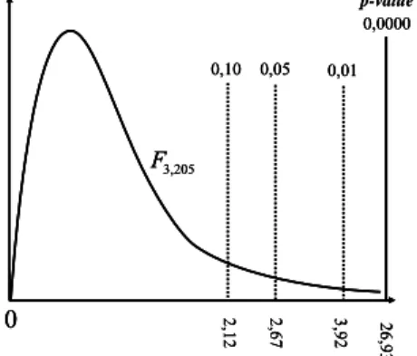
Note that the coefficient of determination is relatively low. However, for testing H0:2=0, the
statistic t = (0.1244/0.0375) = 3.32, which implies that we reject the hypothesis that the rate of return of the Tokyo Stock Exchange has no effect on the rate of return of the Madrid Stock Exchange, for a significance level of 0.01.
Once again we find the same apparent paradox which appeared when we analyzed the efficiency of the Madrid Stock Exchange in example 4.5 except for one difference. In the latter case, the rate of return from the previous day appeared as significant due to problems arising in the elaboration of the general index of the Madrid Stock Exchange.
Consequently, the fact that the null hypothesis is rejected implies that there is empirical evidence supporting the theory that global innovations from the Tokyo Stock Exchange are transmitted to the quotes of the Madrid Stock Exchange that day.
4.2.2 Confidence intervals
Under the CLM, we can easily construct a confidence interval (CI) for the population parameter, j. CI are also called interval estimates because they provide a range of likely values for j, and not just a point estimate.
The CI is built in such a way that the unknown parameter is contained within the range of the CI with a previously specified probability.
By using the fact that
ˆ ˆ ( ) j j n k j t se b b b - /2 ˆ /2 Pr ˆ 1 ( ) j j n k n k j t t se
Operating to put the unknownj alone in the middle of the interval, we have
/2 /2
ˆ ˆ ˆ ˆ
Prjse( )j tn k j jse( )j tn k 1
Therefore, the lower and upper bounds of a (1-) CI respectively are given by
/2 ˆ ( )ˆ j j se j tn k /2 ˆ ( )ˆ j j se j tn k
If random samples were obtained over and over again with j, and j computed each time, then the (unknown) population value would lie in the interval (j,
j
) for (1 )% of the samples. Unfortunately, for the single sample that we use to construct CI, we do not know whether jis actually contained in the interval.
Once a CI is constructed, it is easy to carry out two-tailed hypothesis tests. If the null hypothesis is H0:j aj, then H0 is rejected against H1:j aj at (say) the 5% significance level if, and only if, ajis not in the 95% CI.
To illustrate this matter, in figure 4.14 we constructed confidence intervals of 90%, 95% and 99%, for the marginal propensity to consumption -2- corresponding to example 4.1.
FIGURE 4.14. Confidence intervals for marginal propensity to consume in example 4.1. 4.2.3 Testing hypotheses about a single linear combination of the parameters
In many applications we are interested in testing a hypothesis involving more than one of the population parameters. We can also use the t statistic to test a single linear combination of the parameters, where two or more parameters are involved.
There are two different procedures to perform the test with a single linear combination of parameters. In the first, the standard error of the linear combination of parameters corresponding to the null hypothesis is calculated using information on the covariance matrix of the estimators. In the second, the model is reparameterized by introducing a new parameter derived from the null hypothesis and the reparameterized model is then estimated; testing for the new parameter indicates whether the null hypothesis is rejected or not. The following example illustrates both procedures.
EXAMPLE 4.7 Are there constant returns to scale in the chemical industry?
To examine whether there are constant returns to scale in the chemical sector, we are going to use the Cobb-Douglas production function, given by
1 2 3
ln(output) ln(labor) ln(capital)u (4-20) In the above model parameters 2 and 3 are elasticities (output/labor and output/capital).
Before making inferences, remember that returns to scale refers to a technical property of the production function examining changes in output subsequent to a change of the same proportion in all inputs, which are labor and capital in this case. If output increases by that same proportional change then there are constant returns to scale. Constant returns to scale imply that if the factors labor and capital increase at a certain rate (say 10%), output will increase at the same rate (e.g., 10%). If output increases by more than that proportion, there are increasing returns to scale. If output increases by less than that proportional change, there are decreasing returns to scale. In the above model, the following occurs
- if 2+3=1, there are constant returns to scale.
- if 2+3>1, there are increasing returns to scale.
- if 2+3<1, there are decreasing returns to scale.
0,90 0,95 0,99 0. 73 9 0. 94 7 0. 71 8 0. 67 5 0. 96 8 1. 01 1 0. 84 3
Data used for this example are a sample of 27 companies of the primary metal sector (workfile prodmet), where output is gross value added, labor is a measure of labor input, and capital is the gross value of plant and equipment. Further details on construction of the data are given in Aigner, et al. (1977) and in Hildebrand and Liu (1957); these data were used by Greene in 1991. The results obtained in the estimation of model (4-20), using any econometric software available, appear in table 4.4.
TABLE 4.4. Standard output of the estimation of the production function:
model (4-20).
Variable Coefficient Std. Error t-Statistic Prob. constant 1.170644 0.326782 3.582339 0.0015 ln(labor) 0.602999 0.125954 4.787457 0.0001 ln(capital) 0.375710 0.085346 4.402204 0.0002 To answer the question posed in this example, we must test
0: 2 3 1
H against the following alternative hypothesis
1: 2 3 1
H
According to H0, it is stated that 23 1 0. Therefore, the t statistic must now be based on
whether the estimated sum ˆ2ˆ31 is sufficiently different from 0 to reject H0 in favor of H1.
Two procedures will be used to test this hypothesis. In the first, the covariance matrix of the estimators is used. In the second, the model is reparameterized by introducing a new parameter.
Procedure: using covariance matrix of estimators
According to H0, it is stated that 23 1 0. Therefore, the t statistic must now be based on whether the estimated sum ˆ2ˆ31 is sufficiently different from 0 to reject H0 in favor of H1. To
account for the sampling error in our estimators, we standardize this sum by dividing by its standard error: 2 3 2 3 ˆ ˆ 2 3 ˆ ˆ 1 ˆ ˆ ( ) t se Therefore, if 2 3 ˆ ˆ
t is large enough, we will conclude, in a two side alternative test, that there are not constant returns to scale. On the other hand, if
2 3
ˆ ˆ
t is positive and large enough, we will reject, in a one side alternative test (right), H0 in favour of H1:23 1. Therefore, there are increasing returns to
scale.
On the other hand , we have
2 3 2 3 ˆ ˆ ˆ ˆ ( ) var( ) se where 2 3 2 3 2 3 ˆ ˆ ˆ ˆ ˆ ˆ
var( ) var( ) var( ) 2 covar( , )
Hence, to compute se(ˆ2ˆ3) you need information on the estimated covariance of estimators. Many econometric software packages (such as e-views) have an option to display estimates of the covariance matrix of the estimator vector ’. In this case, the covariance matrix obtained appears in table 4.5. Using this information, we have
2 3 ˆ ˆ ( ) 0.015864 0.007284 2 0.009616 0.0626 se 2 3 2 3 ˆ ˆ 2 3 ˆ ˆ 1 0.02129 0.3402 ˆ ˆ 0.0626 ( ) t se
TABLE 4.5. Covariance matrix in the production function. constant ln(labor) ln(capital) constant 0.106786 -0.019835 0.001189 ln(labor)) -0.019835 0.015864 -0.009616 ln(capital) 0.001189 -0.009616 0.007284
Given that t=0.3402, it is clear that we cannot reject the existence of constant returns to scale for the usual significance levels. Given that the t statistic is negative, it makes no sense to test whether there areincreasing returns to scale
Procedure: reparameterizing the model by introducing a new parameter
It is easier to perform the test if we apply the second procedure. A different model is estimated in this procedure, which directly provides the standard error of interest. Thus, let us define:
2 3 1
thus, the null hypothesis that there are constant returns to scale is equivalent to saying that H0:0. From the definition of we have 2 31. Substituting 2 in the original equation:
1 3 3
ln(output) ( 1) ln(labor) ln(capital)u
Hence,
1 3
ln(output labor/ ) ln(labor) ln(capital labor/ )u
Therefore, to test whether there are constant returns to scale is equivalent to carrying out a significance test on the coefficient of ln(labor) in the previous model. The strategy of rewriting the model so that it contains the parameter of interest works in all cases and is usually easy to implement. If we apply this transformation to this example, we obtain the results of Table 4.6.
As can be seen we obtain the same result:
ˆ ˆ 0.3402 ˆ ( ) t se
TABLE 4.6. Estimation output for the production function: reparameterized model.
Variable Coefficient Std. Error t-Statistic Prob. constant 1.170644 0.326782 3.582339 0.0015 ln(labor) -0.021290 0.062577 -0.340227 0.7366 ln(capital/labor) 0.375710 0.085346 4.402204 0.0002
EXAMPLE 4.8 Advertising or incentives?
The Bush Company is engaged in the sale and distribution of gifts imported from the Near East. The most popular item in the catalog is the Guantanamo bracelet, which has some relaxing properties. The sales agents receive a commission of 30% of total sales amount. In order to increase sales without expanding the sales network, the company established special incentives for those agents who exceeded a sales target during the last year.
Advertising spots were radio broadcasted in different areas to strengthen the promotion of sales. In those spots special emphasis was placed on highlighting the well-being of wearing a Guantanamo bracelet.
The manager of the Bush Company wonders whether a dollar spent on special incentives has a higher incidence on sales than a dollar spent on advertising. To answer that question, the company's econometrician suggests the following model to explain sales:
1 2 3
sales advertincent u
where incent are incentives to the salesmen and advert are expenditures in advertising. The variables sales, incent and advert are expressed in thousands of dollars.
Using a sample of 18 sale areas (workfile advincen), we have obtained the output and the covariance matrix of the coefficients that appear in table 4.7 and in table 4.8 respectively.
TABLE 4.7. Standard output of the regression for example 4.8.
Variable Coefficient Std. Error t-Statistic Prob.
constant 396.5945 3548.111 0.111776 0.9125 advert 18.63673 8.924339 2.088304 0.0542
incent 30.69686 3.604420 8.516448 0.0000
TABLE 4.8. Covariance matrix for example 4.8.
C ADVERT INCENT
constant 12589095 -26674 -7101 advert -26674 79.644 2.941
incent -7101 2.941 12.992
In this model, the coefficient 2 indicates the increase in sales produced by a dollar increase in
spending on advertising, while3 indicates the increase caused by a dollar increase in the special
incentives, holding fixed in both cases the other regressor.
To answer the question posed in this example, the null and the alternative hypothesis are the following: 0 3 2 1 3 2 : 0 : 0 H H
The t statistic is built using information about the covariance matrix of the estimators:
3 2 3 2 ˆ ˆ 3 2 ˆ ˆ ˆ ˆ ( ) t se 3 2 ˆ ˆ ( ) 79.644 12.992 2 2.941 9.3142 se 3 2 3 2 ˆ ˆ 3 2 ˆ ˆ 30.697 18.637 1.295 ˆ ˆ 9.3142 ( ) t se For =0.10, we find that 0.10
15 1.341
t . As t<1.341, we do not reject H0 for =0.10, nor for
=0.05 or =0.01. Therefore, there is no empirical evidence that a dollar spent on special incentives has a higher incidence on sales than a dollar spent on advertising.
EXAMPLE4.9 Testing the hypothesis of homogeneityinthe demand for fish
In the case study in chapter 2, models for demand for dairy products have been estimated from cross-sectional data, using disposable income as an explanatory variable. However, the price of the product itself and, to a greater or lesser extent, the prices of other goods are determinants of the demand. The demand analysis based on cross sectional data has precisely the limitation that it is not possible to examine the effect of prices on demand because prices remain constant, since the data refer to the same point in time. To analyze the effect of prices it is necessary to use time series data or, alternatively, panel data. We will briefly examine some aspects of the theory of demand for a good and then move to the estimation of a demand function with time series data. As a postscript to this case, we will test one of the hypotheses which, under certain circumstances, a theoretical model must satisfy.
The demand for a commodity - say good j - can be expressed, according to an optimization process carried out by the consumer, in terms of disposable income, the price of the good and the prices of the other goods. Analytically:
1 2
( , , , , , , )
j j j m
q f p p p p di (4-21)
where
- di is the disposable income of the consumer.
- p p1, 2, , pj,pm are the prices of the goods which are taken into account by
consumers when they acquire the good j.
Logarithmic models are attractive in studies on demand,, because the coefficients are directly elasticities. The log model is given by
1 2 1 3 2 1 2
It is clear to see that all coefficients, excluding the constant term, are elasticities of different types and therefore are independent of the units of measurement for the variables. When there is no money illusion, if all prices and income grow at the same rate, the demand for a good is not affected by these changes. Thus, assuming that prices and income are multiplied by if the consumer has no money illusion, the following should be satisfied
1 2 1 2
( , , , , , , ) ( , , , , , )
j j m j j m
f lp lp lp lp lR f p p p p di (4-23) From a mathematical point of view, the above condition implies that the demand function must be homogeneous of degree 0. This condition is called the restriction of homogeneity. Applying Euler's theorem, the restriction of homogeneity in turn implies that the sum of the demand/income elasticity and of all demand/price elasticities is zero, i.e.:
1 0 j h j m q p q R h
(4-24)This restriction applied to the logarithmic model (4-22) implies that
2 3 j m 1 m 2 0
(4-25)
In practice, when estimating a demand function, the prices of many goods are not included, but only those that are closely related, either because they are complementary or substitute goods. It is also well known that the budgetary allocation of spending is carried out in several stages.
Next, the demand for fish in Spain will be studied by using a model similar to (4-22). Let us consider that in a first assignment, the consumer distributes its income between total consumption and savings. In a second stage, the consumption expenditure by function is performed taking into account the total consumption and the relevant prices in each function. Specifically, we assume that the only relevant price in the demand for fish is the price of the good (fish) and the price of the most important substitute (meat).
Given the above considerations, the following model is formulated:
1 2 3 4
ln(fish ln(fishpr) ln(meatpr) ln(cons)u (4-26) where fish is fish expenditure at constant prices, fishpr is the price of fish, meatpr is the price of meat and cons is total consumption at constant prices.
The workfile fishdem contains information about this series for the period 1964-1991. Prices are index numbers with 1986 as a base, and fish and cons are magnitudes at constant prices with 1986 as a base also. The results of estimating model (4-26) are as follows:
(2.30) (0.133) (0.112) (0.137)
ln(fish 7.788 0.460ln(- fishpr) 0.554ln(+ meatpr) 0.322ln(+ cons)
As can be seen, the signs of the elasticities are correct: the elasticity of demand is negative with respect to the price of the good, while the elasticities with respect to the price of the substitute good and total consumption are positive
In model (4-26) the homogeneity restriction implies the following null hypothesis:
2 3 4
(4-27)
To carry out this test, we will use a similar procedure to the one used in example 4.6. Now,the parameter is defined as follows
2 3 4
(4-28)
Setting 2 34, the following model has been estimated:
1 3 4
ln(fish ln(fishpr) ln(meatpr fishpr ) ln(cons fishpr )u (4-29) The results obtained were the following:
(2.30) (0.1334) (0.112) (0.137)
ln(fishi 7.788 0.4596ln(- fishpri) 0.554ln(+ meatpri) 0.322ln(+ consi)
Using (4-28), testing the null hypothesis (4-27) is equivalent to testing that the coefficient of ln(fishpr) in (4-29) is equal to 0. Since the t statistic for this coefficient is equal to -3.44 and 0.01/ 2
24
t =2.8, we reject the hypothesis of homogeneity regarding the demand for fish.
4.2.4 Economic importance versus statistical significance
Up until now we have emphasized statistical significance. However, it is important to remember that we should pay attention to the magnitude and the sign of the estimated coefficient in addition to t statistics.
Statistical significance of a variable xj is determined entirely by the size of ˆ
j
t , whereas the economic significance of a variable is related to the size (and sign) of ˆj. Too much focus on statistical significance can lead to the false conclusion that a variable is “important” for explaining y, even though its estimated effect is modest.
Therefore, even if a variable is statistically significant, you need to discuss the magnitude of the estimated coefficient to get an idea of its practical or economic importance.
4.3 Testing multiple linear restrictions using the F test.
So far, we have only considered hypotheses involving a single restriction. But frequently, we wish to test multiple hypotheses about the underlying parameters
1, , , ,2 3 k
.
In multiple linear restrictions, we will distinguish three types: exclusion restrictions, model significance and other linear restrictions.
4.3.1 Exclusion restrictions
Null and alternative hypotheses; unrestricted and restricted model
We begin with the leading case of testing whether a set of independent variables has no partial effect on the dependent variable, y. These are called exclusion restrictions. Thus, considering the model
1 2 2 3 3 4 4 5 5
y x x x x u (4-30)
the null hypothesis in a typical example of exclusion restrictions could be the following:
0: 4 5 0
H
This is an example of a set of multiple restrictions, because we are putting more than one restriction on the parameters in the above equation. A test of multiple restrictions is called a joint hypothesis test.
The alternative hypothesis can be expressed in the following way
H1: H0 is not true
It is important to remark that we test the above H0 jointly, not individually. Now, we are going to distinguish between unrestricted (UR) and restricted (R) models. The unrestricted model is the reference model or initial model. In this example the unrestricted model is the model given in (4-30). The restricted model is obtained by imposing H0 on the original model. In the above example, the restricted model is
1 2 2 3 3
y x x u
By definition, the restricted model always has fewer parameters than the unrestricted one. Moreover, it is always true that
RSSRRSSUR
where RSSR is the RSS of the restricted model, and RSSUR is the RSS of the unrestricted model. Remember that, because OLS estimates are chosen to minimize the sum of squared residuals, the RSS never decreases (and generally increases) when certain restrictions (such as dropping variables) are introduced into the model.
The increase in the RSS when the restrictions are imposed can tell us something about the likely truth of H0. If we obtain a large increase, this is evidence against H0, and this hypothesis will be rejected. If the increase is small, this is not evidence against
H0, and this hypothesis will not be rejected. The question is therefore whether the observed increase in the RSS when the restrictions are imposed is large enough, relative to the RSS in the unrestricted model, to warrant rejecting H0.
The answer depends on but we cannot carry out the test at a chosen until we have a statistic whose distribution is known, and is tabulated, under H0. Thus, we need a way to combine the information in RSSR and RSSUR to obtain a test statistic with a known distribution under H0.
Now, let us look at the general case, where the unrestricted model is
1 2 2 3 3 k k+
y x x x u (4-31)
Let us suppose that there are q exclusion restrictions to test. H0 states that q of the variables have zero coefficients. Assuming that they are the last q variables, H0 is stated as
0: k q 1 k q 2 k 0
H (4-32)
The restricted model is obtained by imposing the q restrictions of H0 on the unrestricted model.
1 2 2 3 3 k q k q+
y x x x u (4-33)
H1 is stated as
H1: H0 is not true (4-34)
Test statistic: F ratio
The F statistic, or F ratio, is defined by
( ) / / ( ) R UR UR RSS RSS q F RSS n k (4-35)
where RSSR is the RSS of the restricted model, and RSSUR is the RSS of the unrestricted model and q is the number of restrictions; that is to say, the number of equalities in the null hypothesis.
In order to use the F statistic for a hypothesis testing, we have to know its sampling distribution under H0 in order to choose the value c for a given , and determine the rejection rule. It can be shown that, under H0, and assuming the CLM
assumptions hold, the F statistic is distributed as a Snedecor’s F random variable with (q,n-k) df. We write this result as
0 q n k,