econstor Make Your Publication Visible

(1)

econ

stor

Make Your Publication Visible

zbw

Leibniz-Informationszentrum Wirtschaft

Leibniz Information Centre for Economics

Dragomirescu-Gaina, Catalin

Article

An empirical inquiry into the determinants of public

education spending in Europe

IZA Journal of European Labor Studies Provided in Cooperation with: Institute for the Study of Labor (IZA)

Suggested Citation: Dragomirescu-Gaina, Catalin (2015) : An empirical inquiry into the determinants of public education spending in Europe, IZA Journal of European Labor Studies, ISSN 2193-9012, Springer, Heidelberg, Vol. 4, Iss. 25, pp. 1-24, http://dx.doi.org/10.1186/ s40174-015-0049-7

This Version is available at: http://hdl.handle.net/10419/127464

Standard-Nutzungsbedingungen:

Die Dokumente auf EconStor dürfen zu eigenen wissenschaftlichen Zwecken und zum Privatgebrauch gespeichert und kopiert werden. Sie dürfen die Dokumente nicht für öffentliche oder kommerzielle Zwecke vervielfältigen, öffentlich ausstellen, öffentlich zugänglich machen, vertreiben oder anderweitig nutzen.

Sofern die Verfasser die Dokumente unter Open-Content-Lizenzen (insbesondere CC-Lizenzen) zur Verfügung gestellt haben sollten, gelten abweichend von diesen Nutzungsbedingungen die in der dort genannten Lizenz gewährten Nutzungsrechte.

Terms of use:

Documents in EconStor may be saved and copied for your personal and scholarly purposes.

You are not to copy documents for public or commercial purposes, to exhibit the documents publicly, to make them publicly available on the internet, or to distribute or otherwise use the documents in public.

If the documents have been made available under an Open Content Licence (especially Creative Commons Licences), you may exercise further usage rights as specified in the indicated licence.

http://creativecommons.org/licenses/by/4.0/

(2)

O R I G I N A L A R T I C L E

Open Access

An empirical inquiry into the determinants

of public education spending in Europe

Catalin Dragomirescu-Gaina

Correspondence:

catalingaina@gmail.com

Independent researcher, Romania

Abstract

This paper makes two important contributions. Firstly, it uncovers some of the main economic determinants driving the dynamics of public education spending in Europe. Drawing mainly on the insights provided by Baumol’s cost theory, the baseline specification uses unit labour costs and real GDP per capita as its main determinants. Some important institutional rigidities are also highlighted. The results confirm the fast relative increase in education costs, exposing the long-term affordability challenge of public education investment. Secondly, by including a policy objective and translating the empirical specification into a decision rule, the paper touches on some less mentioned determinants, such as policy commitment. Unfortunately, there is only weak overall evidence that public education spending would increase in response to a lack of progress in the policy objective. Finally, policy implications are discussed.

JEL:D78, H41, H52, I22

Keywords:Education spending, Baumol cost disease, Policy commitment

1 Introduction

The sustained rise in the relative cost of certain public services continues to be a major source of concern for societies and governments alike. The problem has been first observed and discussed in Baumol and Bowen (1966) and Baumol (1967), with sectors such as education and health-care being given as prominent examples. Baumol (2012) further explains that the pain experienced by a society seems to be caused mainly by the relativedynamicsof these costs rather than theirlevels(see also Wolff et al., 2014). In fact, this problem has been so pervasive across both the developed and the develop-ing world, and over the last couple of decades, that it has been commonly labeled as the (Baumol’s)‘cost disease’. Obviously, such a persistent and widespread phenomenon must have roots that go deeper than country-specific characteristics and institutional arrangements.

I start from these considerations when empirically analysing a panel dataset that spans over the 2000–2012 time period and refers to current European Union (EU) member states. In this data environment, I intend to highlight some common determi-nants driving the dynamics of public education spending and to draw insights with re-spect to their policy importance. I also focus on spendingdynamicsrather thanlevels

since this allows me to address some large heterogeneity concerns in my sample. I

© 2015 Dragomirescu-Gaina.Open AccessThis article is distributed under the terms of the Creative Commons Attribution 4.0 International License (http://creativecommons.org/licenses/by/4.0/), which permits unrestricted use, distribution, and reproduction in any medium, provided you give appropriate credit to the original author(s) and the source, provide a link to the Creative Commons license, and indicate if changes were made.

(3)

construct an empirical specification building on theoretical insights borrowed mainly from Baumol (1967)‘cost model’, but also from Bowen (1980)‘revenue theory of costs’. Using just aggregate measures of unit labour costs and income per capita, I am able to capture the sustained rise in education costs (and therefore spending), despite the iner-tia observed in classroom‘production technology’(measured by student-teacher ratios). Relevant studies employing similar approaches to model education spending can be found in Fernandez and Rogerson (2001), Gundlach et al. (2001), Archibald and Feldman (2008), Wolff et al. (2014), Chen and Moul (2014). In general, their findings largely confirm the theoretical underpinnings discussed above. In fact, the Baumol’s cost theory in particular has been an excellent workhorse for empirical investiga-tions in many closely-related areas, such as health-care, general services, and other labour-intensive activities.

The paper also touches on some less mentioned determinants of education spending that bear more with political economy considerations, such as policy commitment. Here, I discuss commitment with a focus on public education spending (at primary, secondary and tertiary levels), although extensions to other policy areas (e.g., employ-ment and social security) remain possible within the same methodological approach. The understanding is that, beyond theoretical determinants and inherent institutional rigidities, there will always be some degree of policy discretion (as opposed to time-consistent policy rules that define commitment) that would amend funding allocations due to some specific considerations. As a prerequisite to evaluating policy commit-ment, I expand my empirical specification to include a policy-relevant education object-ive and attempt to establish a link between the progress registered in this objectobject-ive and the dynamics of spending (which I take to be the policy instrument). Lisbon strategy (or Europe 2010) together with its current, more detailed, Europe 2020 version were designed to promote education attainment and social cohesion, raise employment and foster innovation along with other long-term policy objectives.1Hence, I draw on these two policy agendas in search of some well-defined, consistent indicators to serve as pol-icy objectives for my analysis. With respect to education, there is only one clear and measureable policy objective mentioned in both strategies: reducing the share of early school leavers (henceforth ESL), i.e., 18–24 year-olds with less than upper secondary educational attainment who are no longer in education or training —according to the definition of the European Commission.2In this context, I investigate whether EU gov-ernments have shown determination in their pursuit for better education goals, i.e., lower ESL shares; for a positive characterization of policy commitment, I expect public education spending to increase whenever there is a lack of or insufficient progress with respect to the ESL policy objective.3

The paper makes at least two important contributions. Firstly, it empirically identifies some of the main common determinants driving the dynamics of public education spending in Europe, building on some well-established economic theories. The paper provides clear evidence that the annual growth rate in public education spending (espe-cially at primary and secondary levels) has considerably exceeded the annual growth rate in unit labour costs—a preferred measure for portraying the Baumol‘cost disease’ and an indicator of general price trends. Unfortunately, this finding also exposes the long-term affordability challenge of public education investment. A system of seemingly unrelated regression equations is proposed to account for any possible substitutions or

(4)

complementarities between different education levels. Moreover, by broadening the perspective, I show that the dynamics of total government spendingper capitacan also be easily described by relying on the same major determinants as in the case of educa-tion spending per student(a recent empirical review on public spending determinants can be found in Shelton, 2007). In addition, the paper highlights some dimensions where institutional rigidities are higher and can, therefore, generate highly persistent dynamics in public education spending (e.g., student-teacher ratio, spending share of teachers’wages).

Secondly, the paper attempts to empirically evaluate the link between education spending and education attainment, where the latter is defined in terms ofearly school leavers—a highly relevant policy objective according to the strategies promoted by the EU. In establishing such a link between the two elements, the analysis touches on the issue of policy commitment to education. Commitment here implies a very clear se-quencing of the decision-making process: spending is adjusted or decided with respect to previous/past realized performances in the policy objective. Unfortunately, I am not able to find sufficiently strong evidence that policy commitment has been a major determinant of education spending across EU states, although this finding is clearly dependent on the specific approach adopted here.

This analysis also has implications for other closely-related strands of research. On the one hand, education is known to foster technical progress and productivity growth that, in turn, provide not only resources to fund more education but also the right incentives to inspire better education choices for the young generations.4The possibility of such a virtu-ous circle highlights the importance of education investment due to its favourable conse-quences on several socio-economic dimensions, including better career prospects, faster transition from school to work, and higher social mobility. On the other hand, education usually represents a small allocation in total government spending, much smaller than other, more pressing, policy objectives such as employment and social security. In fact, short-term political considerations might dominate the public budgeting process today, especially given the high and persistent unemployment levels in Europe. However, if edu-cation costs were to continue rising faster than general prices, the governments would be forced into a difficult trade-off between the long-term affordability and provision of public education and the short-term political considerations arising from more pressing objec-tives.5In the end, although the cost disease‘turns out to affect only the way we divide the money we spend’(see Wolff et al., 2014, p. 19), this might not be too comforting for gov-ernments that need to deliver on seemingly conflicting policy objectives.

The paper is organized as following. Section 2 discusses the theoretical foundations of the paper. The data and the main empirical specifications of the model are presented in section 3. Section 4 discusses the empirical results and their policy implications. Finally, section 5 concludes.

2 Theoretical framework

As a theoretical basis for this modelling exercise, I draw mainly on two well-established economic theories. The first theoretical strand rests on the seminal work of Baumol and Bowen (1966) and Baumol (1967), who propose an ‘unbalanced growth’model to explain the dynamics of an economy consisting of two sectors: a ‘progressive’ one, and an ‘un-progressive’ or‘stagnant’one. The second theoretical strand relies on Bowen (1980) and his‘revenue theory of costs’formulated in relation to higher education.

(5)

The main assumption behind the first theoretical approach is that labour productivity grows in the long-term only in the ‘progressive’sector, which is usually identified with the manufacturing or, more generally, with the good-providing sector. Beyond the un-disputed statistical evidence, several arguments can be put forward to support the claim that manufacturing is more likely to enjoy higher levels of productivity growth over the long-term. Labour productivity, defined as output per worker, generally grows as a re-sult of technological progress and innovation, increased capital per worker, economies of scale, etc. Being highly exposed to international competition, the manufacturing sec-tor is forced to innovate to retain competitiveness. A second argument is that new technologies can more easily be incorporated into physical capital and equipment,6and the manufacturing sector is known to be more capital-intensive than other sectors. Lastly, economies of scale are more easily observed in the case of good-producing industries that can benefit from the automatization of routine tasks. When identifying

‘non-progressive’sectors, Baumol cites education and health-care as two highly labour-intensive sectors, where labour productivity does not generally grow in the long-run. The basic idea is that labour-intensive industries cannot use technology as a leverage to increase productivity as much as capital-intensive industries do. However, nominal wages in both sectors grow at the same rate over the long-term, mainly because the two sectors are competing for the same pool of workers.7Due to long-term nominal wage convergence between the two sectors, lagging productivity growth in the non-progressive sector will put upward pressure on the relative costs in that sector.8 Baumol assumes that both sectors produce final goods and services (i.e., no intermediate products) according to the following production functions:

Yman

t ¼aLmant expð Þrt

Yedu_t ¼bLedu_t ;

wheremanis an index for the‘progressive’sector andeduis the index for the‘stagnant’ sector,Y denotes the real output, L is the labour input and a,b are constants. Notice that the progressive sector grows at the exogenously given rate r, which is the growth rate of the technological progress.

The nominal wages in the two sectors grow at the same rate as the technological progress, i.e.,Wt=W* exp(rt). Consequently, a prediction of this theory is that the relative cost per

unit of output goes to infinity, i.e., WtLedut

Yedu t = WtLmant Yman t ¼a=b expð Þrt → t→∞∞; implying

that the‘stagnant’sector might vanish in the long-run. In fact, depending on demand elasti-city, customers might not tolerate an‘infinite’price increase, and therefore some products might even disappear from the market or retreat to luxury niches (Baumol cites expensive restaurants or famous theaters as relevant examples). However, in the case of necessities such as education or health-care, price elasticity is very low, and therefore higher costs will be passed-through into higher prices, causing an ‘unbalanced-growth’ dynamics between the two sectors in nominal terms.

Baumol imagines two extreme scenarios. The first scenario assumes that the rela-tive output (or consumption) of the two sectors, i.e., Yman

t =Yedut ; is to remain

con-stant in real terms. Under the constraint that labour supply is fixed and given by

L¼Lt¼Lmant þLedut ; this additional assumption would imply that the labour share of the ‘non-progressive’sector will constantly grow over time, such thatLedu

(6)

tend to converge in the two sectors, this also implies that the relative expenditure share of the stagnant sector will keep rising indefinitely (in nominal terms). The second scenario is just the reverse of the previous one: assuming that relative expenditures in the two sectors stay constant in the long-term, the consequences are that the relative output will grow in the ‘progressive’ sector, but its employment share will remain constant. In reality, because of the uneven dynamics of productivity and wages in the two sectors, the share of expenditures allocated to the non-progressive sector will raise over time— some-thing that has been coined in the literature as the (Baumol’s)‘cost disease’.

Despite some inherent critiques, this modelling setting has been a fruitful avenue of research in the literature analysing the dynamics of the education sector (see Gundlach et al. 2001; Archibald and Feldman, 2008; Wolff et al., 2014; Chen and Moul, 2014), the health-care sector (see Hartwig, 2008; 2011), and the more general service-providing sector (see Sasaki, 2007; Nordhaus, 2008). Recently, Baumol (2012) appears to favour an alternative explanation of his theory where the‘cost disease’might be more of a‘cost utopia’ if higher costs in the non-progressive sector are simply driven by higher demand (in contrast to the more supply-side determinants outlined in the original theory), which in turn is supported by the higher income generated in the progressive sector (Chen and Moul, 2014).

Probably not far from this alternative interpretation provided by Baumol (2012), the second relevant literature strand rests on Bowen (1980) and his insights with respect to drivers of education costs, in particular, higher education costs. Bowen argues that available revenues are the only constraint on how much to spend on education. In his view, schools maximize‘education excellence, prestige and influence’, only facing a rev-enue constraint. To provide and empirical support for his theory, Bowel points at both the increase in disposable income and the increase in education costs experienced by the developed countries over the last decades (see also Kane, 1999; Fernandez and Rogerson, 2001; Archibald and Feldman, 2008). It should be noted however that this second explanation of raising education cost looks less appealing from a theoretical perspective, resting mainly on available empirical evidence at that time.

In addition, one may consider the political economy models that regard the prefer-ences of the median voter (see Fernandez and Rogerson, 1995, 1996, 1998; Gradstein and Justman, 1997; Gradstein, 2000; Easterly, 2001; Benabou 1996; 2002). According to these models, households’income distribution play a key role in the public support for education, mainly because inequality with respect to education opportunities could be mitigated through fiscal policy means (e.g., taxes, transfers). The median voter would be willing to support the public budget through paid taxes, and as a consequence, the dynamics of public education costs over time will be a direct function of voters’ dispos-able income. While I do not specifically attempt to estimate such models here, their in-sights might be useful to frame the policy discussion later, especially with respect to affordability of public education and policy trade-offs.

3 Empirical strategy

3.1 Data

The main data source on education spending is Eurostat, i.e., the government finance statistics section (COFOG, based on the ESA95 standard), and covers the time period 2000–2012. This source contains only general government spending for all major

(7)

public domains, including education; due to its limited coverage, it excludes other im-portant sources of funding for education, especially private sources (e.g., funding pro-vided by households), but also foreign sources (e.g., funding by international organizations). I also use data on education drawn from the OECD/UNESCO/Euro-stat joint data collection and covering the time period 2000–2012. The data is orga-nized according to the International Standard Classification System of Education or ISCED (on a scale from 0 to 6) developed by UNESCO in 1997. In addition, all other relevant macroeconomic indicators used in the empirical section are taken from the European Commission AMECO database (downloaded in January-February 2015) maintained by DG ECFIN. As a general remark, however, the resulting panel is slightly unbalanced due to data availability issues, with longer time-series available es-pecially for older EU members.

In empirical studies comparing variables and indicators (in levels) across countries, there seems to be a widespread agreement to use purchasing power parities (the PPS standard). However, as discussed in the introduction, in order to better address the policy implications and concerns with respect to the long-term affordability of rising education costs, I focus on the dynamicsof spending (see Baumol, 2012; Wolff et al., 2014). Therefore, all the variables employed in this paper are in (log) first-differences.9 I provide three more (technical) reasons for such a choice: (i) avoid potential non-stationarity issues in the empirical estimation, (ii) reduce the influence of some methodo-logical breaks in the available time-series, and (iii) mitigate the impact of time-invariant country-specific factors that dominate the education spending data in levels, reflecting cultural, historical and political differences.

Using data in first-differences also allows me to avoid any potential pitfalls with re-spect to a lack of empirical evidence on the causality link between education outcomes and financial resources/spending, as extensively discussed in Hanushek (2003). In his influential study, Hanushek advocates for the need to improve school and teacher’s characteristics rather than to increase spending.10 Specifically, he highlights factors that would mostly reflect country/school-specific characteristics, including autonomy over curriculum, accountability, teacher’s knowledge of the subject, etc. These indica-tors do not have adequate time-variation to be considered relevant for my modelling purposes (e.g., PISA surveys conducted by the OECD every 3 years are not easily com-parable over time). Public education spending, however, is part of a policy decision-making process and subject to public scrutiny on a much more frequent basis, in con-trast to other structural policies that might address the qualitative aspects discussed above. Accordingly, the approach presented in this paper can be considered to account for these qualitative factors but in a rather uninformative way, i.e., by using data in first-differences.

OECD recommends using data expressed in national prices as there is no need to convert variables in PPS and, thus, introduce additional variability caused by relative price movements (see Ahmad et al., 2003). I will follow this advice in my empirical analysis, which is presented in the next sections.

3.2 Model specification

The specification of the model describing the dynamics of public education spending is built in three steps.

(8)

In a first step, I draw on the theoretical insights provided in the previous section and set up a ‘baseline’ model specification using only the main economic indicators highlighted in section 2 and denoted here byeconomicI. I follow a rich empirical litera-ture taking an empirical perspective on the Baumol’s theoretical model (see Gundlach et al., 2001; Hartwig, 2008, 2011). Accordingly, the annual change in the ‘ non-progres-sive’ sector’s expenditures is modelled as a function of changes in unit labour costs (ULC)—simply computed as nominal wages over labour productivity. While some au-thors have used sector-specific variables,11 the lack of available time-series does not allow me to follow this route. Instead, I use the aggregate indicators, corresponding to the whole economy, much as in Hartwig (2008, 2011), where a similar approach is used to investigate health-care spending.

Besides ULC, I include real GDP per capita, which I take as the main economic determinant according the second theoretical strand that relies on the Bowen (1980) and his ‘revenue theory of cost’. As noted by Archibald and Feldman (2008), the analytical framework formulated by Bowen is less appealing because it lacks clear theoretical foundations. However, GDP per capita is one of the most used indicators in empirical studies on education and is an excellent candidate to control for any remaining heterogeneity.12 Moreover, the GDP per capita would also adequately control for demand-side effects, where higher income generates higher demand for education services. A stylized version of the ‘baseline’ model specification is given below:

Δspending_i_;_t¼f ΔeconomicIi;t

¼f ΔULCi;t; ΔGDPpercapi;t

ð1Þ

wherespendingdenotes the amount of public funding devoted to education, Δdenotes the log-first difference of the indicator andf is a general functional form specification. The subscript tis a time index, whileiis a country index, both common notations in a panel setting.

In a second step, I enrich the ‘baseline’ model specification to include additional controls. These controls are supposed to reflect the large heterogeneity existing in education systems across the EU in terms of how they are organized, what are the most important institutional rigidities, and other relevant dimensions. Beyond organizational aspects, education spending can be ultimately related to the number of teachers and students, classes and schools; in the short-run these figures cannot be easily changed, thus, worsening institutional rigidities. Teachers are the most import-ant resource in the production of education and their wage bill represents the biggest single contributor to total public education spending. The relative inertia in classroom

‘production technology’ implies that student-teacher ratios are highly persistent too. In addition, any foreseen changes in the quantity/quality of existing infrastructure (schools and/or classes) are part of a multi-annual planning process and will be reflected in persistent capital expenditures, which represent the third most important contributor to total public education spending.13

Moreover, my list of potential controls is severely limited by data availability on a yearly basis. In line with the discussion above, I use the following indicators: the share of teachers’ wages in current education spending, the share of capital expenditure in total education spending, class size and student-teacher ratios.14 The additional

(9)

controls introduced at this step are generally denoted as structureI. I formulate my model as in (2) and label this the‘extended’model specification:

Δspending_i_;_t ¼f ΔeconomicIi;t; ΔstructureIi;t−1

ð2Þ

The one year lag assumed for the indicators reflecting the structure of education spending captures the inherent persistency in its dynamics. It can be easily argued that the number of available teachers and number of classes and schools do not significantly change over the timeframe of 1 year (at least not in a regular way that can be captured in a typical time-series regression analysis). However, over a longer timeframe these in-dicators will eventually change for different reasoning: demographics dynamics, policy considerations, etc., and therefore the need to control for their influence.

As a third and final step, I include the registered progress in the education policy ob-jectiveas an additional regressor. This would establish a direct link between the dynam-ics of education spending (which can be seen as the policy instrument) and the movements in the policy objective, allowing thus an empirical characterization of the policy commitment. As discussed in the introduction of the paper, I consider that the relevant policy objective consists in reducing the share ofearly school leavers. The most general formulation of the empirical model in its‘full’specification is given below:

Δspending_i_;_t¼fðΔeconomicIi;t;ΔstructureIi;t−1;ΔobjectiveIi;t−1Þ; ð3Þ

whereΔobjectiveIdenotes the progress registered in the policy objective and its 1 year lag is required to expose the policy decision rule consistent with commitment to educa-tion. In my empirical setting, commitment implies a very particular sequencing of the decision-making process: the instrument is adjusted only after observing the progress registered in the policy objective.15 The 1 year lag might be simply justified by data availability: spending decisions are taken with a forward-looking perspective, but are based on readily available statistical data, which usually refer to some previous period (higher lag orders might be needed if the time gap in data availability is assumed to be longer).

I adopt a system-estimation approach meaning that, for each main education level, I specify an equation describing the dynamics of spending at that particular level, i.e., pri-mary (including pre-pripri-mary), secondary and tertiary; accordingly, the corresponding groupings based on the ISCED classification will be: ISCED 0–1, or ISCED 2–4, and ISCED 5–6, respectively. Latter, I will include a fourth equation describing the dynam-ics of total public spending as a way to acknowledge the existing budget constraints. I estimate the system using seemingly-unrelated regression methods (SUR) to get un-biased and efficient estimates of the coefficients. There are two main arguments that support the system-estimation approach. The first argument rests on the characteristics of the policy decision-making process in public finance, i.e., all decisions are interre-lated and simultaneous. A second argument is that all the estimated equations will in-clude at least one common regressor, i.e., ULCs and, eventually, GDP per capita. The inherent assumption behind a SUR estimation method is that the residuals of the indi-vidual regressions included in the system are all correlated (i.e., not independent). Ac-cordingly, I always report the Breusch-Pagan test of independence in my results: a rejection of the null (i.e., independence) means that the SUR method is appropriate for estimating the model.

(10)

All the data used in the estimation is in nominal terms, local currency, per pupil/student, and expressed in full time equivalents (FTE).16 The use of spending per pupil/student adequately captures all relevant demographic dynamics; accordingly, the model does not need to include demographics as a separate regressor, thus, saving valuable degrees of freedom in the estimation. A similar argument can be made with respect to the fourth equation, which specifies the dynamics of total public spending inper capitaterms.

4 Empirical results

4.1 A three-equation system

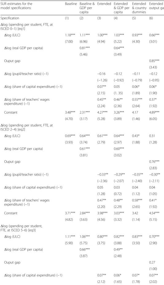
The first thing that needs to be checked is whether the theoretical framework discussed in section 2 is validated by the data. Indeed, for all ‘baseline’and‘extended’ specifica-tions presented in Table 1 below, the coefficient of the unit labour cost, i.e., the wage-productivity differential or simply the‘Baumol’variable, is always significant in all three equations of the system. Moreover, the constant term is also highly significant, espe-cially at primary and secondary levels (for tertiary education the results are more mixed since the constant term is not always statistically significant). This finding confirms the faster rise in education costs relative to the rise in ULCs—a common proxy for captur-ing broad inflationary pressures in (most new-Keynesian) economic models. It also re-veals the most often advocated solution to the ‘cost disease’ problem: since only wage growth in excess of productivity gains would be fed into higher education costs. This suggests productivity growth as a possible long-term remedy (see Wolff et al., 2014).

When comparing the ‘baseline’ with the ‘extended’specification, however, there ap-pears to be a drop in the estimated ‘Baumol’coefficient. The drop seems substantial in the case of pre- and primary (ISCED 0–1) and tertiary education levels (ISCED 5–6), but it must be associated with the introduction of the (lagged) share of teachers’wages as an additional control in the regression.17 This suggests that the share of teachers’ wages is an important determinant—an additional nominal driver of public education costs, though certainly carrying a different content than the ‘Baumol cost’ variable.18 The ‘extended’specification includes the additional controls discussed in section 3.2. For the specifications reported here, I use student/teacher ratios instead of class size due to better data availability. The pupil/teacher ratio (only averages over aggregated ISCED 1–3 levels are available from Eurostat) is highly significant and the estimated coefficients are all negative, pointing at the relevance of this indicator for cost analysis.

Adding real GDP per capita as an additional regressor to either ‘baseline’ or ‘ ex-tended’specifications does not significantly change the estimated coefficients for ULCs. However, it does improve the overall fit of the model (i.e., the R2increases when adding GDP per capita). As evidenced in Table 1, adding GDP per capita seems no more than a better way to control for some remaining country-specific factors (probably not en-tirely removed after first-differentiating the data). Indeed, the specification illustrated in column (5) replaces the GDP per capita with country-specific dummies, which deliver an expected improvement in the overall fit of the model. However, the specification with GDP per capita is preferred by the Akaike (AIC) and Bayesian Information Criter-ion (BIC), with both being larger in the ‘extended & country dummies’compared to

‘extended & GDP per capita’.

Section 2 has provided an extensive discussion on the relevant mechanisms behind the dynamics of education spending; yet, these theoretical mechanisms are assumed to

(11)

Table 1Estimates for public education spending per (FTE) student SUR estimates for the

model specifications:

Baseline Baseline & GDP per capita Extended Extended & GDP per capita Extended & country dummies Extended & output gap Specification (1) (2) (3) (4) (5) (6)

Δlog (spending per student, FTE, at ISCED 0–1) [eq1]

Δlog (ULC) 1.18*** 1.11*** 1.00*** 1.03*** 0.93*** 0.66*** (7.00) (6.96) (4.94) (5.22) (4.30) (3.01)

Δlog (real GDP per capita) 0.81*** 0.64*** (5.46) (3.49)

Ouput gap 0.85***

(3.43)

Δlog (pupil/teacher ratio) (−1) −0.16 −0.12 −0.11 −0.12 (−1.26) (−0.92) (−0.79) (−0.95)

Δlog (share of capital expenditure) (−1) 0.07** 0.05 0.06* 0.06* (2.15) (1. 35) (1.89) (1.90)

Δlog (share of teachers’wages expenditure) (−1)

0.45** 0.46** 0.55*** 0.37* (2.24) (2.36) (2.64) (1.92) Constant 3.48*** 2.31*** 4.27*** 3.26*** 4.17 4.89***

(4.70) (3.17) (5.28) (3.89) (1.46) (6.05)

Δlog (ULC) 0.69*** 0.64*** 0.61*** 0.64*** 0.43* 0.31 (3.93) (3.74) (2.79) (2.97) (1.88) (1.28)

Ouput gap 0.76***

(2.83)

Δlog (pupil/teacher ratio) (−1) −0.33** −0.29** −0.35** −0.30** (−2.36) (−2.07) (−2.40) (−2.11)

Δlog (share of capital expenditure) (−1) 0.05 0.03 0.04 0.04 (1.28) (0.72) (1.12) (1.05)

0.47** 0.48** 0.58*** 0.41* (2.20) (2.29) (2.65) (1.92) Constant 3.71*** 2.84*** 3.98*** 3.03*** 3.42 4.54***

(4.82) (3.63) (4.56) (3.32) (1.14) (5.15)

Δlog (ULC) 1.11*** 1.06*** 0.80*** 0.82*** 0.83*** 0.70*** (5.90) (5.75) (3.75) (3.88) (3.50) (2.90)

Δlog (real GDP per capita) 0.66*** 0.49** (3.87) (2.48)

Ouput gap 0.27

(1.00)

Δlog (share of capital expenditure) (−1) 0.07** 0.06* 0.07* 0.07** (2.12) (1.65) (1.78) (2.02) 0.46** 0.46** 0.55** 0.43**

(12)

work mainly over the long-term. When exploring data with an annual frequency, richer dynamics might be revealed. I rely on the empirical literature to provide some needed guidelines in my investigation. Humphreys (2000) and Delaney and Doyle (2011) among many others find strong evidence that business cycles affect government finan-cial support for higher education. Although primary and secondary education are compulsory and, therefore, should not be too much subject to short-term policy con-siderations, I will include‘output gap’as an additional regressor (i.e., proxy for business cycle) for all levels of education considered. However, I had to remove GDP per capita from this specification (depicted in column (6) in Table 1) to avoid colinearity due to the high correlation between the two indicators; it is interesting to observe that the Baumol coefficient drops significantly or even losses statistical significance in some cases. This finding points to the fact that the output gap and the ULC might both reflect similar information, such as the gap between demand (proxied by the wage component of the ULC) and supply (proxied by the productivity component of the ULC). To select the most parsimonious specification, I rely again on AIC and BIC information criteria. In this case, both parsimony measures (AIC and BIC) prefer the specification that includes GDP per capita (column 4) to the one that includes output gap (column 6).

4.2 A four-equation system

Within the broader context of public budgeting, education spending represents only a minor allocation of public financial resources. According to Eurostat, at the aggregate level of the European Union (EU), education makes up for a little bit more than 10% of total government spending. Over the 2000–2012 period this percentage has varied sig-nificantly across EU member states, from a minimum of 6% in Greece to a maximum of 19% in Estonia. Given this allocation problem, there is a need to account for the existing general public budget constraints when modelling the dynamics of education spending. The Appendix discusses some additional reasons to append a fourth equation to the initial three-equation system.

Table 1Estimates for public education spending per (FTE) student(Continued) Δlog (share of teachers’wages

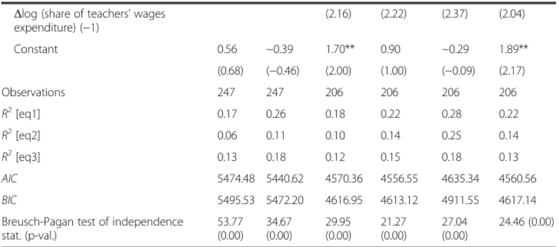
expenditure) (−1) (2.16) (2.22) (2.37) (2.04) Constant 0.56 −0.39 1.70** 0.90 −0.29 1.89** (0.68) (−0.46) (2.00) (1.00) (−0.09) (2.17) Observations 247 247 206 206 206 206 R2[eq1] 0.17 0.26 0.18 0.22 0.28 0.22 R2[eq2] 0.06 0.11 0.10 0.14 0.25 0.14 R2[eq3] 0.13 0.18 0.12 0.15 0.18 0.13 AIC 5474.48 5440.62 4570.36 4556.55 4635.34 4560.56 BIC 5495.53 5472.20 4616.95 4613.12 4911.55 4617.14 Breusch-Pagan test of independence

stat. (p-val.) 53.77 (0.00) 34.67 (0.00) 29.95 (0.00) 21.27 (0.00) 27.04 (0.00) 24.46 (0.00) Note:TheR2

is a summary measure of the overall in-sample predictive power of the model; it is simply computed as 1-residual sum of squares/total sum of squared residuals. The null of the Breusch-Pagan tests is that the residuals across the estimated equations in the model are independent

Country dummies are not shown in specification (5)

(13)

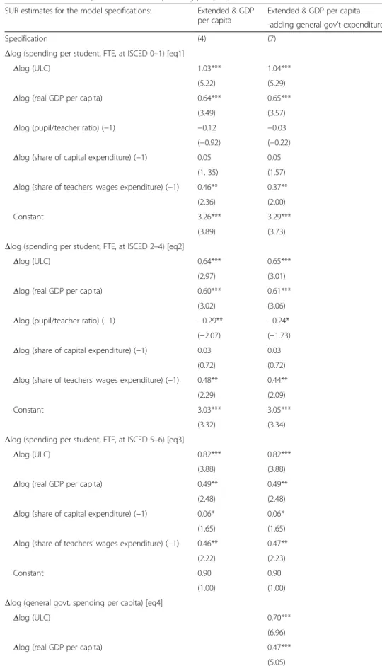
To address this aspect, specification (7) in Table 2 below presents a four-equation system, where the forth equation describes the dynamics of the general public spending

per capita. The initial three-equation system has already addressed the possibility of reallocations (through correlations) between the three relevant education levels: pri-mary, secondary and tertiary. Now, within a four-equation system, the possibility of reallocation between education and other areas of the public budget is also addressed (e.g., spending on economic affairs, military and defense are all substitutes to public education spending, etc.).

The empirical specification of this fourth equation is intentionally kept simple. Baumol’s theory can be easily extended to include all publicly-provided services (same assumptions are needed), while income per capita is one of the most relevant determi-nants for general government spending (see Shelton, 2007). Accordingly, the same two theoretical determinants outlined in the previous sections are included. The coefficients of the first three equations of the system remain basically unchanged between specifica-tions (4) and (7). Interestingly, the fourth equation has a higher explanatory power than the other three, despite relying on just two determinants and a constant term; the constant is statistically significant, though smaller in absolute value than in the case of primary and secondary levels. Other advantages pertaining to specification (7) over specification (4) are highlighted in the Appendix.

Despite all the existing budgetary constraints, some of them arising from the strict EU institutional governance framework, there has always been some degree of domestic policy discretion that could change a given spending allocation due to specific considerations. I intend to reflect the commitment idea using the ‘full’ model specification, which is portrayed by equation (3) from section 3.2. I am making the implicit assumption that policy commitment implies a very clear se-quencing of the decision-making process: current changes in spending allocation to education are decided based on past performances. Compared to the ‘extended’ specification, I now include an additional regressor in each of the three initial equations of the system. In principle, lagged changes in the policy objective (or similar transformations thereof – see below) should represent relevant measures of

past performances. Given the definition of the policy objective,19 a rising share of

early school leavers would reflect a worsening of the situation, while declining ESL shares reflect an improvement (i.e., the lower the ESL shares, the better). Accord-ingly, a truly committed policy-maker would increase spending today (and possibly over the next periods) to counterbalance any unfavourable past developments in the ESL objective. Similarly, a policy-maker could be allowed to reduce spending today if past ESL progress is considered as satisfactory.20

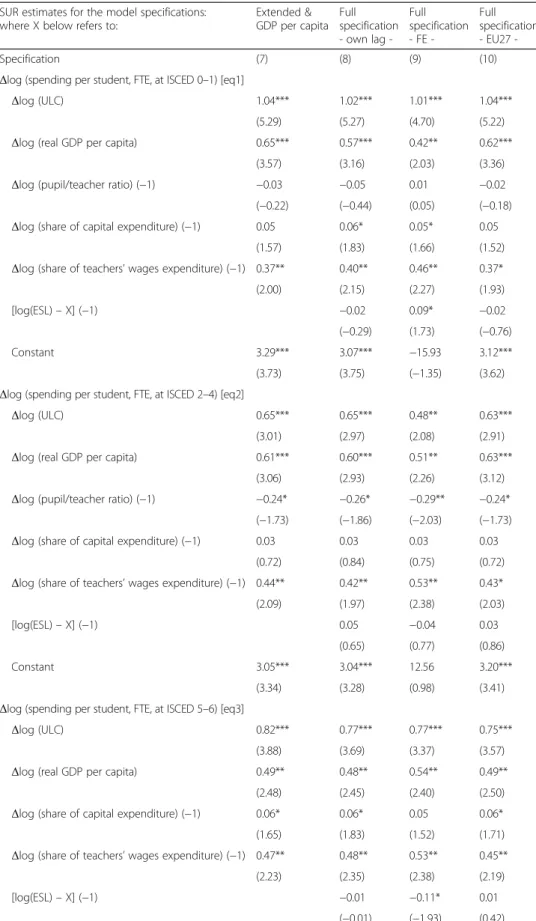
In reality, different EU countries could make different spending allocations despite registering a similar ESL progress; likewise, countries could behave similarly (i.e., increase/decrease education spending by the same percent) despite witnessing very different ESL developments. Given the large diversity in ESL performances21 across the EU members, there is a need to introduce some relevant benchmarks or reference values in order to adequately evaluate/measure the progress registered in the policy object-ive for a gobject-iven country. Despite some inherent simplifications, I present three ways to achieve this goal and illustrate the results in Table 3 below, namely in specifications (8), (9) and (10).

(14)

Table 2Estimates for public education spending per (FTE) student SUR estimates for the model specifications: Extended & GDP

per capita

Extended & GDP per capita -adding general gov’t

expenditure-Specification (4) (7)

Δlog (spending per student, FTE, at ISCED 0_–1) [eq1]

Δlog (ULC) 1.03*** 1.04***

(5.22) (5.29)

Δlog (pupil/teacher ratio) (₋1) ₋0.12 ₋0.03 (₋0.92) (₋0.22)

Δlog (share of capital expenditure) (₋1) 0.05 0.05 (1. 35) (1.57)

Δlog (share of teachers’wages expenditure) (−1) 0.46** 0.37** (2.36) (2.00)

Constant 3.26*** 3.29***

(3.89) (3.73)

Δlog (ULC) 0.64*** 0.65***

(2.97) (3.01)

Δlog (pupil/teacher ratio) (₋1) ₋0.29** ₋0.24* (₋2.07) (₋1.73)

Δlog (share of capital expenditure) (₋1) 0.03 0.03 (0.72) (0.72)

Δlog (share of teachers_’wages expenditure) (₋1) 0.48** 0.44** (2.29) (2.09)

Constant 3.03*** 3.05***

(3.32) (3.34)

Δlog (ULC) 0.82*** 0.82***

(3.88) (3.88)

Δlog (real GDP per capita) 0.49** 0.49** (2.48) (2.48)

Δlog (share of capital expenditure) (−1) 0.06* 0.06* (1.65) (1.65)

Δlog (share of teachers_’wages expenditure) (₋1) 0.46** 0.47** (2.22) (2.23)

Constant 0.90 0.90

(1.00) (1.00)

Δlog (general govt. spending per capita) [eq4]

Δlog (ULC) 0.70***

(6.96)

Δlog (real GDP per capita) 0.47***

(15)

Firstly, I use the laggedchangein ESL as the easiest way to include a feedback mechanism into my specification, which states the policy decision rule dictating howcurrentspending is adjusted. This specification corresponds to column (8) in Table3below and is labelled as‘own lag’because progress in the ESL objective is measured against itsown lag. The intuition is that a policy-maker would compare the available(t-1)ESL value with its previous,(t-2), ESL value to quantify progress before deciding on education spending for the current time period,t. Consequently, the additional regressor included in specification (8) is given by:Δlog(ESL)t-1or,

equivalently, by the difference defined in ESL levels: log(ESL)t-1–log(ESL)t-2.

Secondly, for specification (9) in Table3, I consider that the policy-maker evaluates the available (t-1) ESL value against a fixed (time-invariant) unobserved country-specific reference value. Such a reference value could be either a fixed target or an optimal determined ESL value, though here I include dummy variables to balance the lack of such country-specific measures over the whole estimation period.22This specification, which I label as‘FE’, also controls for any remaining cross-sectional heterogeneity not accounted for so far by the‘full’model specification. Consequently, I include log(ESL)t-1as an additional regressor along with a country-specific dummy.

Thirdly, I consider that, for a given country, the relevant reference value to measure the progress registered by its ESL objective is the EU-aggregate ESL value. This specification, labelled as‘EU27’, corresponds to column (10) in Table3. Consequently, the regressor included in the model is given by the difference between the country-specific ESL and the EU2723average ESL, i.e., log(ESL)t-1–log(ESLEU27)t-1.

In practice, it is more likely that policy-makers rely on a series of benchmarks and reference values (possibly including the ones employed above, i.e., own lags, specific targets, EU averages etc.) to evaluate their progress and decide spending allocations in education. Based on the results displayed in Table 3, there is some weak statis-tical evidence of policy commitment in specification (9), where dummies were in-troduced as a proxy for fixed ESL targets. This evidence should be understood within the limits of the approach considered here. Interestingly, in model (9) the

Table 2Estimates for public education spending per (FTE) student(Continued)

Constant 2.31*** (5.36) Observations 206 206 R2_[eq1] _0.22 _0.22 R2_[eq2] _0.14 _0.14 R2_[eq3] _0.15 _0.15 R2_[eq4] _0.27 AIC 4556.55 5774.34 BIC 4613.12 5840.90

Breusch-Pagan test of independence stat. (p-val.) 21.27 (0.00) 38.23 (0.00)

Note:TheR2

is just a summary measure of the overall in-sample predictive power of the model; it is simply computed as 1-residual sum of squares/total sum of squared residuals. The null of the Breusch-Pagan tests is that the residuals across the estimated equations in the model are independent

(16)

Table 3Estimates for public education spending per (FTE) student with policy commitment SUR estimates for the model specifications:

where X below refers to:

Extended & GDP per capita Full specification own lag -Full specification FE -Full specification EU27 -Specification (7) (8) (9) (10)

Δlog (ULC) 1.04*** 1.02*** 1.01*** 1.04***

(5.29) (5.27) (4.70) (5.22)

Δlog (real GDP per capita) 0.65*** 0.57*** 0.42** 0.62*** (3.57) (3.16) (2.03) (3.36)

Δlog (pupil/teacher ratio) (−1) −0.03 −0.05 0.01 −0.02 (−0.22) (−0.44) (0.05) (−0.18)

Δlog (share of capital expenditure) (−1) 0.05 0.06* 0.05* 0.05 (1.57) (1.83) (1.66) (1.52)

Δlog (share of teachers’wages expenditure) (−1) 0.37** 0.40** 0.46** 0.37* (2.00) (2.15) (2.27) (1.93)

[log(ESL)–X] (−1) −0.02 0.09* −0.02

(−0.29) (1.73) (−0.76)

Constant 3.29*** 3.07*** −15.93 3.12***

(3.73) (3.75) (−1.35) (3.62)

Δlog (ULC) 0.65*** 0.65*** 0.48** 0.63***

(3.01) (2.97) (2.08) (2.91)

Δlog (real GDP per capita) 0.61*** 0.60*** 0.51** 0.63*** (3.06) (2.93) (2.26) (3.12)

Δlog (pupil/teacher ratio) (−1) −0.24* −0.26* −0.29** −0.24* (−1.73) (−1.86) (−2.03) (−1.73)

Δlog (share of teachers’wages expenditure) (−1) 0.44** 0.42** 0.53** 0.43* (2.09) (1.97) (2.38) (2.03)

[log(ESL)–X] (−1) 0.05 −0.04 0.03

(0.65) (0.77) (0.86)

Constant 3.05*** 3.04*** 12.56 3.20***

(3.34) (3.28) (0.98) (3.41)

Δlog (ULC) 0.82*** 0.77*** 0.77*** 0.75***

(3.88) (3.69) (3.37) (3.57)

Δlog (real GDP per capita) 0.49** 0.48** 0.54** 0.49** (2.48) (2.45) (2.40) (2.50)

Δlog (share of capital expenditure) (−1) 0.06* 0.06* 0.05 0.06* (1.65) (1.83) (1.52) (1.71)

Δlog (share of teachers’wages expenditure) (−1) 0.47** 0.48** 0.53** 0.45** (2.23) (2.35) (2.38) (2.19)

[log(ESL)–X] (−1) −0.01 −0.11* 0.01

(17)

coefficient associated with the commitment proxy is positive for primary education but negative for tertiary education, meaning that, for example, if previous ESL values were above a fixed (country-specific) reference value, spending would in-crease at the primary (including pre-primary) but dein-crease at the tertiary education level – a result that makes sense given that the policy objective is expressed in terms of school dropouts with less than (upper) secondary education. Unfortu-nately, such weak statistical evidence does not allow me to draw strong conclusions with respect to policy commitment in this empirical setting. The explanation could be related to large data heterogeneity issues, most likely due to the presence of some gross outliers in the sample (see Appendix) or simply because the model tries to pool together countries with very different policy attitudes. Empirical re-sults were sensitive to sample length changes, i.e., dropping more than one obser-vation either from the beginning or from the end of the sample would alter the coefficients and their statistical significance; a future investigation that could lever-age on better data availability and span over longer time periods should perhaps come with more insights and more robust findings. Probably more interesting, the results were not that sensitive when dropping some of the selected controls that define the ‘extended’specification.

4.3 Policy discussion

With public education costs growing faster than aggregate prices, affordability concerns inevitably arise in any discussion on public education investment. The empirical results

Table 3Estimates for public education spending per (FTE) student with policy commitment (Continued)

Constant 0.90 0.96 23.31 0.97

(1.00) (1.09) (1.81) (1.07)

Δlog (general spending per capita) [eq4]

Δlog (ULC) 0.70*** 0.69*** 0.69*** 0.69***

(6.96) (6.83) (6.86) (6.86)

Δlog (real GDP per capita) 0.47*** 0.46*** 0.46*** 0.46*** (5.05) (4.85) (4.95) (4.95) Constant 2.31*** 2.25*** 2.27*** 2.27*** (5.36) (5.21) (5.27) (5.27) Observations 206 200 203 203 R2[eq1] 0.22 0.23 0.31 0.22 R2[eq2] 0.14 0.14 0.26 0.14 R2[eq3] 0.15 0.15 0.23 0.14 R2[eq4] 0.27 0.26 0.26 0.26 AIC 5774.34 5591.05 5755.20 5693.97 BIC 5840.90 5666.91 6060.01 5770.17

Country dummies No No Yes No

Breusch-Pagan test of independence stat. (p-val.) 38.23 (0.00) 32.98 (0.00) 36.23 (0.00) 37.70 (0.00)

Note:The R2

is just a summary measure of the overall in-sample predictive power of the model; it is simply computed as 1-residual sum of squares/total sum of squared residuals. The null of the Breusch-Pagan tests is that the residuals across the estimated equations in the model are independent

Country dummies not shown for specification (9)

(18)

above have exposed the ‘cost disease’as a common phenomenon across the EU, espe-cially at primary and secondary education levels. In the case of higher education in-stead, the results were more mixed (see Table 1), probably due to the nature of the data employed in the empirical analysis, which covers only public funding sources but disre-gards spending by households, philanthropists, international institutions, etc. In contrast to primary and secondary education, public financial support for tertiary edu-cation (which is generally not mandatory) covers only a part of total eduedu-cation costs (with the remaining being filled from private sources). In this context, such mixed re-sults for tertiary education are not quite unexpected. In fact, some recent policy initia-tives envisaging a shift in the cost burden from governments to parents and/or students have been taken mainly with respect to tertiary education funding support (e.g., via higher tuition fees, fiscal incentives for student loans, etc.). If this trend in pol-icy changes will continue in the future, it would definitely help to reduce pressure on public budgets. Some forms of cost-sharing might also arise at lower education levels like, for example, private tutoring to compensate for poor/insufficient teaching that usually arises as a consequence of lower public financial support. However, there are good reasons to expect harder public scrutiny in case these practices become the norm rather than the exception (the last paragraph in section 2 lists some reference studies discussing the interaction between education and redistribution policies, and the preferences of the median-voter).

As already suggested in section 4.1 above, growing labour productivity (at least at a faster pace than wages so that unit labour costs are kept in check) might be a way to tackle the‘cost disease’problem over the long-term. Indeed, the‘progressive’sector can more efficiently leverage physical capital and technology to deliver overall productivity gains (despite stagnation in other sectors). However, this productivity-enhancing mech-anism can be strengthened when human capital (instead of simply labour) enters the production function of the ‘progressive’sector. In fact, some recent extensions of the Baumol model include more positive interactions between the ‘progressive’ and the

‘stagnant’sectors as a way to achieve better economic outcomes (see Pugno, 2006). The dual causality link between education and economic development exposes, neverthe-less, a range of effective policy options in this context. More importantly, it highlights a mechanism along which better designed policies can incentivize more (or more effi-cient) human capital accumulation, not only through the consumption of education services, but also through other forms, such as learning-by-doing, up-skilling, lifelong learning, etc.

It is important to note that some forms of human capital investment do not necessar-ily require public financial support (e.g., learning-by-doing), but others do so, and sometimes to a large extent (besides education, other examples include re-training and some active labour market policies). From a political economy perspective, and apart from business cycle influences, it is clear that policy-makers can shift their preferences between (short-term) redistributive policies (e.g., transfers or subsidies) and policies in-centivizing (long-term) human capital accumulation. There are probably many difficult trade-offs here that arise due to seemingly conflicting objectives. Yet, it is not necessar-ily the size of public spending allocated to a given policy area that this paper is con-cerned with, but rather the policy-decision process of adjusting/amending spending in an effort to deliver results on a clear policy mandate. In this context, the weakoverall

(19)

empirical evidence found for policy commitment on education could highlight risks as-sociated with EU economic development prospects. Even if the lack of clear evidence for commitment is mostly a reflection of large heterogeneity issues in the data, it could nevertheless raise concerns with respect to real (economic and political) convergence prospectsin Europe.

5 Conclusions

This paper makes two important contributions. Firstly, it uncovers some of the main economic determinants driving the dynamics of public education spending in a panel dataset spanning across EU members over the 2000–2012 period. The empirical model builds mainly on theoretical insights borrowed from Baumol (1967), Baumol and Bowen (1966), and Bowen (1980). A four-equation system is proposed to resolve the spending allocation problem inherent in a public budgeting process, with three equa-tions describing the dynamics of education spending per student (at primary, secondary and tertiary levels) and a fourth one describing the dynamics of total public spending in per capita terms. The empirical results provide strong evidence that the costs of pub-lic education have been rising faster than general prices (proxied here by the aggregate unit labour costs), despite accounting for growing real income/demand effects (proxied by GDP per capita). Besides confirming the theories on which the specification of the model was built, such a finding also exposes, unfortunately, the long-term affordability challenge of public education investment.

Secondly, the empirical setting above is used to investigate whether policy commit-ment has been a major determinant driving the dynamics of public education spending in Europe. I draw on two main policy agendas and select the share of early school leavers as a relevant policy objective for the EU member states over the whole 2000–2012 period. Then, expanding on the previous model specification, I formulate an empirical equivalent of a policy rule that would determine how education spending decisions are related to past progresses in the policy objective. Nonetheless, I find only weak overall statistical evidence of policy commitment to education across Europe, most likely due to large heterogeneity issues in the dataset. Moreover, the empirical results seem to be sensitive to some basic robustness checks.

Finally, it might be worth pointing out some further research directions. A possible follow-up could attempt to include determinants that draw more heavily on political economy considerations to reflect changes in political and/or institutional aspects, different financing mechanisms, or analyse longer time periods (see Busemeyer, 2007). Moreover, direct extensions of the present analysis of commitment to other policy domains remain possible, especially in the area of employment and social security, although a different theoretical background would be required in this case.

Endnotes

1

See the official communication of the European Council from March 2000 at http:// www.consilium.europa.eu/en/uedocs/cms_data/docs/pressdata/en/ec/00100-r1.en0.htm and the conclusions of the European Council from June 2010 at http://www.consilium. europa.eu/ueDocs/cms_Data/docs/pressData/en/ec/115346.pdf.

2

As an additional proof of its policy relevance, an ambitious EU-wide target of no more than 10 % was initially specified, and later reiterated within the Europe 2020

(20)

version together with country-specific targets, in an attempt to enforce more efficient implementation and accountability.

3

How much a government spends on education can be seen as a measure of its com-mitment to education according to Gylfason (2001). Some existing theoretical studies address the issue of policy commitment and time-consistent fiscal policy in general, but with careful considerations with respect to education investment in particular, e.g., Boadway et al. (1996), Gradstein (2000), Andersson and Konrad (2003).

4

An interesting analysis in the EU context is provided in Dragomirescu-Gaina et al. (2015), who discuss the positive interactions between labour productivity and education choices with a long-term perspective.

5

Same arguments can be made if one groups public spending on education and health-care together (as long-term investments in human capital) and contrasts them with spending on other public policy areas like employment and social security (which can also be seen as investments in human capital, but from a rather short-term perspective).

6

This can be seen mostly in the significant drop in the relative prices of information-communication & technology (ICT) equipment (compared to general prices) over the last decades.

7

Besides labour mobility, several other factors might also contribute: nominal rigidi-ties in setting wages, high unionization levels etc.

8

At this point, an interested reader might notice the striking similarities between the work of Baumol and the parallel research in international economics done by Balassa (1964) and Samuelson (1964). In a similar modelling setting, two sectors (i.e., the trad-able and the non-tradtrad-able sector) are characterized by different productivity dynamics, but the convergence of nominal wages later drives domestic inflation higher and gener-ates real appreciation of the domestic currency.

9

This paper uses first-differences of the data, but a very similar approach is employed in Busemeyer (2007), who uses the residuals from an estimated autoregressive AR(1) model in levels.

10

See Jefferson (2005) for a survey on empirical evidence related to the causality link between education financing and students’performances. Two more recent but exten-sive reviews of the previous literature that are on school and teacher’s characteristics are Hanushek and Woessmann (2010) and Glewwe et al. (2011).

11

For example Gundlach et al. (2001) compute sector-specific productivity in the education sector based on the results of standardized achievement tests for U.S.

12

Heterogeneity might still remain an unsolved issue, despite estimating a model specification in first-differences that control for time invariant characteristics.

13

The inclusion in the regression of the capital expenditures’share instead of non-personnel costs’share (which is the second biggest contributor to total public education spending) is just a matter of choice. Obviously, one cannot include all three compo-nents of public education spending due to collinearity concerns. In this case, capital spending might even provide a clearer interpretation of the results because of its expli-cit content.

14

One can argue (and this would be in line with some existing empirical studies) that teachers’age and gender composition are also important determinants of overall educa-tion spending; yet, data availability was the main drawback for not using more detailed

(21)

indicators as controls. Also, one should be careful not to overstate the importance of some qualitativeindicators in a time-series analysis; most of these indicators, e.g., de-scribing schools’organizational methods or other institutional dimensions, might have only a one-time effect (see discussion in Wolff et al., 2014) and would therefore not appear as significant in a time-series regression analysis.

15

Please note that this would not represent an empirical formulation of a transmission mechanism—from spending public resources to reaching specific outcomes—mainly because the causality in the text above runs backwards.

16

The number of FTE pupil/students used to compute the COFOG-based spending per student at the ISCED 0–1 level correspond only to ISCED 1 pupils, thus excluding ISCED 0 pupils.

17

This is a common finding in empirical studies when the two regressors involved are correlated. However, in my case, the correlation is not high enough to render any of the coefficients statistically insignificant. Therefore, I take this as evidence of their different content and significance in explaining the dynamics of education spending.

18

In principle, the share of teachers’ wages in education spending would reflect the sensitive balance that governments need to strike between human (e.g., teachers) and physical capital (e.g., schools) when it comes to allocating public funds.

19

Although not explicitly treated here, educationqualitymight be an important elem-ent in the policy discussion. Still, it remains an open question whether consistelem-ent (as opposed to one-time) improvements in education quality are possible at all (see Wolff et al., 2014). Meanwhile, there is plenty of space to improve the existing quantitative

measures of education attainment, such as ESL.

20

A never-ending quest for lower ESL values would be inefficient and waste import-ant financial resources when policy-makers face an allocation problem and different policy objectives. Moreover, given the increased efforts to foster mobility across EU countries (e.g., ERASMUS+), most differences between countries should be mitigated through migration or internationalization of education over the long-run. In light of these arguments,‘policy commitment’appears also in the reverse situation when spend-ing is reduced if the progress is satisfactory, thus facilitatspend-ing a linear interpretation of the model.

21

Historically, some EU countries have consistently registered very low ESL values over the 2000–2012 period, among them: AT, CZ, DK, FI, HR, LT, PL, SE, SI and SK. Other members such as CY, DE, FR, IE, LU and NL have managed to reach single-digit ESL levels only over the most recent years (i.e., 2010–2012). The rest of the EU mem-bers (representing about half of the total EU28) were still above the 10 % EU-wide tar-get as of 2012.

22

Europe 2020 agenda has introduced country-specific targets for ESL. However, these targets were adopted after the year 2010 (though at different moments) and were therefore not available for most of the period under consideration here. Only as an exercise, I have used the deviations from these politically ‘announced’country-specific targets, but the results were not significant (result are available from the author). If anything, this highlights the lack of relevance (both political and empirical) of the an-nounced targets, thus supporting the use of a series of reference values in the present evaluation of policy commitment.

23

(22)

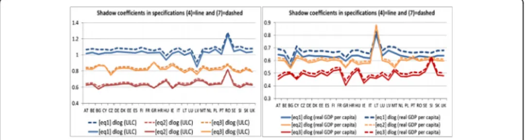
Appendix

This appendix presents a sensitivity check of the estimated model coefficients displayed for both specifications (4) and (7) in Table 2. This sensitivity check addresses hetero-geneity concerns with respect to countries included in the sample and consists in esti-mating the same model specification, but excluding one country at a time. The resulting ‘shadow coefficients’are plotted in the figure below, where the x-axis lists the excluded country. The advantages of a four-equation system can be most clearly ex-posed using a simple standard deviation measure to reflect the departure of the‘shadow coefficients’from the ones reported in specifications (4) or (7). What is probably less clear in the figure, but becomes evident when displaying the raw standard deviations (henceforth sdev.) of the ‘shadow coefficients’, is that the outliers now play a less important role (though the bias in the estimated coefficients cannot be entirely elimi-nated). The three-equation system exhibits a sdev. of 5.94, 4.29 and 3.44% for the

‘shadow coefficients associated with ULCs in equations 1, 2, and 3, respectively, and 4.02, 5.82 and 3.75% for GDP per capita. Similarly, the four-equation system exhibits a sdev. of 5.46, 4.19 and 3.12% for ULCs in equations 1, 2, and 3, respectively, and 3.73, 5.77 and 3.59% for GDP per capita.

Moreover, the figure above suggests that the overall sample might contain some gross outliers (which seem to introduce a bias in the estimated coefficients) such as: BG, CY, CZ, GR, HU, LT, LV, MT, RO, and SI. These findings are not surprising since some of these countries have suffered harsh adjustments in their fiscal policies, including their public expenditures: RO, LT and LV implemented broad austerity programs negotiated with the international financial institutions, mostly in 2010 (the 25% cut in public wages in RO and LV, and the 15% cut in LT have mostly affected education, health-care and other related public sectors with large employment shares). Others such as GR, and to a smaller extent HU, have been among the countries that required international financial assistance in the aftermath of the recent global economic and European sover-eign crisis. Countries such as ES, IE, IT, and PT have also benefited from different forms of EU financial support, but these countries do not seem to bias the estimated

‘shadow coefficients’ according to the figure above. However, most (if not all) EU members have undertaken some adjustments in their public spending policies over the recent periods, especially as a consequence of the sovereign crisis that has increased the pressure on public finances across the board.

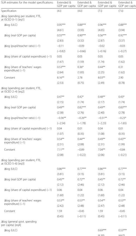
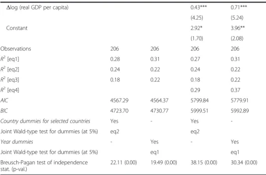
Just as an illustration of the possible effects introduced in the model by the outliers identified above and/or the recent European sovereign crisis, I depart from

(23)

Table 4Alternative estimates for public education spending per (FTE) student–tackling outliers SUR estimates for the model specifications: Extended &

GDP per capita Extended & GDP per capita Extended & GDP per capita Extended & GDP per capita

Specification (4.i) (4.ii) (7.i) (7.ii)

Δlog (ULC) 0.95*** 0.88*** 0.96*** 0.88***

(4.61) (3.93) (4.65) (3.94)

Δlog (real GDP per capita) 0.55*** 0.90*** 0.56*** 0.92*** (2.83) (3.32) (2.87) (3.37)

Δlog (pupil/teacher ratio) (−1) −0.11 −0.09 −0.02 −0.03 (−0.82) (−0.66) (−0.16) (−0.27)

0.53*** 0.36* 0.44** 0.31 (2.64) (1.83) (2.25) (1.62)

Constant 8.16** 2.78 8.03** 2.90

(2.53) (0.75) (2.49) (0.78)

Δlog (ULC) 0.47** 0.42* 0.48** 0.43*

(2.15) (1.74) (2.17) (1.74)

Δlog (real GDP per capita) 0.49** 0.82*** 0.49** 0.83*** (2.38) (2.76) (2.40) (2.78)

Δlog (pupil/teacher ratio) (−1) −0.36** −0.26** −0.31** −0.23* (−2.54) (−1.78) (−2.23) (−1.65)

0.54** 0.44** 0.49** 0.43** (2.51) (2.08) (2.31) (1.99)

Constant 7.11** −0.89 7.04** −0.84

(2.08) (−0.22) (2.06) (−0.21)

Δlog (ULC) 0.86*** 0.77*** 0.86*** 0.77***

(3.81) (3.15) (3.81) (3.15)

Δlog (real GDP per capita) 0.45** 0.72** 0.45** 0.72** (2.12) (2.46) (2.12) (2.46)

0.53** 0.53** 0.54** 0.53** (2.42) (2.48) (2.47) (2.48)

Constant 1.59 −0.45 1.59 −0.45

(0.45) (−0.11) (0.45) (−0.11)

Δlog (general govt. spending per capita) [eq4]

Δlog (ULC) 0.69*** 0.53***