Aggregate hiring and the value of jobs along the business cycle

Aggregate Hiring and the Value of Jobs Along the

Business Cycle

Eran Yashiv

Tel Aviv University, CfM (London School of Economics), and CEPR November 14, 2016

Abstract

U.S. CPS data indicate that in recessions firms actuallyincreasetheir hiring rates from the pools of the unemployed and out of the labor force. Why so? The paper provides an explanation by studying the optimal recruiting behavior of the rep-resentative firm. The model combines labor frictions, of the search and matching type, with capital frictions, of the q-model type.

Optimal firm behavior is a function of the value of jobs, i.e., the expected present value of the marginal worker to the firm. These are estimated to be counter-cyclical, the underlying reason being the dynamic behavior of the labor share of GDP. The counter-cyclicality of hiring rates and job values, which may appear counter-intuitive, is shown to be consistent with well-known business cycle facts. The analysis em-phasizes the difference between current labor productivity and the wider, forward-looking concept of job values.

The paper explains the high volatility of firm recruiting behavior, as well as the reduction over time in labor market fluidity in the U.S., using the same estimated model. Part of the explanation has to do with job values and another part with the interaction of hiring and investment costs, both determinants having been typically overlooked.

Key words:counter-cyclical job values, business cycles, aggregate hiring, , vacan-cies, labor market frictions, capital market frictions, volatility, labor market fluidity.

Aggregate Hiring and the Value of Jobs Along the Business Cycle1

1

Introduction

The paper asks what governs the representative firm hiring behavior along the busi-ness cycle. This behavior is important for our understanding of busibusi-ness cycles and employment dynamics. The literature on this topic has devoted an enormous amount of attention, for over a decade, to the ability of models to account for the high volatility of job vacancies and unemployment, and has paid much less attention to the counter-cyclicality of the hiring rate from non-employment observed in U.S. data. This paper shows that a model combining labor frictions, of the search and matching type, with capital frictions, of the q-model type, can account for both the high volatility of job vacancy rates and the counter-cyclicality of hiring rates from non-employment. The results of estimation are shown to be consistent with well-known business cycle facts, such as pro-cyclical employment and pro-cyclical vacancy and job-finding rates, as well as job to job flows. The analysis emphasizes the difference between the behavior of cur-rent labor productivity and the wider, forward-looking concept of job value.

I look at the optimality equation of the firm, which equates the marginal cost of worker recruitment and the expected present value of the worker for the firm, i.e., the job value. I estimate alternative specifications of the equation. Estimation rests on key formulations in the literature, particularly the ones related to search and matching and investment q models. Following estimation, I analyze the cyclical behavior and volatility of job values and of the recruiting variables.

The main findings are as follows:

(i) Job values are counter-cyclical in U.S. data. This key finding means that in

re-cessions the value of jobs for firms goesup. Note that this value is a forward-looking

expected present value of future labor profitability.

(ii) Correspondingly, hiring rates from non-employment (unemployment + out of the labor force) are counter-cyclical: it is worthwhile for firms to increase hiring rates as job values rise in recessions.

(iii) While the afore-mentioned hiring rates are counter-cyclical, vacancy rates and hiring rates from employment (i.e., job to job flows) are pro-cyclical. The differences

1_{I am grateful to Larry Christiano and Giuseppe Moscarini for very useful discussions; to seminar partcipants at} the Dale Mortensen memorial conference (Aarhus, October 2014) and at the CEPR ESSIM conference (Tarragona, May 2015) for useful feedback; and to Avihai Lifschitz, Andrey Perlin and Ziv Usha for excellent research assistance. Any errors are my own.

between points (ii) and (iii) are explained.

(iv) While point (i), the counter-cyclicality of job values, may appear counter-intuitive, it is consistent with the findings of recent studies looking at the cyclical behavior of the labor share in GDP. It is the dynamic behavior of the labor share that engenders the counter-cyclicality of the forward-looking job values.

(v) Points (i) and (ii) do not contradict what we already know about the cyclical features of the labor market, including pro-cyclical employment job finding rates, and wages.

(vi) Moving from cyclicality to volatility, the high volatility of vacancy and hiring rates is explained within the same framework. Part of the explanation has to do with job values and another part with the interaction of recruitment behavior with capital investment behavior. Both determinants have been typically overlooked.

(vii) The secular phenomenon of a reduction in labor market fluidity in the U.S. over time, noted by Davis and Haltiwanger (2014), is also accounted for, using the same framework.

The paper proceeds as follows: Section 2 presents the context of the paper in the lit-erature. Section 3 presents the model and the key relations to be examined empirically. Section 4 studies the cyclical behavior of the key data series. The data and methodol-ogy are elaborated in Section 5, followed by the results of estimation in Section 6. The cyclical implications of the results are elaborated in Section 7. Section 8 elaborates on the connections of the results to the cyclicality of the labor share in GDP, recently dis-cussed in other Macro contexts. Section 9 studies the volatility of the recruitment series (vacancy and hiring rates) and relates them to the estimated job values. In Section 10 I use this framework to explain the decline in U.S. labor market fluidity. Section 11 concludes. Derivations and other technical matters are relegated to appendices.

2

The Paper in the Context of the Literature

This paper focuses on the firms’ optimal recruiting behavior in the presence of frictions in an aggregate context along the business cycle. To see how recent literature has ap-proached this topic, it may be useful to discuss this behavior using the following simple equation:

MCt( ) =EtPVt( ) (1)

with the marginal benefit, which is the expected present value of what the firm will get from the employment relationship. In search and matching models this is usually the free entry condition. Table 1 lists 13 key studies and reports what these studies have posited with respect to the LHS and the RHS of equation (1). Appendix A presents the full equation as formulated by each study. The studies are divided into two groups – those positing linear costs and those positing convex costs.

Table 1

Beyond the differences between linear and convex costs, the table shows that the different permutations of formulating the equation include:

(i) Single job vs large firms.

(ii) Using vacancies or actual hires as arguments of the cost function.

(iii) Formulating labor only or capital and labor as determining productivity. (iv) Wages (appearing on the RHS) being determined by the Nash solution, in-trafirm bargaining, credible bargaining or sticky wage mechanisms.

(v) Worker separations modeled as exogenous or endogenous, constant or stochas-tic.

(vi) Discounting the future with a constant or time-varying rate; for the latter, there are different formulations (IMRS, WACC or derived from the stock market).

The current paper looks at a number of alternative specifications. The key one has large firms and convex costs; takes into account both vacancies and actual hires as ar-guments of the cost function; includes capital as well as labor; models capital adjust-ment frictions as well as labor frictions; uses actual wages and separation rates, without explicitly modelling how they are determined; and uses a time-varying IMRS-type dis-count rate. The idea is to structurally estimate this equation (and any accompanying one) in order to explore the cyclicality and volatility of aggregate recruitment behavior. In previous work – Merz and Yashiv (2007) and Yashiv (2016) – I have also used this formulation, or special cases of it.

The former paper did so in the context of studying the determinants of the market value of U.S. firms. The idea there is that the value of investment and the value of hiring make up the value of the firm. That paper thus focuses on matching stock market values and uses relevant financial data in estimation. The current paper does not deal at all with stock market issues and does not use financial data.

The latter paper uses the formulation above to analyze the joint, forward-looking behavior of hiring and investment. It looks at their inter-relationships and the deter-minants of their inter-connected present values. It takes a Finance-like approach in

treating job values and capital values akin to stock prices. The empirical work is a VAR forecast analysis which allows for the determination of the relative importance of various variables in accounting for these “stock prices.” Hence it decomposes job and capital values into “dividend” and “discounting” components, as the Finance literature does.

The current paper focuses on job values only and the key issue is firm recruiting behavior over the business cycle. In particular, the current paper (i) explores the cycli-cal behavior of the key series related to recruiting; (ii) relates job value behavior to the labor share over the cycle; (iii) explores the relationship between the different recruit-ing series – vacancy rates and two hirrecruit-ing rate series – and job values along the cycle; (iv) shows that the standard search and matching model is not able to account for the cyclical patterns; (v) shows how the current model explains the high volatility of the recruitment rates; (vi) studies the secular decline in labor market fluidity, including recruiting.

Thus, the reader learns different lessons: Merz and Yashiv (2007) show that stock prices/values of firms depend on capital and job values and quantify these relations. Yashiv (2016) shows the complementarity between the hiring and investment processes; the important cross effects of the value of capital on the mean and the volatility of the hiring rate, and vice versa; and that future returns play a dominant role in determining capital and job values. The current paper shows that hiring rates from non-employment are counter-cyclical, following the counter-cyclicality of job values; it shows that the underlying reason is the dynamic behavior of the labor share of GDP; and that while this counter-cyclicality may appear counter-intuitive, it is consistent with well-known business cycle facts; and it shows that the same model can account for high volatility and the secular decline of the recruiting variables.

3

The Model

I present a model of firm optimization, which includes capital as well as labor, and formulate the costs function underlying the problem in such a way that the cases shown in Table 1 above will mostly be special cases.

3.1 The General Model

Set-Up. There are identical workers and identical firms, who live forever and have

Worker Flows. Consider worker flows. The flow from non-employment –

unemploy-ment (U) and out of the labor force (O) – to employunemploy-ment,E, is to be denotedOE+UE

and the separation flow in the opposite direction, EU+EO. Worker flows within

em-ployment – i.e., job to job flows – are to be denotedEE.

I shall denote: h n = h1 n + h2 n (2) h1 n = OE+UE E ; h2 n = EE E

Henceh1_andh2 _{denote flows from non-employment and from other employment,}

respectively, andnis employment.

Separation rates are given in an analogous way by:

ψ = ψ1+ψ2 (3) ψ1 = EO+EU E ; ψ 2₌ EE E = h2 n Employment dynamics are thus given by:

nt+1 = (1 ψ1_t ψ2_t)nt+h1t +h2t (4)

= (1 ψ_t)nt+ht, 0 ψ_t 1 h2_t = ψ2_tnt

Matching and Separations.2 Firms hire from non-employment (h1_t) and from other

firms (h2_t). Each period, the worker’s effective units of labor (normally 1 per person)

depreciate to 0, in the current firm, with some exogenous probability ψ_t. Thus, the

match suffers an irreversible idiosyncratic shock that makes it no longer viable. The worker may be reallocated to a new firm where his/her productivity is (temporarily)

restored to 1. This happens with a probability of ψ2_t. Those who are not reallocated

join unemployment, with probability ψ1_t = ψ_t ψ2_t. So the fractionψ2_t that enters job

to job flows depends on the endogenous hiring flow h2_t. The firm decides how many

vacancies vt to open and, given job filling rates (q1t,q2t), will get to hire from the

existing non-employed and from the pool of matches just gone sour. The job-filling or matching rates satisfy:

q1_t = h 1 t vt ; q2_t = h 2 t vt ; qt =q1t +q2t

Firms Optimization. Firms make gross investment (it)and vacancy (vt)decisions.

Once a new worker is hired, the firm pays him or her a per-period wage wt. Firms

use physical capital (kt) and labor (nt) as inputs in order to produce output goods yt

according to a constant-returns-to-scale production function f with productivity shock

zt:

yt = f(zt,nt,kt), (5)

Gross hiring and gross investment are subject to frictions, spelled out below, and

hence are costly activities. I represent these costs by a function g[it,kt,vt,ht,nt]which

is convex in the firm’s decision variables (it,vt,) and exhibits constant returns-to-scale,

allowing hiring costs and investment costs to interact.

In every period t, the capital stock depreciates at the rate δt and is augmented by

new investmentit. Similarly, workers separate at the rateψ_tand the employment stock

is augmented by new hiresqtvt =ht. The laws of motion are:

kt+1 = (1 δt)kt+it, 0 δt 1. (6)

nt+1= (1 ψ_t)nt+qtvt, 0 ψ_t 1 (7)

The representative firm chooses sequences ofitandvtin order to maximize its

prof-its as follows: max fit+j,vt+jg Et ∞

∑

∏

subject to the constraints (6) and (7), where τt is the corporate income tax rate, wt is

the wage,χ_t the investment tax credit, Dt the present discounted value of capital

de-preciation allowances, ˜pI_t the real pre-tax price of investment goods, andρ_t+j is a

time-varying discount factor. The firm takes the paths of the variablesqt,wt,ψ_t,ep_tI,δt,τtand

ρ_tas given. This is consistent with the standard models in the search and matching and

Tobin’s q literatures. The Lagrange multipliers associated with these two constraints

as marginalQfor physical capital, and marginalQfor employment, respectively. I shall use the term capital value or present value of investment for the former and job value or present value of hiring for the latter.

The first-order conditions for dynamic optimality are:3

QK_t = Et h ρ_t+1 h (1 τt+1) fkt+1 gkt+1 + (1 δt+1)Q K t+1 ii (9) QK_t = (1 τt) git+p I t (10) Q_tN =Et h ρ_t+1 h (1 τt+1) (fnt+1 gnt+1 wt+1) + 1 ψt+1 QNt+1 ii (11) QN_t = (1 τt) gvt qt (12) Using these equations, the following expression captures the RHS of equation (1), the present value of the job to the firm:

PVt=ρ_t+1(1 τt+1) " fnt+1 gnt+1 wt+1 +(1 ψ_t+1)g_qvt+1 t+1 # (13)

BasicallyPVtis the present value of the profit flows from the marginal worker fnt+j

gnt+j wt+jforj=1...∞adjusted for taxes (τt+j) and separation rates (ψt+j).

I can summarize the firm’s first-order necessary conditions from equations (9)-(12) by the following two expressions:

(1 τt) git+p I t = Et " ρ_t,t+1(1 τt+1) " f_kt+1 g_kt+1 +(1 δt+1)(git+1+p I t+1) ## (14) (1 τt) gvt qt =Et " ρ_t,t+1(1 τt+1) " fnt+1 gnt+1 wt+1 +(1 ψ_t+1)g_qvt+1 t+1 ## (15) Equation (15) is at the focal point of the analysis and gives structure to equation

(1) above. Following the explicit formulation of the costs function g I shall consider

alternative, specific cases. Equation (14) is estimated jointly with equation (15). The estimating equations are spelled out in Appendix B.

The costs function g, capturing the different frictions in the hiring and investment

3_{where I use the real after-tax price of investment goods, given by:}

p_tI_+j= 1 χt+j τt+jDt+j

1 τt+j e

processes, is at the focus of the estimation work. Specifically, hiring costs include costs of advertising, screening and testing, matching frictions, training costs and more. In-vestment involves implementation costs, financial premia on certain projects, capital installation costs, learning the use of new equipment, etc. Both activities may involve, in addition to production disruption, the implementation of new organizational

struc-tures within the firm and new production techniques.4In sumgis meant to capture all

the frictions involved in getting workers to work and capital to operate in production, and not, say, just capital adjustment costs or vacancy costs. One should keep in mind that this is formulated as the costs function of the representative firm within a macro-economic model, and not one of a single firm in a heterogenous firms micro set-up.

Functional Form. The parametric form I use is the following, generalized convex

function. g( ) = 2 6 6 6 4 e1 η₁( it kt) η₁ +e2 η₂ h₍₁ λ1 λ2)vt+λ1q1tvt+λ2q2tvt nt iη₂ +e31 η₃₁ it kt q1 tvt nt η₃₁ + e32 η₃₂ it kt q2 tvt nt η₃₂ 3 7 7 7 5f(zt,nt,kt). (16)

The basic idea is of a convex function of the rates of activity – investment (it

kt) and recruiting ((1 λ1 λ2)vt+λ1h1t+λ2h2t

nt ). This function is linearly homogenous in its

ar-gumentsi,k,v,h,n. The parametersel,l=1, 2, 31, 32 express scale, and the parameters

η₁,η₂,η₃₁,η₃₂express the convexity of the costs function with respect to its different

ar-guments.λ1is the weight in the cost function assigned to hiring from non-employment

(h1t

nt),λ2is the weight assigned to hiring from other firms (

h2

t

nt), and(1 λ1 λ2) is the

weight assigned to vacancy (vt

nt) costs. The weights λ1 and λ2 are thus related to the

training and production disruption aspects, while the complementary weight is related to the vacancy creation aspect. The last two terms in square brackets capture interac-tions between investment and hiring. For these it differentiates between interaction of hiring from employment and those of hiring from non-employment. When a parameter is estimated, there is no constraint placed on its sign or magnitude.

I rationalize the use of this form in what follows.

Background Literature. The adjustment costs function considered here is an

out-growth of a long series of papers. In the early literature, Nadiri and Rosen (1969) considered interrelated factor demand functions for labor and capital with adjustment costs. Lucas (1967) and Mortensen (1973) derived firm optimal behavior with convex

adjustment costs fornfactors of production. It is of interest to note Mortensen’s

mary of Lucas in his footnote 4 (p. 659), stating that “Adjustment costs arise in the view of Lucas either because installation and planning involves the use of internal resources or because the firm is a monopsonist in its factor markets. Since Lucas rules out the possibility of interaction with the production process, the costs are either the value of certain perfectly variable resources used exclusively in the planning and installation processes or the premium which the firm must pay in order to obtain the factors at more rapid rates.” Lucas and Prescott (1971) embedded these convex adjustment costs in a stochastic industry equilibrium.

A recent theoretical and empirical literature has given more foundations to the investment-hiring interaction terms and the different hiring terms used here. This new literature looks at the connections between investment in capital, the hiring of work-ers, and organizational and management changes. A general discussion and overview of this line of research is offered by Ichniowsky and Shaw (2013) and by Lazear and Oyer (2013). One specific example is provided by Bartel, Ichniowski and Shaw (2007), who study the effects of new information technologies (IT) on productivity. They use data on plants in one narrowly defined industry, valve manufacturing. Their empirical analysis reveals, inter alia, that adoption of new IT-enhanced capital equipment coin-cides with increases in the skill requirements of machine operators, notably technical and problem-solving skills, and with the adoption of new human resource practices to support these skills. They show how investment in capital equipment has a variety of effects on hiring and on training, some of them contradictory. Hence, in the cur-rent context, investment and hiring interactions are relevant and could have positive or negative signs. Another example is provided by a study of a large hospital system by Bartel, Beaulieu, Phibbs, and Stone (2014). They find that the arrival of a new nurse is associated with lowered productivity. This effect is significant only if the nurse is hired externally; hence there is reason to make a distinction between job to job movements and hiring from non-employment.

Arguments of the function. This specification captures the idea that frictions or costs

increase with the extent of the activity in question – vacancy creation, hiring and in-vestment. This needs to be modelled relative to the size of the firm. The intuition is that hiring 10 workers, for example, means different levels of hiring activity for firms with 100 workers or for firms with 10,000 workers. Hence firm size, as measured by its physical capital stock or its level of employment, is taken into account and the costs

function is increasing in the vacancy, hiring and investment rates, _nv,h_nand _ki. The

func-tion used postulates that costs are proporfunc-tional to output, i.e., the results can be stated in terms of lost output.

More specifically, the terms in the function presented above may be justified as

fol-lows (drawing on Garibaldi and Moen (2009)): suppose each workerimakes a

recruit-ing and trainrecruit-ing efforth_i; as this is to be modelled as a convex function, it is optimal to

spread out the efforts equally across workers sohi = h_n; formulating the costs as a

func-tion of these efforts and putting them in terms of output per worker one getsc h_{n n}f;

asnworkers do it then the aggregate cost function is given byc _nh f.

Convexity. I use a convex function. While non-convexities were found to be

signif-icant at the micro level (plant, establishment, or firm), a number of recent papers have given empirical support for the use of a convex function in the aggregate, showing that

such a formulation is appropriate at the macroeconomic level.5

Interaction. The terms e31

η₃₁ it kt q1 tvt nt η₃₁ and e32 η₃₂ it kt q2 tvt nt η₃₂

express the interaction of in-vestment and hiring costs. They allow for a different interaction for hires from

non-employment (h1_t) and from other firms (h2_t). These terms, absent in many studies, have

important implications for the complementarity of investment and hiring.

3.2 Alternative Specifications

Beyond the general model spelled out above, which nests most of the specifications of Table 1, I specifically examine two special cases.

3.2.1 Tobin’s q Approach

As shown in the second group of studies in Table 1 above, there is a formulation of opti-mal hiring with convex costs following the logic of the literature on investment models, mostly the seminal contributions of Lucas and Prescott (1971) and of Tobin (1969) and Hayashi (1982). This approach ignores the other factor of production (i.e., assumes no adjustment costs for it). In the current case, investment in capital is assumed to have no adjustment costs. Typically quadratic costs are posited (for vacancies and hiring).

Hence in this casee1 =e31 =e32 =0 andη₂ =2. The optimality equation becomes:

5_{Thus, Thomas (2002) and Kahn and Thomas (2008, see in particular their discussion on pages 417-421)} study a dynamic, stochastic, general equilibrium model with nonconvex capital adjustment costs. One key idea which emerges from their analysis is that there are smoothing effects that result from equilibrium price changes. House (2014) shows that even though neoclassical investment models are inconsistent with micro data, they capture the relevant aggregate investment dynamics embodied in models with fixed investment adjustment costs. On page 99 he states that “This finding is highly robust and explains why researchers working in the DSGE tradition have found little role for fixed costs in numerical trials.” This is due to the “The near-infinite elasticity of intertemporal substitution (which) eliminates virtually any role for microeconomic heterogeneity in governing investment demand.”

(1 τt) e2 qt " (1 λ1 λ2) +λ1q1t +λ2q2t #2 vt nt =Et 1 ft nt " ρ_t,t+1(1 τt+1) " fnt+1 gnt+1 wt+1 +(1 ψ_t+1)g_qvt+1 t+1 ## (17)

3.2.2 The Standard Search and Matching Model

The standard search and matching model does not consider investment when formu-lating costs and refers to linear vacancy costs. It refers to vacancies only (not to hiring).

In terms of the model above it has e1 = e31 = e32 = 0,λ1 = λ2 = 0 and η₂ = 1. It

thus formulates the optimality equation for vacancy creation (vt) as follows, i.e., this is

equation (15) for this particular model.

(1 τt)e2 qt ft nt =Et ρ_t+1(1 τt+1) fnt+1 wt+1+ (1 ψt+1) e2 qt+1 ft+1 nt+1 (18) As shown in the first group of studies in Table 1 above, and further discussed in Appendix A, this is a prevalent formulation, that has total costs be a linear function

of vacancies, i.e., e2

qt

ft

ntvt whereby the cost is proportional to labor productivity

ft

nt and

depends on the average duration of the vacancy_q1_t (qtis the job filling rate,qt = h_vt_t).

4

The Cyclical Behavior of Vacancy and Hiring Rates

Before turning to estimation, it is worthwhile to briefly examine the cyclical behavior of

each of the data series themselves: hiring rates (h1t

nt) from non-employment

(unemploy-ment + OLF); hiring rates (h2t

nt) from employment (i.e., job to job flows); and vacancy

rates (vt

nt). I consider each in turn.

4.1 Hiring from Non-Employment

I compute ρ(h

1

t

nt,ft+i)whereh

1

t is the CPS gross hiring flow from the pool of

unemploy-ment plus out of the labor force and ft+i is Non Financial Corporate Business Sector

(NFCB) GDP, in logged, HP filtered terms (see Appendix C for data definitions and sources).

Hiring rates from non-employment arecounter-cyclical. This fact has been noted by Blanchard and Diamon (1990), Elsby, Michaels, and Solon (2009), and Shimer (2012).

4.2 Job to Job Flows

I repeat the same computation for job to job flows i.e., ρ(h

2

t

nt,ft+i)where h

2

t is the CPS

gross job to job flows, based on the work of Fallick and Fleischmann (2004), which was updated till 2013 (see Appendix C). The sample here starts in 1994.

Table 3 and Figure 2

Job to job flows, i.e., hiring rates from employment, are pro-cyclical. This is well-known; see, for example, the discussion in Fallick and Fleischmann (2004).

4.3 Vacancy Rates

I repeat the same computation for vacancy rates i.e.,ρ(v_nt

t, ft+i)wherevtis the adjusted

HWI rate, as delineated in the Appendix C.

Table 4 and Figure 3

Vacancy rates are pro-cyclical, as is well-known too (see Barnichon (2012)).

4.4 CPS vs JOLTS Hires Data

When using these worker flows, a natural question that arises concerns the possible use of JOLTS data. These data are not used here, as they do not allow for the breakdown

of hiring intoh1_t andh2_t and are available only from December 2000. Moreover, there

are big differences between CPS and JOLTS data as shown in the following table that

pertains to total hiresht =h1t +h2t in the overlapping sample period.

Table 5

The following conclusions emerge from the table: the CPS mean is 1.83 times higher that the JOLTS mean, the CPS median is 1.81 times higher; the c.o.v of CPS is 0.0587, about half of c.o.v for JOLTS at 0.10; the third moment is very different; only the fourth moment is close across the data samples.

Hence one should note that these two data sets yield very different worker flow series and any comparisons need to be done with care. I do not use JOLTS data here for the reasons elaborated above.

4.5 Consistency with Well-Known Facts

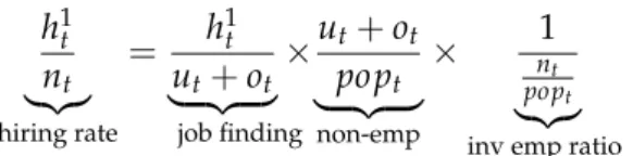
The emerging picture from Figures 1-3 and Tables 2-4 is consistent with some well-known facts. Note that the hiring rate is the product of the job finding rate, the non-employment rate and the inverse of the non-employment rate:

h1_t nt |{z} hiring rate = h 1 t ut+ot | {z } job finding ut+ot popt | {z } non-emp 1 nt popt |{z}

inv emp ratio

(19)

whereuis unemployment, ois the out of the labor force pool and popis the working

age population.

The following table shows the co-movement statistics for these variables.

Table 6

The job finding rate h1t

ut+ot is pro-cyclical, as is well known. The latter feature has

been emphasized by Shimer (2012). The non-employment rate ut+ot

popt and the inverse of

the employment ratio _nt1

popt

are counter-cyclical, as widely known too. At the same time

the gross hiring rate h1t

nt is cyclical, as shown above. The hiring rate is

counter-cyclical as the counter-counter-cyclicality of the last two variables dominates the pro-counter-cyclicality

of the job-finding rate.6

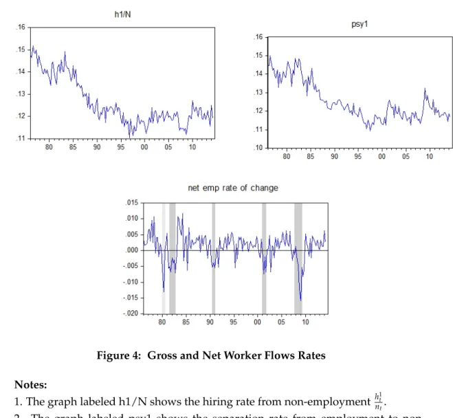
Also note the following. Employment dynamics are given by: nt+1 nt nt = h 1 t nt ψ1_t (20)

Along the cycle the variables in (20) can be shown as follows:

Figure 4

Evidently, in the shaded NBER-dated recession periods, net employment growth is negative with separations being higher than hires. At the same time, in cyclical terms, Figure 5 shows that both rates increase – relative to the HP trend – during recessions, i.e., both are counter-cyclical.

Figure 5

6_{In this context the following quote from Shimer (2012, page 145) is pertinent: “Still, it is most} impor-tant point to recognize the differential behavior of the job finding probability and the number of workers finding jobs;...”

5

Methodology and Data

In order to be empirically evaluated, the afore-going optimality equations of the firm will be estimated. I discuss the data, the estimation methodology and a post-estimation approximation and variance decomposition.

5.1 Data

The data are quarterly and pertain to the private sector of the U.S. economy. For a large part of the empirical work reported below the sample period is 1994-2013. The start

date of 1994 is due to the lack of availability of job to job worker flows (h2_t) data prior

to that. For another part of the empirical work, the sample covers 1976-2013 and the 1976 start is due to the availability of credible monthly CPS data, from which the gross

hiring flows (h1_t) series is derived. This longer sample period covers five NBER-dated

recessions, and both sample periods include the Great Recession (2007-2009) and its aftermath (2009-2013). The data include NIPA data on the NFCB GDP and its deflator, capital, investment, the price of investment goods and depreciation, BLS CPS data on employment and on worker flows, and Fed data computations on tax and depreciation allowances. Appendix C elaborates on the sources and on data construction. These data have the following distinctive features: (i) they pertain to the U.S. private sector;

(ii) both hiringhtand investmentitrefer to gross flows; likewise, separation of workers

ψ_tand depreciation of capitalδtare gross flows; (iii) the estimating equations take into

account taxes and depreciation allowances. Table 7 presents key sample statistics.

Table 7

5.2 Estimation

I use the different model specifications discussed above. For the production function I

use a standard Cobb-Douglas formulation, with productivity shockzt:

f(zt,nt,kt) =eztntαk1_t α, 0<α<1. (21)

The costs functiong was spelled out above (see equation (16)). Estimation pertains to

the parametersα;e1,e2,e31,e32;η₁,η₂,η₃₁,η₃₂,λ1,λ2, or to a sub-set of these parameters.

Estimation of the parameters in the production and costs functions allows for the

quantification of the derivatives git andgvt that appear in the firms’ optimality

as-sociated equation (14) – using Hansen’s (1982) generalized method of moments (GMM). The moment conditions estimated are those obtained under rational expectations. I re-port the J-statistic test of the over-identifying restrictions. I formulate the equations

in stationary terms by dividing the investment equation by ft

kt and the vacancy/hiring

equation by ft

nt. Appendix B spells out the first derivatives included in these equations

and the estimating equations. Importantly, I check whether the estimated g function

fulfills the convexity requirement.

Note that the ideal case would be unconstrained estimation of the power

parame-tersη₁,η₂,η₃₁,η₃₂, of the scale parameterse1,e2,e31ande32, and of the weights included

in the second term, capturing recruiting,λ1andλ2. Attempting to do that, the

estima-tion procedure did not converge. Hence constraints were imposed, and four

parame-ters were freely estimated. Yashiv (2016) tried various configurations ofη₁,η₂,η₃₁,η₃₂

estimation and reported the best ones. Following the results – see Table 2 (page 196) –

the powers were set at η₁ = η₂ = 2 andη₃₁ = η₃₂ = 1. Note that placing such

con-straints on the powers is quite prevalent; often quadratic costs and linear interactions

are simply assumed. The scale parameters(e1,e2,e31,e32)were freely estimated and are

reported in Table 8 below. As to the parametersλ1andλ2, the following procedure was

followed: (i) learning from past studies provided restrictions on the parameter space; and (ii) within this restricted space, fixed values were run and compared. I elaborate on each of these last two points in turn.

Regarding point (i), micro estimates using Swiss data reported in Blatter et al (2016, Table 1) and structural macro estimates using U.S. data in Furlanetto and Groshenny (2016, Table 3), Swedish data in Christiano, Trabandt, and Walentin (2011, p.2039), and Israeli data in Yashiv (2000, Table 2), show that vacancy posting costs are small com-pared to other components of hiring costs, particularly to training costs. Indeed, Chris-tiano, Trabandt, and Walentin (2011), using Bayesian estimation of a DSGE model of Sweden, conclude, in this same context, that “employment adjustment costs are a func-tion of hiring rates, not vacancy posting rates.” These studies then call for a low value

of 1 λ1 λ2. Following them, values of 0 (1 λ1 λ2) 0.3 were examined.

As to point (ii), within the above restricted space, different values ofλ1andλ2were

tried. Empirical success was judged using the same criteria employed throughout: the J statistic test, convexity of the costs function (recalling that the second order conditions depend on the interaction terms), and getting cost estimates that are not large (see the discussion in Sub-section 6.1 below).

Using these two steps, the values of λ1 = 0.6,λ2 = 0.2 were obtained. A similar

5.3 Post Estimation Approximation and Variance Decomposition

Post estimation I compute an approximated present value,QN

t and its variance

decom-position. Iterating forward the RHS of (15) one gets:

PVt = ∞

∑

∏

∏

Following Cochrane (1992), I use the following first-order Taylor expansion to get

(see Appendices D and E for details7):

PVt =Et " ∞

∑

∑

∑

∑

Using a sample period truncated atT, yields the variance decomposition:

var(PVt) = Ω r_Ωf_E(MP) 1 Ω T

∑

∑

∑

∑

The variance of job values breaks down into terms relating to future discount rates

(gr_t+j), productivity growth (g_tf_+j), separation rates (gs_t+j) and marginal profits (MPt+j).

In what follows I look at the relative size of the different terms on the RHS of equation (25) in order to gauge their relative importance.

6

Results

I present GMM estimates of equations (14) and (15) under the alternative specifications described above. Subsequently I use the estimates to present the variance decomposi-tion defined in equadecomposi-tion (25) and a graphical illustradecomposi-tion of key reladecomposi-tionships as implied by estimation.

I use three criteria to evaluate the estimates:

a. The J-statistic test of the over-identifying restrictions.

b. Fulfillment of the convexity requirement for the costs functiong.

invest-ment equations estimated in the q-literature, some specifications imply very high costs. These are deemed to be unreasonable.

6.1 FOC Estimation

Table 8 reports the results of estimation. The table reports the point estimates and their standard errors, Hansen’s (1982) J-statistic and its p-value, noting that some of the spec-ifications estimated were also reported in Yashiv (2016). Table 9 shows the moments of the estimated marginal costs series.

Tables 8 and 9

Row (a) examines a quadratic function (η₁ =η₂=2) with linear interactions (η₃₁ =

η₃₂ =1).8The weights on the different elements of the hiring process – vacancies, hiring

from non-employment, and hiring from other employment – are expressed by the fixed

parametersλ1 = 0.6,λ2 = 0.2, obtained after some experimentation. The parameters

estimated are the scale parameters (e1,e2,e31ande32)of the frictions function (16) and

the labor share (α)of the production function (21). The J-statistic has a high p-value, the

parameters are precisely estimated, and the resulting g function fulfills all convexity

requirements; the estimate of αis around the conventional estimate of 0.66. Table 9

indicates very moderate costs estimates.

Row (b) takes up a very similar specification but ignores job to job flows, i.e., sets

λ2 = e32 =0 andh2t =ψ2t =0. This allows for the use of a much longer data sample –

1976:1-2013:4, with 152 quarterly observations. It too yields a J-statistic with a high

p-value, is, for the most part, precisely estimated, and the resultinggfulfills all convexity

requirements.

The two rows – (a) and (b) - yield similar results in terms of the implied costs re-ported in Table 9. In particular, both feature negative coefficients for the interaction terms, implying complementarity between hiring and investment.

Row (c) follows standard Tobin’s q type of models applied to the hiring of labor and looks at a quadratic specification, ignoring the other factor of production (here ignoring

investment in capital). It thus setsη₂=2,e1 =e31 =e32 =0, i.e., has quadratic vacancy

and hiring costs, with no role for capital (see equation (17)). While there is no rejection of the model, this specification implies very high, unreasonable costs, as seen in Table 9. This is reminiscent of the results in the literature on Tobin’q models for investment.

Row (d) reports the results of the standard (Pissarides-type) search and matching model formulation with linear vacancy costs and no other arguments, as formulated in

equation (18), such thatη₂ = 1,e1 = e31 = e32 = λ1 = λ2 = 0. The emerging estimates

imply even higher costs (shown in Table 9) and the parameterαis estimated at a high

value (0.77).

To see these results in context note the following findings. Mortensen and Nagypal (2006, page 30) note that “Although there is a consensus that hiring costs are important, there is no authoritative estimate of their magnitude. Still, it is reasonable to assume that in order to recoup hiring costs, the firm needs to employ a worker for at least two to three quarters. When wages are equal to their median level in the standard model

(w= 0.983), hiring costs of this magnitude correspond to less than a week of wages.”

The widely-cited Shimer (2005) paper calibrates these costs at c_q = 0.16 using a linear

cost function, which is equivalent to 3.4 weeks of wages. Hagedorn and Manovskii (2008) decompose this cost into two components: (i) the capital flow cost of posting a vacancy; they compute it to be – in steady state – 47.4 percent of the average weekly labor productivity; (ii) the labor cost of hiring one worker, which, relying on micro-evidence, they compute to be 3 percent to 4.5 percent of quarterly wages of a new hire. The first component would correspond to a figure of 0.037 here; the second component would correspond to a range of 0.02 to 0.03 in the terms used here; together this implies 0.057 to 0.067 in current terms or around 1.1 to 1.3 weeks of wages. Blatter et al (2016) survey the micro literature and report estimates of hiring costs ranging between 25% and 131% of quarterly wages, i.e. between 3. 25 and 17 weeks of wages.

The estimates for the preferred specification, i.e., the GMM results reported in row (a) of Table 8 and the first column of Table 9, pertain to marginal costs with a convex costs function, while most of the above pertain to average costs, usually with a linear

function. The preferred specification here has an estimate of(1 τt) gvt

qt_ntft

which is 0.12

at its sample average; given thatwt

ft nt

=0.62 on average, this is the equivalent of 2.5 weeks

of wages. In light of the cited numbers, this is at the low end of the range of macro and micro estimates. The Tobin-q model and the standard model yield the equivalent of 19 and 20 weeks of wages, which are far above the estimates in the literature.

The estimates of marginal investment costs, implied by the preferred specification of

row (a) in Table 8, are on average git

ft kt

=0.53. This estimate is equivalent to an addition

of 3% to the price of a unit of capital. In other words, for every dollar spent on the marginal unit of capital purchased, the firm adds 3 cents in adjustment costs. This result can be compared to the q-literature. One can divide the results in this literature

into three sets: (i) the earlier studies, from the 1980s, suggested high costs, whereby marginal costs range between 3 to 60 in the above terms (average output per unit of capital) and the implied total costs range between 15% to 100% of output; (ii) more recent studies which have reported moderate costs, whereby marginal costs are around 1 in the same terms of average output per unit of capital, and total costs range between 0.5% to 6% of output; (iii) micro-based studies, using cross-sectional or panel data, which have reported low costs, with marginal costs at 0.04 to 0.50 of average output per unit of capital and total costs range between 0.1% to 0.2% of output. The current results are at the high end of the third, low-costs set.

In what follows I denote the results of row (a) as the preferred specification, noting that row (b) yields a similar picture over a longer sample period. I focus on row (a) so as to continue to take into account job to job flows, available only from 1994.

6.2 Post Estimation: Approximation and Variance Decomposition

Table 10 reports the results of the variance decomposition defined by equation (25)

following the approximation equation (23).9

Table 10

For the preferred specification, Table 10 shows that the key determinant of job value

volatility (denotedvar(PVt))is the last term, i.e., the sum of the co-variances of job

val-ues with future marginal profits

T

∑

j=1

(Ω)j 1cov(PVt,MPt+j). Recall that marginal profits

MP_t+j are net marginal productivity less the wage, i.e., 1 τt+j α

g_nt+j ft+j nt+j wt+j ft+j nt+j ) ! .

With the small variability ofτt+j and

g_nt+j

ft+j nt+j

, the main driver of volatility are the future

labor shares wt+j

ft+j nt+j

. All other terms in the decomposition play a very small role.

For the Tobin’q specification and for the standard search and matching model, Table 10 shows that there is some role in the variance decomposition also for the discount rate, the productivity growth rate and the separation rate. Together they account for about 20% of the variance of the approximated, truncated present value, as compared to less than 2% in the preferred specification. This difference helps explain some further implications of the estimates, discussed below.

9_{Experimentation with different values for the truncated horizon shows that starting withT=30 there} is almost no change in the resultingPV(but asTrises the series is shortened). Hence the latter value was chosen to be reported.

6.3 Implications for Key Relationships

I look at the implications of the preferred specification for key relationships in the

model. One such relationship is that of vacancy rates (vt

nt) with job values (

QNt ft nt

) and

investment rates (it

kt). Using equation (12) and the estimates of row (a) in Table 8 this is

given by: vt nt = QN_t ft nt (q1 t+q2t) (1 τt) e31q 1 t +e32q2t kitt e2 (1 λ1 λ2) +λ1q1t +λ2q2t 2 (26)

This equation is plotted in Figure 6.10

Figure 6

This is a linear relationship, whereby labor recruiting, as expressed by the vacancy rate, rises with job values and with the other firm activity – the capital investment rate. In the following sections I look at the cyclical behavior and volatility of these three key

variables – vt nt, QN t ft nt and it kt.

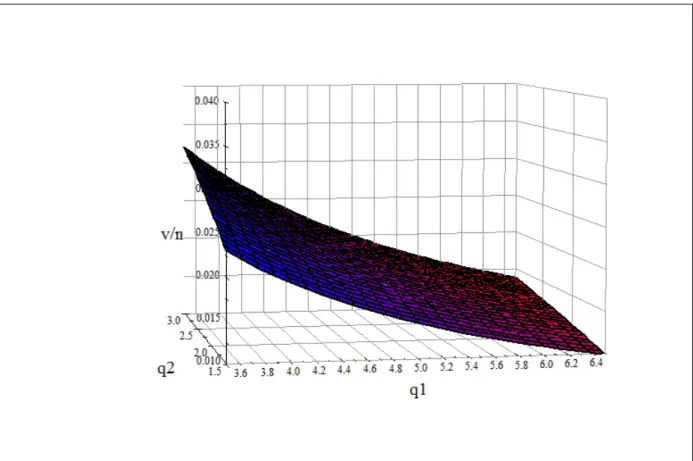
Another such relationship is the one between vacancy rates (vt

nt) and the job filling

rates (q1

t,q2t) which the firm faces. These job-filling rates express the influence of

match-ing processes and market conditions, taken as given by the firm. This is shown in Figure 7.11

Figure 7

This is a non-linear relationship. The figure shows a non-trivial asymmetry: recruit-ing (vt

nt)falls as the job filling rate from non-employment (q

1

t) rises, andrisesas the job

filling rate from other firms (q2_t) rises. Why so? Each job filling rate has three effects.

One is to increase the job value,12thereby increasing the vacancy rate. A second is to

10_{The figure uses the sample averages of tax rates (}

τt) and job filling rates (q1t,q2t) and employs the point estimates of the preferred specification. The figure uses empirically-relevant ranges for vt

nt, shown on the vertical axis, and QNt

ft nt

and it

kt, shown on the horizontal axes.

11_{The figure uses equation (26), the estimates of row (a) in Table 8, and the sample averages of} τt,Q N t ft nt and it kt

12_{Referring to the term} QN_t ft nt (q1 t+q2t) (1 τt) .

reduce marginal costs via the interaction with the rate of investment,13which also op-erates to increase the vacancy rate. The third is a scale effect that raises marginal costs

for any given level of the vacancy rate.14This third effect operates to lower the vacancy

rate. The estimation results of the preferred specification imply that the third effect

dominates in the case of the job filling rate from non-employment (q1_t) and that the first

two effects dominate in the case of the job filling rate from other firms (q2

t).

7

The Cyclicality of Job Values

Section 5 above has presented the cyclical properties of the keydataseries. This section

examines the cyclical properties ofestimatedjob values in the different models.

Table 11 reports the cyclical behavior of estimated job values, using the point es-timates of the LHS of equation (15), i.e., of marginal hiring costs, as reported in the different specifications of Table 8. Figure 8 presents the time series plots of these mar-ginal costs (with the left scale measuring the benchmark and constrained models and the right scale the other two models).

Table 11 and Figure 8

The preferred specification (row (a) of Table 8) indicates counter-cyclicality, the con-strained specification (row (b) of Table 8) weak counter-cyclicality, the Tobin’s q model is weakly pro-cyclical (row (c) of Table 8), while the standard model (row (d) of Table 8) is strongly pro-cyclical.

Getting back to equation (1) the implications of these results are that they indicate very different views of the cyclicality of job values.

Starting with the specification of row (d) in Table 8, the standard search and match-ing (Pissarides-type) model, note that in its simple form the optimality equation is given by (re-writing equation (18)): (1 τt) e2 qt = Et " ρ_t+1(1 τt+1) 1 ft nt fnt+1 gnt+1 wt+1+ (1 ψt+1) e2 qt+1 ft+1 nt+1 # (27)

This equation has a pro-cyclicalMCton the LHS, as shown in Table 11 and Figure 8.

This is to be expected as it depends inversely on the matching rateqt = h_vt_t, which itself

13_{Referring to the term e}

31q1t+e32q2t kitt, noting thate31,e32<0. 14_{Referring to the terme}

2 (1 λ1 λ2) +λ1q1t+λ2q2t 2

is highly counter-cyclical.

The specification of row (c) in Table 8, the Lucas-Prescott/Tobin approach has mar-ginal costs being weakly pro-cyclical, as seen in Table 11 and Figure 8. Repeating equa-tion (17): (1 τt) e2 qt " (1 λ1 λ2) +λ1q1t+λ2q2t #2 vt nt =Et 1_f t nt " ρ_t+1(1 τt+1) " fnt+1 gnt+1 wt+1 +(1 ψ_t+1)g_qvt+1 t+1 ## (28)

The reason for the weak pro-cyclicality is that the pro-cyclicality of e2

qt and of

vt

nt is

offset to some extent by the counter-cyclicality ofq1_t andq2_t.

The preferred specification of row (a) in Table 8, implies the opposite. The results of Table 11 and Figure 8 indicate counter-cyclicality. Note that this is a broader model. It

follows the Pissarides approach of using a vacancy creation equation butMCtdepends

on all the relevant rates – h1t

nt,

h2

t

nt and

vt

nt. The equation here is:

(1 τt) 1 qt 2 6 6 4 e2 " (1 λ1 λ2) +λ₁q1_t +λ2q2t #2 vt nt +(e31q1t +e32q2t)kitt 3 7 7 5= Et 1 ft nt " ρ_t+1(1 τt+1) " fnt+1 gnt+1 wt+1 +(1 ψ_t+1)g_qvt+1 t+1 ## (29) This model delivers counter-cyclicality on both sides of the equation, as the

pro-cyclicality of _q1

t

vt

nt, and of(e31q

1

t +e32q2t)kitt is out-weighed by the counter-cyclical term

(1 λ1 λ2) +λ1q1t +λ2q2t 2

. Note, two related points:

One is that it is of course not only the LHS of the hiring optimality equation which differ across models, but also their RHS. In equations (27), (28) and (29) above, the

expressions gvt+1

qt+1 differ across models. Note that Table 10 gave evidence of that in terms

of the variance decomposition.

The second is that all three models relate to the present value of marginal profits. One can therefore ask what is the cyclical behavior of this latter present value, and why do the models differ on this aspect. I examine this question in the next section.

In a recent paper, Kudlyak (2014) suggested a related concept she has termed “the user cost” of labor. Comparing this concept to the current one, the following can be shown. The user cost of labor is the sum of two terms:

(i) the first difference in job values, QNt

ft nt

(2014, equation 4) callsUC_tV.

(ii) a term that Kudlyak (2014, equation 2) callsUCW_t and defines as (p.56): “the sum

of the hiring wage in periodtand the expected present value of the differences between

wages paid from the next period onward in the employment relationship that starts in

tand the employment relationship that starts int+1.”

Hence the job value is not the user cost of labor. Two crucial differences emerge between Kudlyak (2014) and this paper:

a. The user costUCtis not the same concept as the job value and not even of its first

difference, as it includes an important other component,UCW

t .

b. Kudlyak (2014) assumes constant discounting, constant separation, no produc-tivity growth, no taxes, and no employment-dependent hiring costs.

This leads to the following key differences in the analysis:

a. The cyclicality ofUCtshould not be expected to be the same as the cyclicality of

QN t ft nt

, which is a key issue in the current paper.

b. The analysis of this paper assigns a role to variable discounting, separation and productivity growth; Table 10 column 4 assigns 16% of the variance of the relevant present value expression – within the framework of the standard search and matching model – to those variables which are assumed constant in Kudlyak (2014).

Moreover, the above holds true for the restricted setting of the standard search and

matching model cost function which hase1 = e31 = e32 = 0,λ1 = λ2 = 0 andη₂ = 1.

The main parts of the current paper deal with the preferred specification of hiring costs, which are richer.

8

The Role of the Labor Share in Job Value Cyclicality

The labor share in GDP plays a key role in the afore-going results. It has also been the focus of some attention in recent macroeconomic models of the business cycle. The main reason for the key results of this paper is its cyclical behavior. The variance

de-composition of the approximated PVt, reported in Table 10 above, has shown that the

key role is played by marginal profits (repeating equation (24)):

MP_t+j 1 τt+j 0 @α gnt+j ft+j nt+j wt+j ft+j nt+j ) 1 A (30)

Asαis constant, the tax rate (τt+j) is fixed over long periods and the term

g_nt+1

ft+1

nt+1

estimated to be small, the main driver is the labor share, wt+1

ft+1

nt+1

.

Consider the cyclicality of the labor share. In Table 12, I present in panel (a) its dynamic correlations with GDP. In panel (b), I present the dynamic correlations with

GDP of an approximated present value of these marginal profits (30), given by:15

PVt(MPt+s) = T

∑

∏

Note that these dynamic correlations, for logged and HP filtered variables, are com-puted using only data, with no parameter estimates.

Table 12

Noting the bolded numbers in panel (a) of the table, dynamically, the labor share is pro-cyclical. As a result the job values it engenders are cyclical. This counter-cyclicality can be seen in panel (b), showing the dynamic correlations of the approxi-mated job value expression in (31) with GDP. It is this dynamic stochastic behavior of the labor share which is the key determinant of counter-cyclical job values.

Note that the different models examined in estimation capture this job value behav-ior differentially, as seen in Section 7 above. There are several reasons for the differ-ences across models: the relevant estimating equations, i.e., the empirical counter-parts

of equations (27), (28) and (29), use data from adjacent periodstandt+1 rather thanT

period ahead data as in equation (31); the empirical equations use actual data variables, not expected ones, and thus contain errors; and the models posit different parametric forms of the cost function (g) and hence constrain the empirical equations in different ways.

The point is that the preferred specification captures the counter-cyclicality of job values shown in Table 12, while the Tobin and standard search and matching models do not.

This cyclical behavior of the labor share has recently been noted by a number of authors in other Macro contexts. The observation, whereby the labor share first falls in a boom and subsequently rises for a substantial period of time, i.e., is dynamically pro-cyclical, was discussed by Rios-Rull and Santaeulalia-Llopis (2010). Hall (2014) finds

15_{There are two aspects to this approximation: it ignores the} gnt+1 ft+1 nt+1

term and it truncates the infinite sum atT.

that the labor share is a-cyclical contemporaneously and pro-cyclical subsequently. Nekarda and Ramey (2013) examine the cyclicality of ups. Essentially they treat the mark-up as the inverse of the labor share (see their equation 5), allowing various modifica-tions to the relamodifica-tionship, such as overhead hours, CES production funcmodifica-tions, and differ-entials between marginal and average wages. Studying both aggregate and four-digit

manufacturing data of the U.S. economy, they find that mark-ups arecontemporaneously

pro-cyclical and thatdynamicallythey are counter-cyclical. The latter finding means that

if GDP is low now (recession), mark-ups will rise henceforth (see their Figure 2). This is

similar to the finding here that job values are counter-cyclical, i.e., that thepresent value

of profits rises in recessions. It is so for the same reason, namely that the future labor share declines (i.e., again, dynamically the labor share is pro-cyclical). These findings are not in contradiction with the findings of other recent papers, such as Haefke,

Son-ntag, and van Rens (2013), whereby the real wagewt itself is contemporaneously and

over some lags and leads pro-cyclical, as this is true for the current paper’s data. Note that the current paper does not discuss a general equilibrium, structural model. It focuses only on the FOC for firm optimal hiring and investment. Inter alia, it takes wage share behavior as given. Therefore it does not attempt to explain the reasons for the dynamic pro-cyclicality of the labor share. But such an explanation may be derived from a structural DSGE setting. Thus, Rios-Rull and Santaeulalia-Llopis (2010) point out that in RBC modelling, in order to account for this pattern of the data, one cannot maintain the assumptions of Cobb Douglas production and competitive factor prices. They point to labor search models as a potential modelling route. In those models, a bargaining protocol for wages, combined with the FOC of the type examined here, breaks the identity of wage and labor productivity behavior. In this set up, following a positive productivity shock, the model may replicate the data: wages rise a bit and then fall slowly, while the average product rises a lot and then monotonically declines; consequently, the labor share first drops and then rises (see their Figure 6 on page 946). A different modelling direction was proposed by Growiec, McAdam and Mu´ckr (2015). They find that in the medium-term the labor share is pro-cyclical, while in the short run it is counter-cyclical. These findings are in line with the current findings. They then offer explanations in terms of an endogenous, R&D-based growth model, with capital and labor augmenting innovations.

Note, too, that the different models examined in estimation capture this job value behavior differentially, as seen in Section 7 above. There are several reasons for the dif-ferences across models: the relevant estimating equations, i.e., the empirical

t+1 rather than T period ahead data as in equation (22); the empirical equations use actual data variables, not expected ones, and thus contain errors; and the models posit different parametric forms of the cost function (g) and hence constrain the empirical equations in different ways. It is this last point which deserves emphasis. The standard

model places the following restrictions: e1 = e31 = e32 = 0,λ1 = λ2 = 0 andη₂ = 1.

Tobin’s Q model places the restrictionse1 = e31 = e32 = 0 andη₂ = 2. It turns out that

the data do not conform these restrictions. The preferred specification, which gives dif-ferential weights to the different recruiting variables (unlike the standard model), and allows for important interactions with investment (unlike the standard model and To-bin’s model), fits the data better. It delivers a “different story,” whereby hiring and job values are counter-cyclical, while the Tobin and standard search and matching models do not, as shown in Table 11.

9

The Volatility of Recruitment Rates

The focus so far has been on the cyclicality of recruiting and of the associated job values.

In this section I turn to study thevolatilityof the key variables expressing recruitment

behavior, using the estimation results. In particular, I seek to explain the finding of high volatility, which has been widely discussed in the literature, mostly following Shimer (2005). The idea is to show that the estimated model not only explains co-movement but is able also to account for high volatility. The connections of co-movement and volatility are then explored.

I start by presenting some pertinent data moments. I then do variance decom-positions of the vacancy rate, the total hiring rate, and the rate of hiring from non-employment using the preferred estimates. I conclude by summarizing the findings with respect to the determinants of the high volatility of these recruitment variables.

9.1 Data Moments

To fix ideas as to the volatility facts to be explained in this section, consider the follow-ing data moments. Table 13a shows the volatility, in terms of the standard deviations,

of the key variables in firm behavior: the hiring rate – both the total one ht

nt and the rate

from non-employment h1t

nt, the vacancy rate

vt

nt, and the job filling rates q

1

t andq2t. I also

look at the investment rate it

kt.

16 _{Table 13b presents the standard deviation and}

corre-16_{The discussion here complements the discussion in Section 4 above. All variables are logged and} HP-filtered.

lation of two key determinants: output (NFCB GDP, ft) and the job value ( Q

N t

(1 τt)_ntft

), as estimated in Table 8 row (a). Table 13c reports the co-movement of the firm variables of Table 13a and the two determinant variables examined in Table 13b.

Tables 13 a,b,c

These series are all shown in Figure 9 with the vertical lines indicating the start and end of NBER-dated recessions.

Figure 9

The following points may be noted:

(i) The vacancy rate and the job filling rates are highly volatile. This a key point to be explained.

(ii) The above rates are much more volatile than the hiring rates. Why so? Noting

that ht

nt = (q

1

t +q2t)vntt, this is the result of the negative co-movement of vacancy rates

vt

nt and job filling rates(q1_t+q2_t).

(iii) Job values are much more volatile than output and are negatively correlated with it, i.e., are countercyclical. The latter feature was emphasized above. In what follows we shall see how this stochastic behavior accounts for volatility.

(iv) In terms of business cycle facts, the well-known moments shown here are the pro-cyclicality of the investment rate and of the vacancy rate and the counter-cyclicality of job filling rates. Much less known is the weak cyclicality of hiring rates, with the rate of hiring from non-employment, actually being counter-cyclical, as discussed in Section 4 above.

(v) Job values have positive co-movement with the worker flow from non-employment,

as expressed by the hiring rateh1t

nt and the job filling rateq

1

t. But they negatively co-move

with the decision variables of the firm – vacancy and investment rates. This feature, too, plays a role in explaining volatility.

These moments suggest differential behavior of the various recruitment variables, which I turn to analyze using variance decompositions.

9.2 The Vacancy Rate

As the analysis is somewhat involved, I break it down into sub-topics.

Deriving The Vacancy Rate in the Estimated Model. To explain the volatility of the

(1 τt) gvt qt_nft_t = Q N t ft nt Using the preferred estimates of Table 8 row (a) I get:

1 q1 t +q2t " e2 (1 λ1 λ2) +λ1q1t +λ2q2t 2 _vt nt + e31q1t +e32q2t kitt # = Q N t (1 τt)_nft_t

The vacancy rate can then be expressed as follows (basically re-writing equation (26)): vt nt = QNt (1 τt)_ntft q1_t +q2_t e2 (1 λ1 λ2) +λ1q1t +λ2q2t 2 (32) e31q1t+e32q2t kitt e2 (1 λ1 λ2) +λ1q1t +λ2q2t 2

Equation (32) shows that the vacancy rate is composed of two terms:

(i) The job value QtN

(1 τt)_ntft , multiplied by a factor (q 1 t+q2t) e2[(1 λ1 λ2)+λ1q1t+λ2q2t] 2 , which is

a non-linear function of the job filling ratesq1

t andq2t and model parameters (e2,λ1,λ2).

(ii) The investment rate it

kt, multiplied by another factor

(e31q1t+e32q2t)

e2[(1 λ1 λ2)+λ1q1t+λ2q2t]

2 ,

which is a (different) non-linear function of the job filling rates q1_t and q2_t and model

parameters (e2,e31,e32,λ1,λ2).

In other words, vacancy rates are driven by job values, and through the interaction of costs, by investment rates, themselves driven by capital values.

Variance Decomposition of the Vacancy Rate. Table 14 reports the following variance