Three-Dimensional Scene Flow

Appeared in the 7th International Conference on Computer Vision, Corfu, Greece, September 1999.

Three-Dimensional Scene Flow

Sundar Vedula

y

, Simon Baker

y

, Peter Rander

yz

, Robert Collins

y

, and Takeo Kanade

y y

The Robotics Institute, Carnegie Mellon University, Pittsburgh, PA 15213

z

Zaxel Systems Inc., Ten 40th Street, Pittsburgh, PA 15201

Abstract

Scene flow is the three-dimensional motion field of points in the world, just as optical flow is the two-dimensional motion field of points in an image. Any optical flow is simply the projection of the scene flow onto the im-age plane of a camera. In this paper, we present a frame-work for the computation of dense, non-rigid scene flow from optical flow. Our approach leads to straightforward linear algorithms and a classification of the task into three major scenarios: (1) complete instantaneous knowledge of the scene structure, (2) knowledge only of correspondence information, and (3) no knowledge of the scene structure. We also show that multiple estimates of the normal flow cannot be used to estimate dense scene flow directly with-out some form of smoothing or regularization.

1

Introduction

Optical flow is a two-dimensional motion field in the image plane. It is the projection of the three-dimensional motion of the world. If the world is completely non-rigid, the motions of the points in the scene may all be indepen-dent of each other. One representation of the scene motion is therefore a dense three-dimensional vector field defined for every point on every surface in the scene. By analogy with optical flow, we refer to this three-dimensional motion field as scene flow.

In this paper, we present a framework for the compu-tation of dense, non-rigid scene flow directly from optical flow. Our approach leads to efficient linear algorithms and a classification of the task into three major scenarios:

1. Complete instantaneous knowledge of the structure of the scene, including surface normals and rates of change of depth maps. In this case, only one optical flow is required to compute the scene flow.

2. Knowledge only of stereo correspondences. In this case, at least two optical flows are needed to compute the scene flow, but more improve robustness.

3. No knowledge of the surface. In this case, several op-tical flows can be used in a reconstruction algorithm to estimate the scene structure (and then scene flow).

For each scenario, we propose an algorithm and demon-strate it on a collection of video sequences of a dynamic, non-rigid scene. We also show that multiple estimates of the normal flow cannot be used to estimate scene flow di-rectly, without some form of regularization or smoothing.

One possible application of scene flow is as a predictor for efficient and robust stereo. Given a reconstructed model of the scene at a certain time, one would like to obtain an estimate of the structure at the next time step using minimal computation. This would allow: (1) more efficient compu-tation of the structure at the next time step because a first estimate would be available to reduce the search space, and (2) more robust computation of the structure because the predicted structure can be integrated with the new stereo data. Other applications of scene flow include various dy-namic rendering and interpretation tasks, from the genera-tion of slow-mogenera-tion replays, to the understanding and mod-eling of human actions.

1.1 Related Work

Computing the three-dimensional motion of a scene is a fundamental task in computer vision that has been ap-proached in a wide variety of ways. If the scene is rigid and the cameras are calibrated, the three-dimensional scene structure and relative motion can be computed (up to a scale factor) from a single monocular video sequence using

structure-from-motion [Ullman, 1979]. If the scene is only

piecewise rigid, extensions to structure-from-motion algo-rithms can be used. See, for example, [Zhang and Faugeras, 1992a] and [Costeira and Kanade, 1998].

Although restricted forms of non-rigidity can be ana-lyzed using the structure-from-motion paradigm [Avidan and Shashua, 1998], general non-rigid motion cannot be estimated from a single camera without additional assump-tions about the scene. However, given strong enough a

priori assumptions about the scene, for example in the

form of a deformable model [Pentland and Horowitz, 1991] [Metaxas and Terzopoulos, 1993] or the assumption that the motion minimizes the deviation from a rigid body mo-tion [Ullman, 1984], recovery of three-dimensional non-rigid motion from a monocular view is possible. See [Penna, 1994] for a recent survey of monocular non-rigid 722

motion estimation, and the assumptions used to compute it. Another common approach to recovering three-dimensional motion is to use multiple cameras and com-bine stereo and motion in an approach known as

motion-stereo. Nearly all motion-stereo algorithms assume that

the scene is rigid. See, for example, [Waxman and Dun-can, 1986], [Young and Chellappa, 1999], and [Zhang and Faugeras, 1992b]. A paper which explicitly combines two optical flow fields is that of [Shi et al., 1994]. In this paper, both the analysis and implementation are only applicable to certain simple motions of the camera (i.e. translations).

A few motion-stereo papers do consider non-rigid mo-tion, including [Liao et al., 1997] and [Malassiotis and Strintzis, 1997]. The former uses a relaxation-based al-gorithm to co-operatively match features in both the tem-poral and spatial domains. It therefore does not provide dense motion. The latter uses a grid which acts as a de-formable model in a generalization of the monocular ap-proaches mentioned above. Besides requiring a priori models of the scene, most deformable-model based ap-proaches to motion-stereo would be too inefficient for our stereo-prediction application.

2

Image Formation Preliminaries

Consider a non-rigidly moving surfacef(x;y ;z;t)=0

imaged by a fixed camerai, with34projection matrix

P

i, as illustrated in Figure 1. There are two aspects to the

formation of the image sequenceI i =I i (u i ;v i ;t)captured

by camerai: (1) the relative camera and surface geometry,

and (2) the illumination and surface photometrics.

2.1 Relative Camera and Surface Geometry

The relationship between a point(x;y ;z)on the surface

and its image coordinates(u i

;v

i

)in cameraiis given by: u i = [

P

i ] 1 (x;y ;z;1) T [

P

i ] 3 (x;y ;z;1) T (1) v i = [

P

i ] 2 (x;y ;z;1) T [

P

i ] 3 (x;y ;z;1) T (2) where[

P

i ] j is the j th

row of

P

i. Equations (1) and (2)

describe the mapping from a point

x

= (x;y ;z)on the

surface to its image

u

i = (u

i ;v

i

)in camera i. Without

knowledge of the surface, these equations are not invert-ible. Givenf, they can be inverted, but the inversion

re-quires intersecting a ray in space with the surfacef.

The differential relationships between

x

and

u

i can be

represented by a23Jacobian matrix @ui

@x

. The 3 columns of the Jacobian matrix store the differential change in pro-jected image co-ordinates per unit change inx,y, andz. A

closed-form expression for @ui @x

as a function of

x

can be derived by differentiating Equations (1) and (2) symboli-cally. The Jacobian @ui

@x

describes the relationship between a small change in the point on the surface and its image in

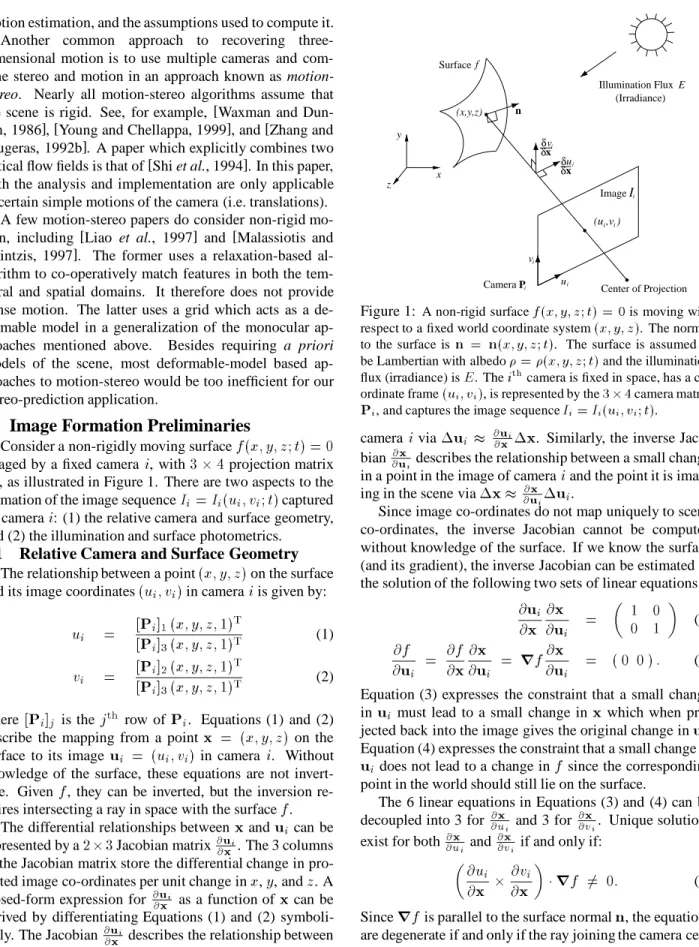
ui vi ui δ δx vi x δ δ (u ,v )i i Illumination Flux E (Irradiance) 00 11 0 0 1 1 00 11 n (x,y,z) Camera Pi Image i f Surface I Center of Projection z x y

Figure 1: A non-rigid surfacef(x;y ;z;t)=0is moving with

respect to a fixed world coordinate system(x;y ;z). The normal

to the surface is n = n(x;y ;z;t). The surface is assumed to

be Lambertian with albedo=(x;y ;z;t)and the illumination

flux (irradiance) isE. Thei

th

camera is fixed in space, has a

co-ordinate frame(u

i ;v

i

), is represented by the34camera matrix

Pi, and captures the image sequenceIi=Ii(ui;vi;t).

cameraivia

u

i

@ui

@x

x

. Similarly, the inverse

Jaco-bian @x @ui

describes the relationship between a small change in a point in the image of cameraiand the point it is

imag-ing in the scene via

x

@x

@ui

u

i.

Since image co-ordinates do not map uniquely to scene co-ordinates, the inverse Jacobian cannot be computed without knowledge of the surface. If we know the surface (and its gradient), the inverse Jacobian can be estimated as the solution of the following two sets of linear equations:

@

u

i @

x

@

x

@

u

i = 1 0 0 1 (3) @f @

u

i = @f @

x

@

x

@

u

i = rf @

x

@

u

i = (0 0): (4)

Equation (3) expresses the constraint that a small change in

u

i must lead to a small change in

x

which when

pro-jected back into the image gives the original change in

u

i.

Equation (4) expresses the constraint that a small change in

u

idoes not lead to a change in

f since the corresponding

point in the world should still lie on the surface.

The 6 linear equations in Equations (3) and (4) can be decoupled into 3 for @x

@ui

and 3 for @x @vi

. Unique solutions exist for both @x

@u

i

and@x @v

i

if and only if:

@u i @

x

@v i @

x

rf 6= 0: (5)

Sincerfis parallel to the surface normal

n

, the equations

are degenerate if and only if the ray joining the camera cen-ter of projection and

x

is tangent to the surface.

2.2 Illumination and Surface Photometrics

At a point

x

in the scene, the irradiance or illumination flux measured in the direction

m

at timet can be

repre-sented byE =E(

m

;

x

;t)[Horn, 1986]. This 6D

irradi-ance functionEis what is described as the plenoptic

func-tion in [Adelson and Bergen, 1991].

We denote the net directional irradiance of light at the point(x;y ;z)on the surface at timetby

s

=

s

(x;y ;z;t).

The net directional irradiance

s

is a vector quantity and is given by the (vector) surface integral of the irradianceE

over the visible hemisphere of possible directions:

s

(x;y ;z;t) = Z

S(n)

E(

m

;x;y ;z;t)d

m

(6)

whereS(

n

)=f

m

: k

m

k=1and

m

n

0gis the

hemi-sphere of directions from which light can fall on a surface patch with surface normal

n

.

We assume that the surface is Lambertian with albedo

= (

x

;t). Then, assuming that the point

x

=(x;y ;z)

is visible in thei th

camera, and that the intensity registered in imageI

iis proportional to the radiance of the point that

it is the image of (i.e. image irradiance is proportional to scene radiance [Horn, 1986]), we have:

I

i (

u

i

;t) = ,C(

x

;t)[

n

(

x

;t)

s

(

x

;t)] (7)

whereCis a constant that only depends upon the diameter

of the lens and the distance between the lens and the image plane. The image pixel

u

i

=(u

i ;v

i

)and the surface point

x

=(x;y ;z)are related by Equations (1) and (2).

3

Two-Dimensional Optical Flow

Suppose

x

(t)is the 3D path of a point on the surface

and the image of this point in camera iis

u

i

(t). The 3D

motion of this point is dx dt

and the 2D image motion of its projection is dui

dt

. The 2D flow fielddui dt

is usually known as optical flow. As the point

x

(t)moves on the surface, it

is natural to assume that its albedo=(

x

(t);t)remains

constant; i.e. we assume that

d

dt

= 0: (8)

(For a deformably moving surface, it is only the surface properties like albedo that distinguish points anyway). The basis for optical flow algorithms is then the equation:

dI i dt = rI i d

u

i dt + @I i @t = ,C(

x

;t) d dt [

n

s

] (9) whererI

i is the spatial gradient of the image, dui

dt

is the optical flow, and @Ii

@t

is the instantaneous rate of change of the image intensityI

i =I i (

u

i ;t).

The term

n

s

depends upon both the shape of the surface

(

n

) and the illumination (

s

). To avoid explicit dependence

upon the structure of the three-dimensional scene, it is often assumed that:

n

s

= Z S(n) E(

m

;

x

;t)

n

d

m

(10) is constant (d dt

[

n

s

] =0). With uniform illumination or

a surface normal that does not change rapidly, this assump-tion holds well (at least for Lambertian surfaces).

In either scenario dIi dt

goes to zero, and we arrive at the

Normal Flow or Gradient Constraint Equation, used by

“differential” optical flow algorithms [Barron et al., 1994]:

rI i d

u

i dt + @I i @t = 0: (11)

Using this constraint, a large number of algorithms have been proposed for estimating the optical flow du

i

dt

. See [Barron et al., 1994] for a recent survey.

4

Three-Dimensional Scene Flow

In the same way that optical flow describes an instanta-neous motion field in an image, we can think of scene flow as a three-dimensional flow field dx

dt

describing the motion at every point in the scene. The analysis in Section 2.1 was only for a fixed timet. Now suppose there is a point

x

=

x

(t)moving in the scene. The image of this point in

cameraiis

u

i

=

u

i

(t). If the camera is not moving, the

rate of change of

u

iis uniquely determined as: d

u

i dt = @

u

i @

x

d

x

dt : (12)

Inverting this relationship is, again, impossible with-out knowledge of the surfacef. To invert it, note that

x

depends not only on

u

i, but also on the time, indirectly

through the surfacef =f(

x

;t). That is

x

=

x

(

u

i

(t);t).

Differentiating this expression with respect to time gives:

d

x

dt = @

x

@

u

i d

u

i dt + @

x

@t ui : (13)

This equation says that the motion of a point in the world is made up of two components. The first is the projection of the scene flow on the plane tangent to the surface and pass-ing through

x

. This is obtained by taking the instantaneous motion on the image plane (the optical flow dui

dt

), and pro-jecting it out into the scene using the inverse Jacobian @x

@ui

. The second term is the contribution to scene flow arising from the three-dimensional motion of the point in the scene imaged by a fixed pixel. It is the instantaneous motion of

x

along the ray corresponding to

u

i. The magnitude of @x @t u i

is (proportional to) the rate of change of the depth of the surfacef along this ray. A derivation of

@x @t u i is presented in Appendix A.

There are three major ways of computing scene flow, de-pending upon what is known about the scene at that instant:

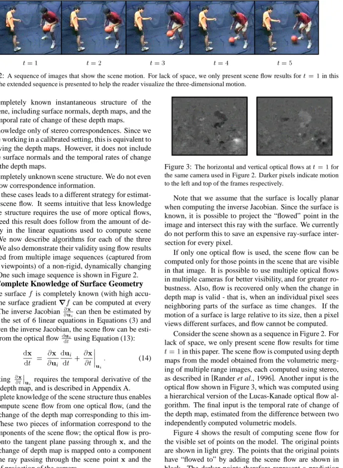
Figure 2: A sequence of images that show the scene motion. For lack of space, we only present scene flow results fort=1in this

paper. The extended sequence is presented to help the reader visualize the three-dimensional motion.

1. Completely known instantaneous structure of the scene, including surface normals, depth maps, and the temporal rate of change of these depth maps.

2. Knowledge only of stereo correspondences. Since we are working in a calibrated setting, this is equivalent to having the depth maps. However, it does not include the surface normals and the temporal rates of change of the depth maps.

3. Completely unknown scene structure. We do not even know correspondence information.

Each of these cases leads to a different strategy for estimat-ing the scene flow. It seems intuitive that less knowledge of scene structure requires the use of more optical flows, and indeed this result does follow from the amount of de-generacy in the linear equations used to compute scene flow. We now describe algorithms for each of the three cases. We also demonstrate their validity using flow results computed from multiple image sequences (captured from various viewpoints) of a non-rigid, dynamically changing scene. One such image sequence is shown in Figure 2.

4.1 Complete Knowledge of Surface Geometry

If the surface f is completely known (with high

accu-racy), the surface gradientrf can be computed at every

point. The inverse Jacobian @x @u

i

can then be estimated by solving the set of 6 linear equations in Equations (3) and (4). Given the inverse Jacobian, the scene flow can be esti-mated from the optical flow dui

dt using Equation (13): d

x

dt = @

x

@

u

i d

u

i dt + @

x

@t ui : (14) Computing @x @t u i

requires the temporal derivative of the surface depth map, and is described in Appendix A.

Complete knowledge of the scene structure thus enables us to compute scene flow from one optical flow, (and the rate of change of the depth map corresponding to this im-age.) These two pieces of information correspond to the two components of the scene flow; the optical flow is pro-jected onto the tangent plane passing through

x

, and the rate of change of depth map is mapped onto a component along the ray passing through the scene point

x

and the center of projection of the camera.

Figure 3: The horizontal and vertical optical flows att=1for

the same camera used in Figure 2. Darker pixels indicate motion to the left and top of the frames respectively.

Note that we assume that the surface is locally planar when computing the inverse Jacobian. Since the surface is known, it is possible to project the “flowed” point in the image and intersect this ray with the surface. We currently do not perform this to save an expensive ray-surface inter-section for every pixel.

If only one optical flow is used, the scene flow can be computed only for those points in the scene that are visible in that image. It is possible to use multiple optical flows in multiple cameras for better visibility, and for greater ro-bustness. Also, flow is recovered only when the change in depth map is valid - that is, when an individual pixel sees neighboring parts of the surface as time changes. If the motion of a surface is large relative to its size, then a pixel views different surfaces, and flow cannot be computed.

Consider the scene shown as a sequence in Figure 2. For lack of space, we only present scene flow results for time

t=1in this paper. The scene flow is computed using depth

maps from the model obtained from the volumetric merg-ing of multiple range images, each computed usmerg-ing stereo, as described in [Rander et al., 1996]. Another input is the optical flow shown in Figure 3, which was computed using a hierarchical version of the Lucas-Kanade optical flow al-gorithm. The final input is the temporal rate of change of the depth map, estimated from the difference between two independently computed volumetric models.

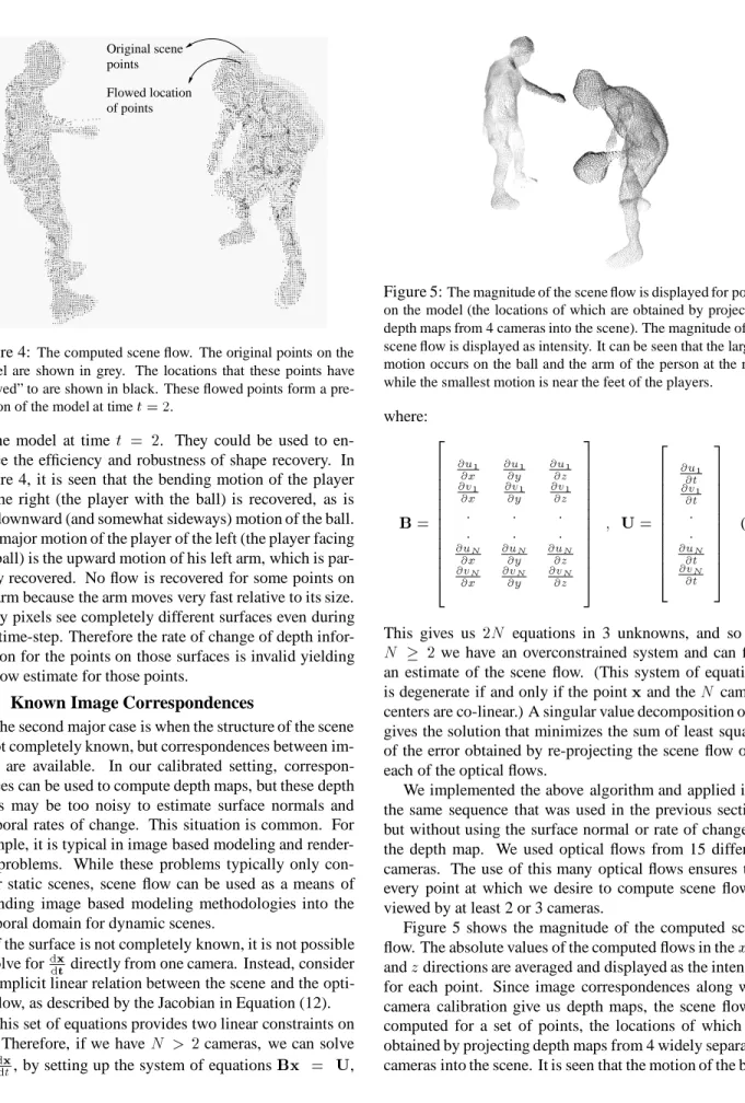
Figure 4 shows the result of computing scene flow for the visible set of points on the model. The original points are shown in light grey. The points that the original points have “flowed to” by adding the scene flow are shown in black. The darker points therefore represent a prediction

Flowed location of points points Original scene

Figure 4: The computed scene flow. The original points on the model are shown in grey. The locations that these points have “flowed” to are shown in black. These flowed points form a

pre-diction of the model at timet=2.

of the model at time t = 2. They could be used to

en-hance the efficiency and robustness of shape recovery. In Figure 4, it is seen that the bending motion of the player on the right (the player with the ball) is recovered, as is the downward (and somewhat sideways) motion of the ball. The major motion of the player of the left (the player facing the ball) is the upward motion of his left arm, which is par-tially recovered. No flow is recovered for some points on the arm because the arm moves very fast relative to its size. Many pixels see completely different surfaces even during one time-step. Therefore the rate of change of depth infor-mation for the points on those surfaces is invalid yielding no flow estimate for those points.

4.2 Known Image Correspondences

The second major case is when the structure of the scene is not completely known, but correspondences between im-ages are available. In our calibrated setting, correspon-dences can be used to compute depth maps, but these depth maps may be too noisy to estimate surface normals and temporal rates of change. This situation is common. For example, it is typical in image based modeling and render-ing problems. While these problems typically only con-sider static scenes, scene flow can be used as a means of extending image based modeling methodologies into the temporal domain for dynamic scenes.

If the surface is not completely known, it is not possible to solve fordx

dt

directly from one camera. Instead, consider the implicit linear relation between the scene and the opti-cal flow, as described by the Jacobian in Equation (12).

This set of equations provides two linear constraints on

dx

dt

. Therefore, if we haveN > 2cameras, we can solve

for dx dt

, by setting up the system of equations

Bx

=

U

,

Figure 5:The magnitude of the scene flow is displayed for points on the model (the locations of which are obtained by projecting depth maps from 4 cameras into the scene). The magnitude of the scene flow is displayed as intensity. It can be seen that the largest motion occurs on the ball and the arm of the person at the rear, while the smallest motion is near the feet of the players.

where:

B

= 2 6 6 6 6 6 6 6 6 6 6 6 4 @u 1 @x @u 1 @y @u 1 @z @v1 @x @v1 @y @v1 @z : : : : : : @u N @x @u N @y @u N @z @vN @x @vN @y @vN @z 3 7 7 7 7 7 7 7 7 7 7 7 5 ;

U

= 2 6 6 6 6 6 6 6 6 6 6 4 @u1 @t @v1 @t : : @u N @t @v N @t 3 7 7 7 7 7 7 7 7 7 7 5 (15)

This gives us 2N equations in 3 unknowns, and so for N 2we have an overconstrained system and can find

an estimate of the scene flow. (This system of equations is degenerate if and only if the point

x

and theN camera

centers are co-linear.) A singular value decomposition of

B

gives the solution that minimizes the sum of least squares of the error obtained by re-projecting the scene flow onto each of the optical flows.

We implemented the above algorithm and applied it to the same sequence that was used in the previous section, but without using the surface normal or rate of change of the depth map. We used optical flows from 15 different cameras. The use of this many optical flows ensures that every point at which we desire to compute scene flow is viewed by at least 2 or 3 cameras.

Figure 5 shows the magnitude of the computed scene flow. The absolute values of the computed flows in thex,y,

andzdirections are averaged and displayed as the intensity

for each point. Since image correspondences along with camera calibration give us depth maps, the scene flow is computed for a set of points, the locations of which are obtained by projecting depth maps from 4 widely separated cameras into the scene. It is seen that the motion of the ball,

Flowed location of points Original Scene points

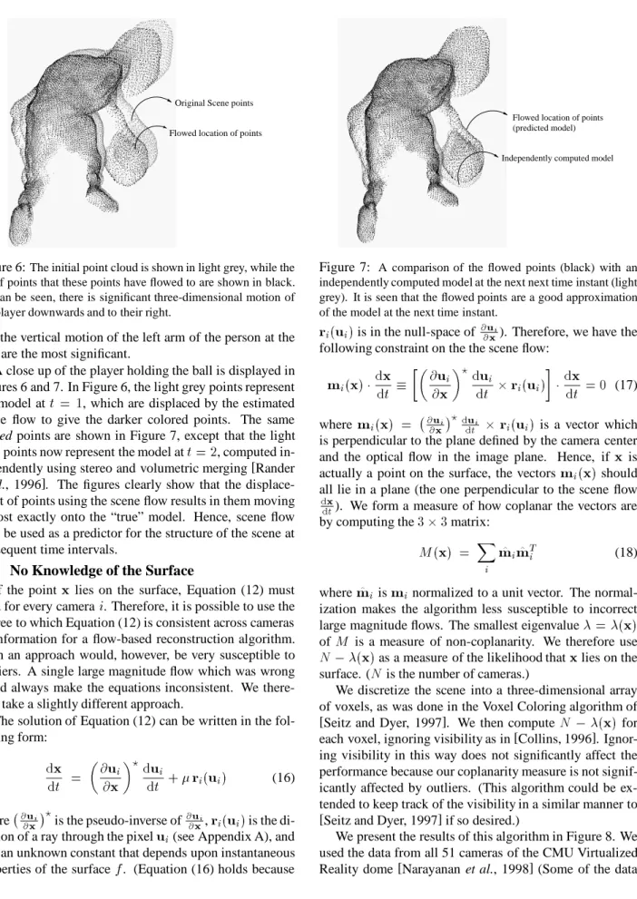
Figure 6:The initial point cloud is shown in light grey, while the set of points that these points have flowed to are shown in black. As can be seen, there is significant three-dimensional motion of the player downwards and to their right.

and the vertical motion of the left arm of the person at the rear are the most significant.

A close up of the player holding the ball is displayed in Figures 6 and 7. In Figure 6, the light grey points represent the model att = 1, which are displaced by the estimated

scene flow to give the darker colored points. The same

flowed points are shown in Figure 7, except that the light

grey points now represent the model att=2, computed

in-dependently using stereo and volumetric merging [Rander

et al., 1996]. The figures clearly show that the

displace-ment of points using the scene flow results in them moving almost exactly onto the “true” model. Hence, scene flow may be used as a predictor for the structure of the scene at subsequent time intervals.

4.3 No Knowledge of the Surface

If the point

x

lies on the surface, Equation (12) must hold for every camerai. Therefore, it is possible to use the

degree to which Equation (12) is consistent across cameras as information for a flow-based reconstruction algorithm. Such an approach would, however, be very susceptible to outliers. A single large magnitude flow which was wrong could always make the equations inconsistent. We there-fore take a slightly different approach.

The solution of Equation (12) can be written in the fol-lowing form: d

x

dt = @

u

i @

x

? d

u

i dt +

r

i (

u

i ) (16) where , @ui @x ?

is the pseudo-inverse of@ui @x

,

r

i (

u

i

)is the

di-rection of a ray through the pixel

u

i(see Appendix A), and is an unknown constant that depends upon instantaneous

properties of the surfacef. (Equation (16) holds because

(predicted model)

Independently computed model Flowed location of points

Figure 7: A comparison of the flowed points (black) with an independently computed model at the next next time instant (light grey). It is seen that the flowed points are a good approximation of the model at the next time instant.

r

i (

u

i )is in the null-space of @u i @x

). Therefore, we have the following constraint on the the scene flow:

m

i (

x

) d

x

dt @

u

i @

x

? d

u

i dt

r

i (

u

i ) d

x

dt =0 (17) where

m

i (

x

) = , @u i @x ? du i dt

r

i (

u

i ) is a vector which

is perpendicular to the plane defined by the camera center and the optical flow in the image plane. Hence, if

x

is actually a point on the surface, the vectors

m

i

(

x

)should

all lie in a plane (the one perpendicular to the scene flow

dx

dt

). We form a measure of how coplanar the vectors are by computing the33matrix:

M(

x

) = X i ^

m

i ^

m

T i (18) where

m

^

iis

m

inormalized to a unit vector. The

normal-ization makes the algorithm less susceptible to incorrect large magnitude flows. The smallest eigenvalue=(

x

)

ofM is a measure of non-coplanarity. We therefore use N,(

x

)as a measure of the likelihood that

x

lies on the

surface. (Nis the number of cameras.)

We discretize the scene into a three-dimensional array of voxels, as was done in the Voxel Coloring algorithm of [Seitz and Dyer, 1997]. We then computeN ,(

x

)for

each voxel, ignoring visibility as in [Collins, 1996]. Ignor-ing visibility in this way does not significantly affect the performance because our coplanarity measure is not signif-icantly affected by outliers. (This algorithm could be ex-tended to keep track of the visibility in a similar manner to [Seitz and Dyer, 1997] if so desired.)

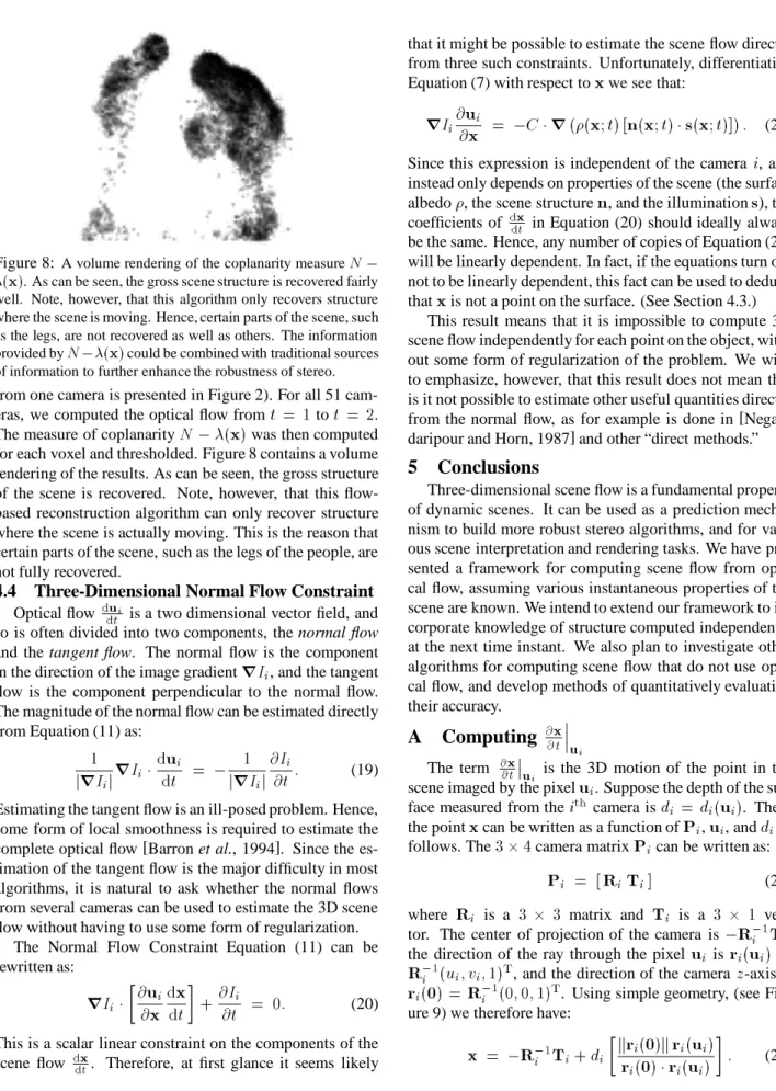
We present the results of this algorithm in Figure 8. We used the data from all 51 cameras of the CMU Virtualized Reality dome [Narayanan et al., 1998] (Some of the data

Figure 8: A volume rendering of the coplanarity measureN,

(x). As can be seen, the gross scene structure is recovered fairly

well. Note, however, that this algorithm only recovers structure where the scene is moving. Hence, certain parts of the scene, such as the legs, are not recovered as well as others. The information

provided byN,(x)could be combined with traditional sources

of information to further enhance the robustness of stereo.

from one camera is presented in Figure 2). For all 51 cam-eras, we computed the optical flow fromt = 1tot = 2.

The measure of coplanarityN ,(

x

)was then computed

for each voxel and thresholded. Figure 8 contains a volume rendering of the results. As can be seen, the gross structure of the scene is recovered. Note, however, that this flow-based reconstruction algorithm can only recover structure where the scene is actually moving. This is the reason that certain parts of the scene, such as the legs of the people, are not fully recovered.

4.4 Three-Dimensional Normal Flow Constraint

Optical flow du i

dt

is a two dimensional vector field, and so is often divided into two components, the normal flow and the tangent flow. The normal flow is the component in the direction of the image gradientrI

i, and the tangent

flow is the component perpendicular to the normal flow. The magnitude of the normal flow can be estimated directly from Equation (11) as:

1 jrI i j rI i d

u

i dt = , 1 jrI i j @I i @t : (19)

Estimating the tangent flow is an ill-posed problem. Hence, some form of local smoothness is required to estimate the complete optical flow [Barron et al., 1994]. Since the es-timation of the tangent flow is the major difficulty in most algorithms, it is natural to ask whether the normal flows from several cameras can be used to estimate the 3D scene flow without having to use some form of regularization.

The Normal Flow Constraint Equation (11) can be rewritten as: rI i @

u

i @

x

d

x

dt + @I i @t = 0: (20)

This is a scalar linear constraint on the components of the scene flow dx

dt

. Therefore, at first glance it seems likely

that it might be possible to estimate the scene flow directly from three such constraints. Unfortunately, differentiating Equation (7) with respect to

x

we see that:

rI i @

u

i @

x

= ,Cr((

x

;t)[

n

(

x

;t)

s

(

x

;t)]): (21)

Since this expression is independent of the camera i, and

instead only depends on properties of the scene (the surface albedo, the scene structure

n

, and the illumination

s

), the

coefficients of dx dt

in Equation (20) should ideally always be the same. Hence, any number of copies of Equation (20) will be linearly dependent. In fact, if the equations turn out not to be linearly dependent, this fact can be used to deduce that

x

is not a point on the surface. (See Section 4.3.)

This result means that it is impossible to compute 3D scene flow independently for each point on the object, with-out some form of regularization of the problem. We wish to emphasize, however, that this result does not mean that is it not possible to estimate other useful quantities directly from the normal flow, as for example is done in [Negah-daripour and Horn, 1987] and other “direct methods.”

5

Conclusions

Three-dimensional scene flow is a fundamental property of dynamic scenes. It can be used as a prediction mecha-nism to build more robust stereo algorithms, and for vari-ous scene interpretation and rendering tasks. We have pre-sented a framework for computing scene flow from opti-cal flow, assuming various instantaneous properties of the scene are known. We intend to extend our framework to in-corporate knowledge of structure computed independently at the next time instant. We also plan to investigate other algorithms for computing scene flow that do not use opti-cal flow, and develop methods of quantitatively evaluating their accuracy.

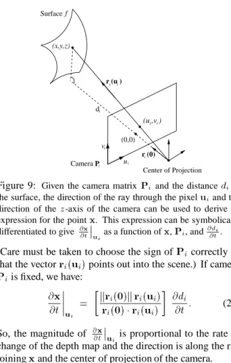
A

Computing

@x @t u i The term @x @t ui

is the 3D motion of the point in the scene imaged by the pixel

u

i. Suppose the depth of the

sur-face measured from thei th camera isd i =d i (

u

i ). Then,

the point

x

can be written as a function of

P

i,

u

i, and d

ias

follows. The34camera matrix

P

ican be written as:

P

i = [

R

i

T

i ] (22) where

R

i is a 3 3 matrix and

T

i is a 3 1

vec-tor. The center of projection of the camera is ,

R

,1

i

T

i,

the direction of the ray through the pixel

u

i is

r

i (

u

i ) =

R

,1 i (u i ;v i ;1) T

, and the direction of the cameraz-axis is

r

i (

0

) =

R

,1 i (0;0;1) T

. Using simple geometry, (see Fig-ure 9) we therefore have:

x

= ,

R

,1 i

T

i +d i k

r

i (

0

)k

r

i (

u

i )

r

i (

0

)

r

i (

u

i ) : (23)

ui vi (u ,v )i i di 0 0 1 1 00 00 11 11 0 1 0 0 1 1 (x,y,z) Camera Pi f Surface (0,0) Center of Projection r (u ) r (0)i i i

Figure 9: Given the camera matrix P

i and the distance

d

i to

the surface, the direction of the ray through the pixeluiand the

direction of the z-axis of the camera can be used to derive an

expression for the pointx. This expression can be symbolically

differentiated to give @x @t ui as a function ofx,P i, and @d i @t :

(Care must be taken to choose the sign of

P

icorrectly so

that the vector

r

i (

u

i

)points out into the scene.) If camera

P

iis fixed, we have: @

x

@t ui = k

r

i (

0

)k

r

i (

u

i )

r

i (

0

)

r

i (

u

i ) @d i @t : (24)

So, the magnitude of @x @t

ui

is proportional to the rate of change of the depth map and the direction is along the ray joining

x

and the center of projection of the camera.

References

[Adelson and Bergen, 1991] E. Adelson and J. Bergen. The plenoptic function and the elements of early vision. In Landy and Movshon, editors, Computational Models

of Visual Processing. MIT Press, 1991.

[Avidan and Shashua, 1998] S. Avidan and A. Shashua. Non-rigid parallax for 3D linear motion. In Proc. of

CVPR ‘99, volume 2, pages 62–66, 1998.

[Barron et al., 1994] J.L. Barron, D.J. Fleet, and S.S. Beauchemin. Performance of optical flow techniques.

IJCV, 12(1):43–77, 1994.

[Collins, 1996] R.T. Collins. A space-sweep approach to true multi-image matching. In Proc. of CVPR ’96, pages 358–363, 1996.

[Costeira and Kanade, 1998] J.P. Costeira and T. Kanade. A multibody factorization method for independently moving objects. IJCV, 29(3):159–179, 1998.

[Horn, 1986] B.K.P. Horn. Robot Vision. McGraw Hill, 1986.

[Liao et al., 1997] W.-H. Liao, S.J. Aggrawal, and J.K. Aggrawal. The reconstruction of dynamic 3D structure of biological objects using stereo microscope images.

Machine Vision and Applications, 9:166–178, 1997.

[Malassiotis and Strintzis, 1997] S. Malassiotis and M.G. Strintzis. Model-based joint motion and structure esti-mation from stereo images. CVIU, 65(1):79–94, 1997. [Metaxas and Terzopoulos, 1993] D. Metaxas and D.

Ter-zopoulos. Shape and nonrigid motion estima-tion through physics-based synthesis. IEEE PAMI,

15(6):580–591, 1993.

[Narayanan et al., 1998] P.J Narayanan, P.W. Rander, and T. Kanade. Constructing virtual worlds using dense stereo. In Proc. of the Sixth ICCV, pages 3–10, 1998. [Negahdaripour and Horn, 1987] S. Negahdaripour and

B.K.P. Horn. Direct passive navigation. PAMI,

9(1):168–176, 1987.

[Penna, 1994] M.A. Penna. The incremental approxima-tion of nonrigid moapproxima-tion. CVGIP, 60(2):141–156, 1994. [Pentland and Horowitz, 1991] A.P. Pentland and

B. Horowitz. Recovery of nonrigid motion and structure. IEEE PAMI, 13(7):730–742, 1991.

[Rander et al., 1996] P.W. Rander, P.J Narayanan, and T. Kanade. Recovery of dynamic scene structure from multiple image sequences. In Proc. of the 1996 Intl.

Conf. on Multisensor Fusion and Integration for Intelli-gent Systems, pages 305–312, 1996.

[Seitz and Dyer, 1997] S.M. Seitz and C.M. Dyer. Photo-realistic scene reconstrcution by space coloring. In Proc.

of CVPR ’97, pages 1067–1073, 1997.

[Shi et al., 1994] Y.Q. Shi, C.Q. Shu, and J.N. Pan. Uni-fied optical flow field approach to motion analysis from a sequence of stereo images. Pattern Recognition,

27(12):1577–1590, 1994.

[Ullman, 1979] S. Ullman. The Interpretation of Visual

Motion. MIT Press, 1979.

[Ullman, 1984] S. Ullman. Maximizing the rigidity: The incremental recovery of 3-D shape and nonrigid motion.

Perception, 13:255–274, 1984.

[Waxman and Duncan, 1986] Allen M. Waxman and James H. Duncan. Binocular image flows: Steps toward stereo-motion fusion. IEEE PAMI, 8(6):715–729, 1986. [Young and Chellappa, 1999] G.S. Young and R. Chel-lappa. 3-D motion estimation using a sequence of noisy stereo images: Models, estimation, and unique-ness. IEEE PAMI, 12(8):735–759, 1999.

[Zhang and Faugeras, 1992a] Z. Zhang and O. Faugeras.

3D Dynamic Scene Analysis. Springer-Verlag, 1992.

[Zhang and Faugeras, 1992b] Z. Zhang and O. Faugeras. Estimation of displacements from two 3-D frames ob-tained from stereo. IEEE PAMI, 14(12):1141–1156,