EXPLORING ISSUES OF BALANCED VERSUS IMBALANCED
SAMPLES IN MAPPING GRASS COMMUNITY IN THE
TELPERION RESERVE USING HIGH RESOLUTION IMAGES
AND SELECTED MACHINE LEARNING ALGORITHMS
By
Isoa, Mary Itohan (1531061)
SUPERVISOR: Dr Elhadi Adam
A dissertation report submitted to the Faculty of Science, University of the
Witwatersrand, Johannesburg, in partial fulfilment of the requirements for the
degree of Master of Science (GIS and Remote Sensing).
MARCH 2018
ABSTRACT
Accurate vegetation mapping is essential for a number of reasons, one of which is for conservation purposes. The main objective of this research was to map different grass communities in the game reserve using RapidEye and Sentinel-2 MSI images and machine learning classifiers [support vector machine (SVM) and Random forest (RF)] to test the impacts of balanced and imbalance training data on the performance and the accuracy of Support Vector Machine and Random forest in mapping the grass communities and test the sensitivities of pixel resolution to balanced and imbalance training data in image classification. The imbalanced and balanced data sets were obtained through field data collection.
The results show RF and SVM are producing a high overall accuracy for Sentinel-2 imagery for both the balanced and imbalanced data set. The RF classifier has yielded an overall accuracy of 79.45% and kappa of 74.38% and an overall accuracy of 76.19% and kappa of 73.21% using imbalanced and balanced training data respectively. The SVM classifier yielded an overall accuracy of 82.54% and kappa of 80.36% and an overall accuracy of 82.21% and a kappa of 78.33% using imbalanced and balanced training data respectively.
For the RapidEye imagery, RF and SVM algorithm produced overall accuracy affected by a balanced data set leading to reduced accuracy. The RF algorithm had an overall accuracy that dropped by 6% (from 63.24% to 57.94%) while the SVM dropped by 7% (from 57.31% to 50.79%). The results thereby show that the imbalanced data set is a better option when looking at the image classification of vegetation species than the balanced data set.
The study recommends the implementation of ways of handling misclassification among the different grass species to improve classification for future research. Further research can be carried out on other types of high resolution multispectral imagery using different advanced algorithms on different training size samples.
iii
DECLARATION
I, Mary Itohan Isoa (1531061), attest that this research is my unassisted work. It is being submitted for the degree of Master of Science at the University of Witwatersrand, Johannesburg. It has not been submitted at any other University for an examination or degree.
Signature: Date: 23rd day of March 2018
iv
Dedication
I dedicate this research to my brother, Thomas, for his support all round
in helping me to achieve this accomplishment. There cannot be enough
thanks to you for your unfailing support and continuous encouragement
throughout my years of study. This could not have been done without
you.
v
Acknowledgments
All praise and honour go to God Almighty for His mercies and favours in my life, especially during this program.
My sincerest gratitude goes to my supervisor Dr. Elhadi Adam for his guidance and support not just throughout my research, but during the master's program. Your support gave me the opportunity to improve my knowledge on remote sensing.
vi TABLE OF CONTENTS Acknowledgments……….……….v LIST OF FIGURES……….………viii LIST OF TABLES……….………...ix LIST OF ABBREVIATIONS……….……..ix 1.1. General Introduction ... 2 1.2. Problem Statement ... 5
1.3. Aims and objectives ... 6
2.1. Mapping grass communities using remote sensing ... 8
2.1.1. Importance and principle of mapping grass communities ... 9
2.2. Mapping grass communities using multispectral remote sensing ... 9
2.3. Mapping grass community using hyperspectral remote sensing ... 10
2.4. Mapping grass communities using new advanced multispectral data ... 11
2.5. Ground and training sampling for mapping grass communities ... 11
2.6. Machine learning classifiers for mapping grass communities ... 12
2.7. Conclusion ... 14
3.1. Study area ... 16
3.2. Remote sensing data acquisition and pre-processing ... 18
3.2.1. Sentinel-2 Multispectral Instrument (MSI) image acquisition ... 18
3.2.2. RapidEye image acquisition ... 19
3.3. Remote sensing data pre-processing ... 20
3.4. Field data collection ... 20
3.5. Image classification ... 22
3.5.1. Support Vector Machines ... 23
3.5.2. Random forest classifiers ... 28
3.6. Accuracy assessment... 30
4.1. Optimization of RF parameters ... 32
4.1.1. Sentinel-2 MSI imagery ... 32
vii
4.2. Parameter tuning of SVM ... 35
4.2.1. Sentinel-2 MSI ... 35
4.2.2. RapidEye imagery ... 35
4.3. RF and SVM performance in mapping grass community ... 35
4.3.1. Sentinel-2 MSI imagery (imbalanced training data) ... 35
4.3.2. Sentinel-2 MSI imagery (balanced training data) ... 36
4.3.3. RapidEye imagery (imbalanced training data) ... 37
4.3.4. RapidEye imagery (balanced training data) ... 38
4.4. RapidEye and Sentinel-2 bands significance ... 39
4.4.1. Sentinel-2 MSI imagery (balanced training data) ... 39
4.4.2. Sentinel-2 MSI imagery (imbalanced training data) ... 40
4.4.3. RapidEye Imagery (balanced training data) ... 42
4.4.4. RapidEye imagery (imbalanced training data) ... 43
4.5. Accuracy assessment... 45
4.5.1. Sentinel-2 MSI (balanced dataset) ... 45
4.5.2. Sentinel-2 MSI (imbalanced dataset) ... 45
4.5.3 RapidEye imagery (balanced dataset) ... 50
4.5.4. RapidEye imagery (imbalanced dataset) ... 50
5.1. Discussion ... 58
5.2. Conclusion ... 59
viii
LIST OF FIGURES
Figure 1: The location of Telperion Nature Reserve………....….17
Figure 2: Support vector machine linear classifier………24
Figure 3: Support vector machine non-linear classifier……….…25
Figure 4: The Main idea of support vector machine………..26
Figure 5: Workflow and main idea of Random forest………...27
Figure 6: RF parameter optimization for imbalanced and balanced data of Sentinel-2………...………..….33
Figure 7: RF parameter optimization for imbalanced and balanced data of RapidEye………34
Figure 8: Vegetation mapping classification using RF and SVM classification algorithm for Sentinel-2 (imbalanced)……….36
Figure 9: Vegetation mapping classification using RF and SVM classification algorithm for Sentinel-2 (balanced)……….37
Figure 10: Vegetation mapping classification based using RF and SVM classification algorithm for RapidEye (imbalanced)……….……...38
Figure 11: Vegetation mapping classification using RF and SVM classification algorithm for RapidEye (imbalanced)………...………...39
Figure 12: Sentinel-2 band significance in vegetation classification for all vegetation species and for each vegetation species (balanced)……...………..……….40
Figure 13: Sentinel-2 band significance in vegetation classification for all vegetation species and for each vegetation species (imbalanced)………...………....41
Figure 14: RapidEye band significance in vegetation classification for all vegetation species and for each vegetation species (balanced)…...………...43
Figure 15: RapidEye band significance in vegetation classification for all vegetation species and for each vegetation species (imbalanced)……...………...…44
ix
LIST OF TABLES
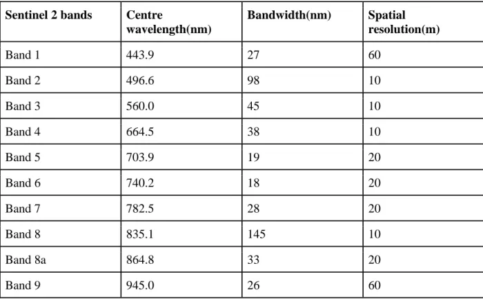
Table 1: Spectral bands of Sentinel 2 A imagery………..………18
Table 2: Spectral bands of RapidEye imagery………...19
Table 3: Training and test data for grass species (Imbalanced)……….21
Table 4: Training and test data for grass species (Balanced)……….22
Table 5: Confusion matrix for Sentinel-2 using Random Forest (Imbalanced)……….46
Table 6: Confusion matrix for Sentinel-2 using Support vector machines (Imbalanced)……….47
Table 7: Confusion matrix for Sentinel-2 using Random Forest (Balanced)………48
Table 8: Confusion matrix for Sentinel-2 using Support vector machines (Balanced)………….49
Table 9: Confusion matrix for RapidEye using Random Forest (Imbalanced)……….52
Table 10: Confusion matrix for RapidEye using Support vector machines (Imbalanced)………53
Table 11: Confusion matrix for RapidEye using Random Forest (Balanced)………...…54
Table 12: Confusion matrix for RapidEye using Support vector machines (Balanced)…………55
Table 13: OA of RF and SVM for RapidEye and Sentinel2 images of both balanced and imbalanced data set………56
LIST OF ABBREVIATIONS
RS= Remote sensing
MSI= Multispectral instrument ESA= European Space Agency SVM= Support Vector machines RF= Random Forest
GPS=Global Positioning System SWIR= Short Wave Infrared
1
CHAPTER ONE
2
1.1. General Introduction
There has been a tremendous need for land cover maps for the observation and sustenance of the earth's natural resources (Foley et al. 2005; Verburg et al. 2011; Hansen 2012). These maps are used in urban planning, land cover assessment and conservation (Wessels et al. 2003; Gebhardt et al. 2014; Fry et al. 2011). Grasslands are one of the world's most famous types of land cover vegetation (Latham et al. 2014). They play an essential role in plant biodiversity (Bergman et al. 2008; van Swaay, 2002) and spatial heterogeneity (MacFayden et al. 2016).
When mapping grass species, field-based methods have been used in the past at a local scale (Ramoelo et al. 2015). The main advantage of using field based methods is that they are useful when mapping vegetation species of a small area. However, studies have shown the field-based method for grass communities mapping is time-consuming, expensive and sometimes some areas were inaccessible leading to insufficient data (Ling et al. 2014; Kavzoglu and Colkesen, 2009a; Ramoelo et al. 2013). Remote sensing has proven to be a preferred and useful method in mapping vegetation because of its ability in discerning and observing the physical features of an area by assessing its reflected and emitted radiation at an extent from the targeted area (Mutanga, Adam and Cho, 2012). Satellite images help scientists and researchers to understand the earth better as these images allow them to see much more than they would if they were observing the surface from the ground. Remote sensing data offers a more precise alternative to field survey data, especially when dealing with cost and effectiveness. Remote sensing has shown to be very helpful in land cover mapping (Tucker et al. 1985), crop monitoring (Wu et al. 2015) and climate studies (Yang et al. 2013). This rise in interest is predominantly due to the current revolution in data, technologies and conjecture in urban remote sensing (Weng and Quattrochi, 2007; Yang et al. 2013; Salehi et al. 2012).
Multispectral remote sensing (Akasheh et al. 2008; Saatchi et al. 2007) and hyperspectral data (Lawrence et al. 2006; Peerbhay et al. 2013) have both been used in vegetation mapping. Multispectral data, such as SPOT and Landsat TM imagery are limited by their spatial and spectral resolution, which is ineffective in proper vegetation mapping because of its broad bands (Govender et al. 2008). Hyperspectral imagery, on the other hand, has narrow spectral bands
3
which makes it a more efficient method in mapping vegetation and in land cover use (Koch et al. 2005) as it can identify surface features at a higher spectral resolution. Hyperspectral data come with the challenge of data processing and analysis due to high dimensionality which can lead to inadequate classification and performance of the classification algorithm (Tsai et al. 2007; Kavzoglu and Mather, 2002). The arrival of some new generation sensors such as the Worldview 2 and 3, Sentinel 2 MSI as well as RapidEye have been used more recently for mapping grass communities and vegetation species in a more extensive area (Huang et al. 2017; Sibanda et al. 2017; Drusch et al. 2012).
Classification of remotely sensed images continues to be a difficult task. The set size of the training sample, the spatial resolution of the image, the diversity of vegetation class, attribute of the classification algorithm are some of the factors that have a considerable effect on the classification accuracy (Lu and Weng, 2007; Kavzoglu, 2009). Image classification has proven to be quite essential in remote sensing application. Hence, the importance of using advanced algorithm classifiers. A wrongly classified image can lead to information that is worthless and inadequate. It could also have an unfavourable effect if decisions are based on incorrect classification. Let us say, for example, that image classification was carried out on a satellite image where the grass was incorrectly classified as water. Such a mistake would prove detrimental in urban development or water management. Therefore, image classification plays a vital role in mapping and image interpretation (Li et al. 2014; Ma et al. 2017). Machine learning algorithms are productive and effective because they are not dependent on data scattering assumptions (e.g., Normality) and have positive accuracy (Foody, 1995a; Friedl and Brodley, 1997).
The design of the training samples is of importance. The training sets in many instances determine the quality of supervised classification (Smola and Scholkopf, 2003). In reality, though, classifiers are highly imbalanced or occur in unknown proportions. The spectral characteristics of remote sensing data provide a lot of distinguishing and decisive factors such as near-infrared band or vegetation indices for the plants, forestry and agricultural utilization (Kim and Yeom, 2015). Traditional learning methods are intended principally for balanced samples. A balanced sample has uniformity of classes across the class distribution. When algorithms are
4
used for imbalanced samples, there tends to be over predicting the appearance of the majority class (Wei and Dunbrack, 2013). A balanced sample is believed to boost overall classification in contrast to an imbalanced sample (He, 2011; Laurikkala, 2001). The characteristics and quality of the training samples are essential in classification which directly impacts classification accuracy (Foody, 1999; Ustuner et al. 2016). Errors, such as interpretation problems and poor quality of training data sets can affect accuracy. The set size of a training sample is essential when classifying minor classes of interest (Ustuner et al. 2016). In some cases, the training sample of one class could differ from another class. This is known as imbalanced training samples. This imbalance leads to low accuracy for minor classes (Foody et al. 2006).
Image classification methods, using remotely sensed data is generally used when mapping grass species. The option of the suitable remotely sensed data in terms of the price and the resolutions and the choice of suitable classification process are critical for valid, accurate vegetation mapping (Adam et al. 2014). There are various types of machine learning algorithm, and the model used is dependent on the user's familiarity with the algorithm and what the user wants to achieve. When it comes to vegetation mapping and remote sensing in general, the two most commonly used are the support vector machine (SVM) and random forest (RF) (Clark et al. 2016; Mountrakis et al. 2011). SVM is a simplified algorithm used when dealing with imbalanced dataset because it handles high dimensionality which is a problem when processing small training samples and the need to achieve high accuracy (Melgani and Bruzzone, 2004; Foody et al. 2006). SVM is greatly reliant on the training sample size (Schohn and Cohn, 2000). Random forest (RF) involves re-sampling the original training samples to increase accuracy and stability. Rodriguez-Galiano et al. (2012), and Pal (2005) is of the opinion that random forest is more robust when it comes to variation in data. Studies have shown that a balanced sample improves overall classification in cases like SVM and RF in comparison to the imbalanced sample (Estabrooks et al. 2004; Weiss and Provost, 2003).
This study looks at the effects, if any, of a balanced and imbalanced dataset on high-resolution images, RapidEye and Sentinel 2, using SVM and RF classifier.
5
1.2. Problem Statement
Field-based methods are commonly being used to collect data on varying grass species in the Telperion Game Reserve. This is a tedious and time-consuming method that can lead to inaccuracy in classifying the various grass communities, as access to some areas might be a problem. For proper management of the reserve, reliable, current and comprehensive spatial information on the biodiversity of the area is essential (Adam et al. 2010). Remote sensing provides vital information on grass community and its distribution (Darvishzadeh et al. 2008). High-resolution imagery like Sentinel 2 and RapidEye are preferred in research in land cover and vegetation mapping due to global coverage and free access. It is not just the image selected that is important, but also the classification method used as this affects the results of the land cover maps (Lu and Weng, 2007). Of the machine learning-based algorithms, RF and SVM are becoming popular in image classification research (Adam et al. 2014) primarily due to their insensitivity to overtraining and noise, making them better suited to deal with imbalanced data (Breiman, 2001). The design and selection of training samples are significant in the learning stage of a classifier (Ustuner et al. 2016). It is always best to use a balanced sample when dealing with machine learning algorithms (Weiss and Provost, 2003; Japkowicz and Stephen, 2002). Most times the method used to balance the samples depends on the researcher and what they are trying to achieve (Chawla et al. 2002; Chen et al. 2004; Trebar and Steele, 2008). It is believed that a substantial quantity of training samples is vital for image classification and is collected as ground truth data from the field (Hubert-Moy et al. 2002; Mather, 2004). When dealing with high resolution images, a good number of samples are needed because of high sample variation (Tsai et al. 2007; Borges et al. 2007). There is the need to find the optimum number of samples needed for higher spatial resolutions regarding the number of samples and balanced and imbalanced samples across different satellite images and classification algorithm. In the past, studies have tested imbalanced and balanced training sample in individual machine learning classifiers such as RF and SVM (Mellor et al. 2014; Ustuner et al. 2016). Only a finite amount of research has been carried out to compare different classifiers in different high-resolution images using both balanced and imbalanced datasets and its effect if any on the overall accuracy.
6
1.3. Aims and objectives
This research aims to investigate the impacts of balanced and imbalanced samples on the accuracy of grass community mapping using different machine learning classifiers, and high resolution multispectral remotely sensed data.
The specific objectives are to,
● Map different grass communities in the Telperion Game Reserve using RapidEye and Sentinel 2 images and machine learning classifiers (Support vector machine and Random forest).
● To quantify and analyse the impacts of balanced and imbalanced training data on the performance and the accuracy of Support Vector Machine and Random forest in mapping the grass communities.
● To test the sensitivities of pixel resolution to balanced and imbalance training data in image classification.
7
CHAPTER TWO
8
2.1. Mapping grass communities using remote sensing
Vegetation mapping analysis has become predominant in recent years (Cingolani et al. 2004) because they help in differentiating grass species and ecology in an area which leads to valuable information in conservation management (Zhang et al. 2016) and management practices. The traditional field method technique of mapping vegetation is a tedious task used in gaining knowledge about species type and their makeup (Terri and Stowe 1976). This method needs intensive fieldwork and laboratory analysis to measure the biochemical and biophysical properties of the grass species (Mutanga et al. 2003). The intense nature of fieldwork leads to results that are not fully representative of plant population and its distribution, especially in areas of varied diversity (Mutanga et al. 2003). The use of field data alone is insufficient as current and accurate information is required in a proper land cover and vegetation mapping, especially for areas of diverse landscapes (Odindi et al. 2016).
Remote sensing provides an alternative and economical way of analysing grass species as it reduces the field work and the laboratory analysis required by the traditional method. The use of remote sensing has helped in providing information of even the most inaccessible areas at a cost-effective rate (Running et al. 1993; Darvishzadeh et al. 2008). Remotely sensed data has been used in discriminating grassland species (Baldi et al. 2006; Toivonen and Luoto, 2003; Wang et al. 2010). Recent studies in mapping and monitoring vegetation species have incorporated the use of low and medium resolution imagery such as Landsat (Wulder et al. 2008; Vogelman et al. 1998; Giri et al. 2003), SPOT (Kanellopoulos et al. 1992; Chen, Franklin and Spies, 1992) and MODIS (Stefanov and Netzband 2005). The accuracy of using these types of imagery is compromised by their spectral and spatial resolution (Foody 2002). The introduction of multispectral and hyperspectral imaging has dramatically improved the accuracy of vegetation mapping worldwide as they have high spectral and spatial resolution (Mutanga, Adam and Cho, 2012; Akasheh et al. 2008; Harvey and Hill, 2001; Lawrence et al. 2006). New generation imagery such as Worldview 2&3, Sentinel 2 MSI, and RapidEye has emerged recently. Their spectral bands which fall in the electromagnetic spectrum, such as red edge provides a more detailed classification of landscapes (Schuster et al. 2012; Cho et al. 2012; Mutanga, Adam and Cho, 2012). While these new multispectral sensors advantageously provide significant details in
9
mapping vegetation (Baumstark et al. 2016; Odindi et al. 2014; Omer et al. 2015), acquiring the data is expensive. Image analysis, through the use of vegetation indices, is a standard way in remote sensing for discerning spatial patterns of the distribution of vegetation (Adjorlolo et al. 2012). Remote sensing can also be used to distinguish between local grassland communities, grasslands and frequently co-occurring vegetation species. This is done by comparing classification results from different imagery dataset (Melville et al. 2018). The selection of the appropriate sensor is vital for vegetation mapping and land cover. Low-resolution images are commonly used in the large scale mapping of the identification of a substantial number of vegetation classes while a higher resolution image is used for superior classification of vegetation at a smaller scale. High-quality ground truth data is needed in remote sensing for cross-validation and training algorithm. To this effect, remote sensing is a potent tool when used concurrently with ground truth data (Bredenkamp et al. 1998).
2.1.1. Importance and principle of mapping grass communities
Monitoring land cover is essential for global change investigation (Jung et al. 2006; Lambin et al. 2001). Proper mapping of grass and vegetation species is crucial in managing the earth's natural resources as vegetation supplies a foundation for all living beings (Xiao et al. 2004). Vegetation mapping also includes details about natural and human-made habitat by quantifying vegetation cover at a small or large scale either presently or over an extended period of time (Xie et al. 2008). For proper conservation, it is crucial to obtain new generation cover (Egbert et al. 2002; He et al. 2005). The principle of vegetation mapping using remote sensing, relies on the spectral attribute of the vegetation species and their spectral reflectance and radiance.
2.2. Mapping grass communities using multispectral remote sensing
Multispectral data have been used in vegetation mapping on many occasions (Rignot et al. 1997; Harvey and Hill 2001; Chastain, et al. 2008; Martinez-Lopez et al. 2014). In multispectral imagery, the pixels lead to a mix of vegetation species in varying proportion (Zomer et al. 2009). This mixing is primarily because multispectral sensors give rise to three to six spectral bands spanning from visible to near-infrared of the electromagnetic spectrum (Jensen, 2007). This mixing effect is a significant disadvantage in mapping vegetation. Mansour et al. (2016) used
10
multispectral remote sensing for mapping grassland degradation. Huang and Siegert (2006) found that SPOT VGT imagery was useful in detecting environmental changes on a larger scale and SPOT images were used to produce vegetation maps in Eastern New Zealand (Mathieu et al. 2006). Zheng et al. (2006) used Landsat TM images to analyse wetland landscape patterns on the Minjiang River. Landsat images are one of the more common types of low to medium resolution images used. Wang et al. (2007) used Quickbird-2 to map aquatic and terrestrial vegetation. Multispectral data were also used for global mapping at a continental scale to map land cover in Central Africa using AVHRR (Mayaux et al. 1998).
Although mapping vegetation using multispectral remote sensing has been promising, there are limitations due to its lower spatial and spectral resolutions, especially when dealing with complex and diverse vegetation types (Adam et al. 2012; Feng et al. 2015).
2.3. Mapping grass community using hyperspectral remote sensing
Hyperspectral remotely sensed data records a large quantity of narrow wavelength bands (over 200) from the visible, near infrared, mid-infrared to the shortwave infrared bands of the electromagnetic spectrum. These bands offer new vegetation index for specific species (Clevers et al. 2007) making it more efficient in vegetation mapping. An advantage of this type of imagery is that the mixed pixel problem seen in multispectral imaging is significantly reduced, providing more information on land cover (Lu and Weng, 2009). Mutanga and Skidmore (2004) using hyperspectral data deduced that the narrowband indices provided better information on grassland biomass. Some researchers have focused on vegetation density (Nichol and Lee, 2005; Small, 2003) while others focused on the creation of land use/land cover maps (Carleer and Wolff 2006; Herold et al. 2003). Vegetation species classified as Invasive species have been successfully mapped using hyperspectral imagery because of its ability in determining the percentage coverage of vegetation species (Mundt al. 2005; Williams and Hunt, 2004; Glenn et al. 2005; Lawrence et al. 2006)
A disadvantage of this though is the problem caused by shadows (Asner and Warner, 2003; Zhou et al. 2008; Lu and Weng, 2009). These shadows can lead to lower accuracy if a suitable
11
classification algorithm and image processing method is not used (Irons et al. 1985; Cushnie, 1987). This problem was examined recently (Zhou et al. 2008; Mathieu et al. 2007; Walter, 2004; Zhang et al. 2003). High spectral variation is also a problem when dealing with similar land cover types. Object-oriented classification methods have reduced this problem significantly (Mathieu et al. 20007; Zhou et al. 2008; Stow et al. 2007; Jacquin et al. 2008; Laliberte et al. 2004). Another setback of hyperspectral data is that they are expensive (Sibanda et al. 2017).
2.4. Mapping grass communities using new advanced multispectral data
The arrival of new multispectral sensors has been recognized as an improvement from the shortfalls of hyperspectral and multispectral imagery (Mutanga et al. 2012). The higher spatial resolution and extended amount of bands such as the red edge, are preferred for vegetation mapping at higher accuracies (Mansour and Mutanga, 2012; Adelabu, Mutanga and Adam, 2015). RapidEye and WorldView-2&3 imagery is used in various vegetation mapping research (Ustuner et al. 2016; Adam et al. 2014; Luck-Vogel et al. 2016; Adam et al. 2017). Mansour and Mutanga (2012) used WorldView-2 data to map grassland degradation of grass species in South Africa with an overall accuracy of 90%. The addition of a red-edge band helps in discerning variations in vegetation which makes for improved vegetation mapping. Despite these many advantages, these images are expensive. The availability of Sentinel-2 MSI, which also has high spatial and spectral properties, has helped in this aspect as it can be acquired free of charge.
High spectral resolution does not often translate to improved accuracy; thus more advanced and robust classifiers are required (Sesnie et al. 2010; Adelabu et al. 2015; Lawrence et al. 2006). These include classifiers such as SVM and RF.
2.5. Ground and training sampling for mapping grass communities
While remotely sensed data is vital for proper vegetation mapping, ground truth data are equally essential for cross-validation when dealing with remote sensing data (Odindi et al. 2016; Bredenkamp et al. 1998). If the number of samples from the field is not enough, sometimes points are digitized based on proper georeferencing. Sometimes, vectors are manually digitized
12
(Evans et al. 2012; Al-Mashreki et al. 2010). Millard and Richardson (2015) suggested that the training and testing data should be as numerous as possible.
Hubert-Moy et al. (2001) and Mather, (2004) believed that an adequate amount of training samples is vital for the classification of images and are collected as ground truth data from the field. The training data size is thought to affect the accuracy of classification performance (Mellor et al. 2015; Millard and Richardson, 2015). A substantial amount of training and testing data is believed to be needed to assess the classification accuracy entirely (Jin et al. 2014). Sometimes, the distribution of test sample may be different from that of the training sample, and the actual effects of this miscalculation might not be realized at the learning stage. In recent years, studies have shown the importance of a balanced sample over an imbalanced sample (Japkowicz and Stephen, 2002; Wei and Dunbrack, 2003; Estabrooks et al., 2004; Weiss and Provost, 2003). In a real-world scenario, imbalanced training samples occur due to difficulty obtaining the ground sample for some areas. Mellor (2017) showed that deliberately imbalancing a dataset can improve classification and performance of some classes without undermining overall classification outcome.
Some studies have shown that using an imbalanced sample can lead to low classification accuracy (Kubat and Matwin, 1997; Japkowicz, 2000). Huang et al., (2002) believed that the training data used, affects the classification accuracy more than the classification algorithm used and suggested an increase in the training sample size to improve classification accuracy.
2.6. Machine learning classifiers for mapping grass communities
Machine learning algorithms are a more accurate type of classification algorithm when dealing with extensive data (Muchoney and Williamson, 2001; Kasischke et al. 2004). They can deal with noisy and missing data, especially classification trees (Simand et al. 2000; Hastie et al. 2001). Different researchers in the past few years have compared various classification algorithms in vegetation mapping. These include maximum likelihood (Stuart et al. 2006) decision trees (Wang et al. 2016), random forest (Vanselow and Samimi, 2014), support vector machines (Schwieder et al. 2016) to neural networks (Zhang and Xie, 2012). Most recently
13
support vector machines and the random forest has been the most commonly used of the classifiers.
Adam et al. (2016) and Pal, (2015) agreed that SVM and RF performed equally well based on high overall accuracy while others showed SVM performed well with a balanced and imbalanced dataset. Ustuner, Sanli and Abdikan (2016) looked at the mapping of diverse vegetation in Aydin, Turkey by classifying a RapidEye imagery using balanced and imbalanced training sample. They used SVM, Maximum Likelihood (ML) and Artificial Neural Network (ANN) classifications for mapping the crop pattern in the area and concluded that SVM was unaffected, showing SVM is an efficient and consistent classifier irrespective of whether it is a balanced or imbalanced training sample. In this case, it is proven that Support vector machine will be a capable and useful classifier. The result further highlighted why the design and choice of training sample into the learning stage of supervised classifiers is so important which is an integral part of this research.
While different algorithms have been used to solve the problem of an imbalanced data sample, random forest and support vector machine have been the most effective. Other methods like weighting and undersampling have been used in the classification of an imbalanced data sample. One such study was that of Anand et al. (2010), who looked at the classification of an imbalanced sample using weighting and undersampling.
There have been a few studies that have been carried out on balanced and imbalanced data samples and the effects of this imbalanced sample set on the overall accuracy and result, but not many have compared this with different high-resolution imagery, hence the focus of this study. The study will look at balanced and imbalanced samples from Sentinel-2 and RapidEye imagery using different algorithms, SVM and RF to determine the factors that affect these sample and if the imaging affects the accuracy of the samples.
14
2.7. Conclusion
Vegetation mapping of diverse grass community class has been done successfully in prior years using different remote sensing imagery both on a local and global scale. A variety of low-medium-high resolution imagery has been used in the past (Mutanga et al. 2016). The new generation multispectral imagery with higher spectral and spatial resolution are being preferred when it comes to mapping vegetation because they possess the red edge band which best classifies these different species. Classification algorithms such as maximum likelihood, k-means, and minimum distance have been used in the past for classification, but the introduction of newer algorithms such as ANN, SVM, and RF is being used more frequently in the present. Only a few researchers have used these advanced classification algorithms on the new generation multispectral imagery using different (balanced and imbalanced) data set.
15
CHAPTER THREE
16
3.1. Study area
The study area is Telperion Nature Reserve (25° 41′ S, 28° 56′ E) depicted in Figure 1 below. The area is approximately 11 000 hectares. Telperion is a section of the more magnificent eZemvelo Nature Reserve, located in Mpumalanga Province of South Africa. The reserve is situated at the border between Gauteng and Mpumalanga Provinces. The Wilge River, which is a tributary of the Oliphant’s River, flows northwards through the reserve. The reserve was established in 2008 and is surrounded by farmlands with people practicing agriculture, specifically maize and sunflower, and cattle rearing. Temperatures range from 140C and 260C during summer and 40C and 170C during winter. Dry winters are experienced here, which makes it difficult for tree growth and ultimately to the death of grassland. There is a high diversity of flowering plants and grass species. Telperion reserve is characterized by highlands and undulating terrain of ridges and valleys. Only 2% of Telperion are officially under conservation. There is a high diversity of animal and birdlife. The Oppenheimer family has owned Telperion for over 40 years.
Mucina and Rutherford (2006) classified the vegetation type as the Bankenveld and Mixed Bushveld. The dominant grass species identified in the sampled plot are Eragrostis gummiflua, Hyparrhenia hirta, Cynodon dactylon, mixed grassland, Eragrostis chloromelas, woody vegetation, wetland grass, Aristida congesta and the Alien Invasive Species.
17
18
3.2. Remote sensing data acquisition and pre-processing
3.2.1. Sentinel-2 Multispectral Instrument (MSI) image acquisition
The Sentinel-2 MSI of the study area was downloaded from the European Space Agency’s website (earthexplorer.usgs.gov) on the 20th of May 2016. Sentinel-2 is a high-resolution multispectral image that was first launched on 23 June 2015. It consists of two similar satellites, Sentinel 2A and Sentinel 2B which helps in frequent revisit every five days under the same viewing angle. Although there can be overlap and some regions will be observed more than once every five days with differing views. It has a spatial resolution of 60m, 20m, and 10m. It consists of thirteen spectral bands with four bands of 10m, six bands of 20m and three bands of 60m (Table 1). It has a 290 kilometre (km) field of view. It was launched to observe natural disaster management, land cover change detection and for other monitoring on the earth’s surface.
Table 1. Spectral bands of Sentinel 2A satellite imagery
Sentinel 2 bands Centre
wavelength(nm) Bandwidth(nm) Spatial resolution(m) Band 1 443.9 27 60 Band 2 496.6 98 10 Band 3 560.0 45 10 Band 4 664.5 38 10 Band 5 703.9 19 20 Band 6 740.2 18 20 Band 7 782.5 28 20 Band 8 835.1 145 10 Band 8a 864.8 33 20 Band 9 945.0 26 60
19
Band 10 1373.5 75 60
Band 11 1613.7 143 20
Band 12 2202.4 242 20
3.2.2. RapidEye image acquisition
A RapidEye imagery map was downloaded from the RapidEye satellite constellation website (rapideye.net/upload) on 21st of May 2016. RapidEye is a high-resolution imagery with multispectral capabilities. It was launched on 29 August 2008 and provides broad area coverage and frequent revisit intervals. RapidEye collects 4 million square kilometres of data per day at 6.5 m ground resolution that can be re-sampled to 5m pixel size. It consists of five satellites equipped with identical sensors located in the same orbital plane. It is capable of daily revisits when off-nadir and revisiting every 5.5days at nadir with a swath width of 77 kilometres (km). It can be used in various fields, including mining, oil and gas exploration, security and emergency, mapping and agriculture. RapidEye imagery is in high demand for land use/land cover maps and mapping vegetation due to its red edge and NIR bands which are sensitive to the chlorophyll content in vegetation. The RapidEye sensors produce imagery in five spectral bands that can be seen in table 2.
Table 2: Spectral bands of RapidEye imagery
Spectral bands Wavelength(nm)
Blue 440-510 Green 520-590 Red 630-685 Red edge 690-730 NIR 760-850
20
3.3. Remote sensing data pre-processing
Georeferencing is extremely important because of the use of different images with different types of the classification algorithm. For the Sentinel-2 MSI image, this was done by selecting the UTM zone 35S with the 10m spatial resolution used. Atmospheric correction was done on both images using the Sen2cor tool which is available in the Sentinel Application Platform (SNAP) toolbox and performed using a python script. The corrected image was then converted to ENVI format, resulting in 10 bands (2-8, 8a, 11 and 12). The converted bands were displayed on ENVI 5.3. Thereafter, the spectral reflectance from the Sentinel 2 MSI image that corresponds to each GPS sampled point was derived.
For the RapidEye imagery, georeferencing was done by selecting UTM zone 35S with a spatial resolution of 5m. The digitized image was in level 3A (orthoproduct) in which radiometric, sensor and geometric corrections have been implemented for the data. The corrected image was displayed on ENVI 5.3. After this was done, the spectral reflectance from the RapidEye image that corresponds to each GPS sampled point was extracted for further analysis. The image was also used in R studio.
3.4. Field data collection
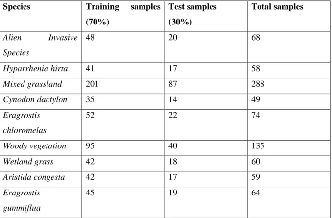
Field data collection was done to locate the different vegetation species in the game reserve. The field sampling was carried out between the 22nd -24th of May 2016, which was consistent with the window period the images were acquired. The sample plots were randomly fixed and spread evenly across the study area (Ramoelo et al., 2012) with the plots being 10 metres x 10 metres in size to account for the pixel size of the sentinel image (10m). It was the dry season at the time the sample was collected. Global Positioning System (GPS) was used to record the coordinates where each of the samples was obtained and also the coordinate of each sample plot with a total of 80 GPS points recorded. The sample collected from each imagery was split into training and testing data using the typical 70:30 split in R studio and ENVI 5.3 respectively for classification. A look at the samples collected shows that they are imbalanced.
21
Table 3: Training and test data for the grass species (imbalanced).
Species Training samples
(70%) Test samples (30%) Total samples Alien Invasive Species 48 20 68 Hyparrhenia hirta 41 17 58 Mixed grassland 201 87 288 Cynodon dactylon 35 14 49 Eragrostis chloromelas 52 22 74 Woody vegetation 95 40 135 Wetland grass 42 18 60 Aristida congesta 42 17 59 Eragrostis gummiflua 45 19 64
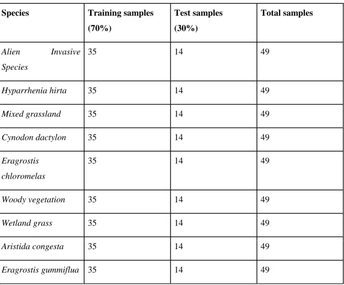
To balance out the imbalanced dataset, a random undersampling method was carried out to even the distribution by randomly reducing the quantity of majority samples while keeping the total of the lowest minority sample in mind and building a more balanced number of samples from that. The balanced data can be seen in table 4 below.
22
Table 4: Training and test data for the grass species (balanced).
Species Training samples
(70%) Test samples (30%) Total samples Alien Invasive Species 35 14 49 Hyparrhenia hirta 35 14 49 Mixed grassland 35 14 49 Cynodon dactylon 35 14 49 Eragrostis chloromelas 35 14 49 Woody vegetation 35 14 49 Wetland grass 35 14 49 Aristida congesta 35 14 49 Eragrostis gummiflua 35 14 49
3.5. Image classification
When it comes to remote sensing, the production of land use and land cover maps is an essential function carried out through image classification (Al-doski et al., 2013). Machine learning algorithms such as SVM and ANN has been tested and examined numerous times in remote sensing, from optical to radar data, for image classification in the current years (Pal et al., 2013). Several studies have shown the superiority of SVM and RF in comparison to other types of classification when dealing with remote sensing images and land cover analysis (Adam et al., 2014; Khatami et al., 2016; Qian et al., 2015; Shao and Lunette, 2012). The frequent use of
23
these two algorithms is why this research focuses on support vector machine and random forest classification algorithms.
3.5.1. Support Vector Machines
Support vector machine is a type of supervised machine learning algorithm that is used for both classification and regression analysis. The concept of SVM is that it creates differing hyperplanes that separate the dataset into a predefined number of classes. The separation is done by using a training sample which is a subset of the dataset. Support vector machines are a powerful kernel-based classification algorithm. Kernel function needs user-defined parameters. Vladimir N. Vapnik invented the original SVM algorithm in 1963. It has since become very popular and has been successful in remote sensing classification. The main reason for SVM's popularity is its high classification accuracy with a small quantity of training data and outperforms other conventional methods like maximum likelihood (Huang et al., 2002). Mountrakis et al. (2011) analysed articles from over a hundred sources and did an overview of the results using SVM as the selected choice of classification and concluded of its high accuracy when dealing with a small training sample and its superiority compared to the other types of classification but its limitations in parameter selection. Camps-Valls et al. (2004) reported SVM's advantage when dealing with hyperspectral remotely sensed data. Although in theory SVM is known for high classification accuracy, it is not as effective when using a significant data because its training difficulty relies heavily on the size of the dataset.
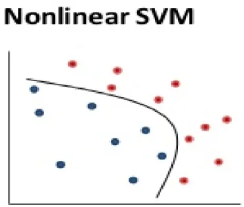
SVM can perform linear classification as well as nonlinear classification, also known as the kernel function. The kernel function transforms the data and then finds the optimal boundary for the outputs. A linear classifier separates points into one of two classes by a straight line, the goal of which is to see a line that passes as far as possible from all aspects to avoid noise (figure 2).
24
Figure 2: linear classifier (source: Vapnik, 1999 Springer; Scholkopf et al., 2002)
Although in real life, most classification tasks are never really this simple as optimal separation would require a more complex structure than that of a straight line as can be seen in the image below. This type of classifier is known as the nonlinear classifier. Hyperplane classifiers are lines drawn to distinguish and separate objects of a different class. This separation is where SVM thrives. SVM is represented by the formula below:
wTx + b = 0
Where w is a weight vector x is input vector
b is bias
The formula also allows us to write the parallel hyperplane (Burgess, 1998)
25
wTx + b < 0 for di = -1 (minus plane)
Where d is the margin of separation (separation between hyperplane and the closest data point for a given w, weight vector and b, bias parameter.
In the figure 3 below, a curve like a backward c, would have to be created to separate the two classes properly.
Figure 3: Nonlinear classifier (source: Vapnik, 1999 Springer; Scholkopf et al., 2002)
Figure 4 represents a nonlinear surface where the data would have to be mapped in a higher dimensional feature space through the kernel function, making them linearly separable in this space since there is no possibility to do so in the original area. When it comes to SVM, the most common kernels are linear, Gaussian radial basis function (RBF), polynomial, and sigmoid kennels which were presented by Fletcher (2009) and Haykin (1999). In remote sensing data analysis, the RBF kernel is the most widely used kernel functions due to its high performance (Gomez-Chova et al., 2011).
26
Where χ is a sample in the data space
χί is a corresponding sample in the feature space γ is the kernel parameter
Figure 4: The Main idea of SVM (source: Statnikov et al., 2011)
A disadvantage of SVM is that it will classify all examples as the majority class, a tactic that if the imbalance is severe, can provide the minimal error rate across the data space (Batuwita, R. and Palade, V., 2012). There have been many works of literature that apply different techniques to the SVM framework to overcome problems due to imbalance (Wu and Chang, 2003). There are various ways of mapping non-linear boundary with kernel functions in SVM which includes linear, polynomial, radial basis function and sigmoid kernels. SVM was run using the support
27
vector classification tool in ENVI 5.3 applying radial basis function (RBF) kernel which is the most commonly used kernel function when dealing with SVM (Pal, Mather 2005; Melgani, Bruzzone 2004; Hermes et al. 1999). The RBF has two tuning parameters- cost (C) and gamma (γ), which can affect overall accuracy (Burges, 1998). The ENVI 5.3 software uses the pairwise classification strategy for multiclass classification. The software carries out classification by selecting the highest probability and a threshold is set, with pixels below this threshold deemed unclassified. Support vector is the interval measured between the nearest points of the two classes (Pal and Mather, 2005). The regions of interest (ROIs) were created by overlaying the dataset on the Sentinel 2 and RapidEye images in ENVI. Once the ROIs were generated, the SVM classification began, after which the training dataset (70%) was used for accuracy assessment. SVM was run for both balanced and imbalanced datasets of RapidEye and Sentinel 2 images. SVM was also run on R using a python script to get the parameter tuning and check the results.
28
3.5.2. Random forest classifiers
Random Forest, developed by Breiman (2001), is a type of supervised classification algorithm. Random forest is based on tree classifiers. In this classifier, the number of decision trees makes the forest. Figure 5 below shows the main idea behind random forest classifiers.
Figure 5: Workflow and main idea of RF (source: Guo et al., 2011)
The random forest classifier uses a set of classification and regression tree, CARTs, to make a prediction (Breiman, 2001). The trees are created through a process known as bagging. Bagging is a method whereby trees are formed by drawing a subset of training samples through replacement. Two-thirds of the samples (referred to as in-bag samples) are used to train the trees while the one third that is left over (referred to as out-of-the-bag samples, OOB) is used for internal cross-validation which helps us estimate how well the RF model performs (Breiman, 2001). There is no pruning when decision trees are produced. The final classification output is created based on a majority vote of the predictions from all individually trained trees (Jin, 2012). The more the trees in the forest, the better the random forest classifier will be. The higher the number of decision trees, the higher the accuracy of the classifier. The decision tree algorithm comes up with a set of rules based on the training data sets. This set of rules is also used on the
29
testing datasets. Random Forest can be used when handling classification and regression issues. Itoperates by constructing a high number of decision trees at the time of training and producing the class that is the mode of the classes (classification) or average prediction (regression) of the individual trees. For RF to be implemented, the user-defined number of trees (ntree) and the user-defined number of features (mtry) must first be set up. The algorithm then creates trees that have a high variance of low bias (Breiman, 2001). The mean average from the trees gives us the predictions of the random forest classification. The RF prediction is described by the formula below
Random forest prediction s = 1
𝑘∑ k
k k−1 th
Where the index k runs over the individual trees in the forest
Random decision forests correct for the decision trees' habit of overfitting to their training set. It is known for being efficient in its implementation on large datasets and its accuracy among current algorithms. It works well with missing data by replacing missing values. This is done by computing the median of all values in the class. It then uses these average values to substitute all the missing values with rough estimates or by doing a raw filling of the missing values by computing proximity. Its accuracy is not affected by this. This approach provides a way of estimating the importance of the individual variables in classification.
One thing about the RF algorithm is that there are a few assumptions involved which lead to faster results and outputs. These assumptions are based on RF creating many decision trees which help in improving the accuracy. RF can rank variables based on the importance of running the mean decrease accuracy table if the user needs further analysis. As earlier stated, the number of trees (ntree) and the number of features in each split (mtry) first have to be set up before RF can be carried out. This optimization was carried out four times- one for each imbalanced RapidEye and Sentinel 2 images and one for each balanced RapidEye and Sentinel 2 images. RF was done in RStudio using a python script. RStudio is an open source tool that supports different geospatial analysis of remotely sensed data. Each run produced different mtry and ntree values.
30
3.6. Accuracy assessment
When it comes to accuracy of classification performance, overall accuracy and kappa coefficient are the most common. Overall accuracy (OA) is the ratio of the number of correctly classified samples (sum of principal diagonal) and the total number of sample units (Congalton and Green, 2009). Accuracy assessment which is an integral part of any classification will be carried out using 30% of the subset of the referenced data. The assessment was done for both images and the balanced and imbalanced dataset. A confusion matrix was also generated which shows predicted class versus actual class. In other words, it shines a light on the errors made by the classifier. Since the research is not based on looking individually at each grass community species, the OA will be used for comparison.
31
CHAPTER FOUR
32
4.1. Optimization of RF parameters
4.1.1. Sentinel-2 MSI imagery
As previously stated, the ntree and mtry can affect the performance of a RF classifier. The ntree and mtry values are represented in grids. For the imbalanced dataset, the mtry value of 4 and ntree value of 2000 created the least OBB error rate of 0.1528962. The highest OBB error rate of 0.177707 was produced by the mtry value of 7 and ntree value of 3000 (Figure 6a). Subsequently, the mtry value of 4 and ntree of 2000 was chosen as the input parameters which will be used to train the RF algorithm for the classification of the grass community. For the balanced dataset, an mtry of 4 and ntree value of 1000 produced the least OBB error rate of 0.171839. The highest OBB error rate of 0.202414 was created with an mtry value of 9 and ntree value of 500 (Figure 6b). Therefore, the mtry of 4 and ntree of 1000 was chosen as the input parameters required to train the RF algorithm in order for a classification of the grass community for the balanced dataset.
33
(b)
Figure 6: RF parameter optimization (mtry and ntree) for the imbalanced (a) and balanced (b) data using the grid search procedure.
4.1.2. RapidEye imagery
For the imbalanced RapidEye imagery, the mtry value of 2 and ntree of 1000 marked the least OBB error rate of 0.3689071. The highest OBB error rate of 0.38724 was presented with mtry of 6 in combination with ntree of 2500 (Figure 7a). The mtry of 2 and ntree of 1000 was used as the input parameter to train the Random Forest algorithm. When the dataset was balanced, mtry value of 3 and ntree of 5500 gave the least OBB error rate of 0.368246. An mtry of 4 and ntree of 2000 created the highest OBB error rate of 0.390524 (Figure 7b). A mix of mtry value of 3 and ntree of 5500 was used as the input parameter to train the Random Forest algorithm.
34
(a)
(b)
Figure 7: RF parameter optimization (mtry and ntree) for the imbalanced (a) and balanced (b) data using the grid search procedure.
35
4.2. Parameter tuning of SVM
4.2.1. Sentinel-2 MSI
For the imbalanced data, the cost C value of 100 with a gamma γ value of 1 was the best parameters producing the best performance at 0.1495082. These parameters were the input parameters to train the SVM algorithm. For the balanced data, the cost C value of 10 with a gamma γ value of 1 was the best parameters producing the best performance at 0.1412644. These values are the input parameters used to train the SVM algorithm.
4.2.2. RapidEye imagery
For the imbalanced data, the cost C value of 100 with a gamma γ value of 0.1 was the best parameters producing optimal performance at 0.4119672. These parameters were the input parameters to train the SVM algorithm. For the balanced data, the cost C value of 100 with a gamma γ value of 0.1 was the best parameters resulting in the best performance at 0.4033266. These values are the input parameters used to train the SVM algorithm.
4.3. RF and SVM performance in mapping grass community
4.3.1. Sentinel-2 MSI imagery (imbalanced training data)
Nine classes were produced using the random forest and a support vector algorithm (Figure 8) on the imbalanced training data. The overall accuracy results show a slight distinction between the vegetation maps produced by the algorithms. As can be seen in the central and southwestern part of the two maps, there is a slight difference in the pixels of alien invasive species (Figure 8). There is also a difference in the northwestern part of the map where there is a significant amount of pixels of Eragrostis gummiflua in the SVM map, unlike the RF map. The dominant species on both maps is the Mixed grasslands.
36
(a) (b)
Figure 8: Vegetation mapping classification using RF (a) and SVM (b) classification algorithm for imbalanced training data.
4.3.2. Sentinel-2 MSI imagery (balanced training data)
A total of nine classes was also obtained using the RF and SVM algorithm on the balanced training data (Figure 9). The overall accuracy results show significant differences between the vegetation maps generated by the two algorithms. The entirety of the two maps is different with the dominant species on the SVM map being Mixed grasslands while that of the RF maps is the Cynodon Dactylon. As can be seen in the central and southwestern part of the two maps, the pixel of alien invasive species remains relatively the same (Figure 9).
37
(a) (b)
Figure 9: Vegetation mapping classification using RF (a) and SVM (b) classification algorithm for balanced training data.
4.3.3. RapidEye imagery (imbalanced training data)
Nine classes was also obtained using the RF algorithm and a total of seven for the SVM algorithm on the balanced training data (Figure 10). Aristida congesta and Hyparrhenia hirta were missing on the SVM classification map. This absence is most likely due to the two classes being misclassified with others. The overall accuracy results show significant differences between the vegetation maps generated by the two algorithms. The entirety of the two maps is different, with the dominant species on the SVM map being Mixed grasslands followed by Woody vegetation. The RF map shows the dominant species as Mixed grasslands, Eragrostis gummiflua and Alien Invasive species in the extent of the map. As can be seen in the central and southwestern part of the two maps, the pixel of alien invasive species remains relatively the same (Figure 10).
38
(a) (b)
Figure 10: Vegetation mapping classification using RF (b) and SVM (a) classification algorithm for imbalanced training data.
4.3.4. RapidEye imagery (balanced training data)
A total of nine classes was also obtained using the RF and SVM algorithm on the balanced training data (Figure 11). The overall accuracy results show slight differences between the vegetation maps generated by the two algorithms. In the northeastern and southeastern part of the map differences in the pixel can be seen where Aristida congesta is prominent in the RF map and Eragrostis gummiflua in the SVM map (Figure 11). It is hard to conclude on which species the most dominant in both maps is.
39
(a) (b)
Figure 11: Vegetation mapping classification using RF (a) and SVM (b) classification algorithm for balanced training data.
4.4. RapidEye and Sentinel-2 bands significance
4.4.1. Sentinel-2 MSI imagery (balanced training data)
During the classification process of the RF classification algorithm, we are provided with a measure of variable importance. The variable importance provided allowed us to identify the significance of each Sentinel-2 bands in mapping the vegetation (Figure 12). An assessment of the bands shows the Red-edge 3 band as the more dominant in the classification and modelling accuracy. The overall accuracy of the vegetation classification reduces by 70% when the Red-edge 3 band is omitted from the model (Figure 12a). The Red-Red-edge 3 band is shown to be the best for depicting Eragrostis gummiflua while the Red-edge bands 1, 2 and 3 is the least important for describing Woody vegetation (Figure 12b).
40
(a)
(b)
Figure 12: Sentinel band significance in vegetation classification for all the vegetation species (a) and each vegetation species (b). The most important band is the one with the highest mean decrease in accuracy.
4.4.2. Sentinel-2 MSI imagery (imbalanced training data)
We are provided with a measure of variable importance during the RF classification process which allowed us to identify the significance of each Sentinel-2 band in mapping vegetation
41
(Figure 13). An assessment of the bands shows the Red-edge 3 band is the dominant band during classification and modelling accuracy (Figure 13a). The Red-edge 3 band is the most significant band for depicting Eragrostis gummiflua and the Red-edge is the least for describing Woody vegetation (Figure 13b).
(a)
(b)
Figure 13: Sentinel band significance in vegetation classification for all the vegetation species (a) and each vegetation species (b). The highest mean decrease in accuracy specifies the most important band.
42
4.4.3. RapidEye Imagery (balanced training data)
The variable importance provided allowed us to identify the significance of each RapidEye bands in mapping the vegetation (Figure 14). In the classification and modelling accuracy, an assessment of the bands shows the NIR band to be the dominant band (Figure 14a). The Red band is the most valuable for depicting Woody vegetation and the blue band is the least relevant for describing Alien invasive species (Figure 14b).
(a)
43
(b)
Figure 14: RapidEye band significance in vegetation classification for all the vegetation species (a) and each vegetation species (b). The highest mean decrease in accuracy specifies the most important band.
4.4.4. RapidEye imagery (imbalanced training data)
The variable importance provided allowed us to identify the significance of each RapidEye bands in mapping the vegetation (Figure 15). An assessment of the bands shows the NIR band is the effective band in classification and modelling accuracy (Figure 15a). Meanwhile the NIR band proves the most valuable for depicting Eragrostis gummiflua while the green band is least effective for describing Hyparrhenia hirta invasive species (Figure 15b).
44
(a)
(b)
Figure 15: RapidEye band significance in vegetation classification for all the vegetation species (a) and each vegetation species (b). The highest mean decrease in accuracy specifies the most important band.
45
4.5. Accuracy assessment
4.5.1. Sentinel-2 MSI (balanced dataset)
Accuracy assessment was carried out using the test data of the balanced training data set to enable the performance estimate of the trained models for both random forest and support vector classification algorithms. The overall accuracy of 76.19% and a kappa coefficient of 73.21% were achieved for RF classifier. In general, all vegetation species produced above 60% user's accuracy except for Mixed grasslands with an accuracy of 42.86%. RF achieved above 60% producer's accuracy for most vegetation species (Table 5). SVM produced higher accuracy compared to the RF classifier with an overall accuracy of 82.54% and a kappa coefficient of 80.36%. The SVM classifier achieved over 65% of the user's accuracy and over 60% of the producer's accuracy except for Mixed grassland with an accuracy of 50% (Table 6). Using this classifier can create some confusion between Mixed grassland, Aristida congesta and Alien invasive species, indicating that some spectral similarities exist between these grass species.
4.5.2. Sentinel-2 MSI (imbalanced dataset)
Accuracy assessment was carried out using the test data set of the imbalanced data set to enable the performance estimate of the trained models for both random forest and support vector classifiers. The overall accuracy of 79.45% and a kappa coefficient of 74.38% were achieved for RF (Table 7). The user's accuracy was above 65% with possible misclassification between Alien invasive species, Aristida congesta, and Mixed grasslands. The producer's accuracy was above 70% for the grass species. The overall accuracy of 82.21% and a kappa coefficient of 78.33% for the SVM classifier was produced (Table 8).
46
Table 5: Confusion matrix using random forest (RF) for vegetation species and the associated accuracies including kappa statistic (KC), overall accuracy (OA), producer’s accuracy (PA) and user’s accuracy (UA) of the Sentinel-2 image using the test data of the balanced dataset.
Class AIS AC CD EC EG HH MG WG WV TOTAL UA PA
AIS 9 1 0 0 1 0 3 0 1 15 60.00% 64.29% AC 1 10 0 0 1 0 1 0 0 13 76.92% 71.43% CD 0 0 9 0 1 0 2 0 0 12 75.00% 64.29% EC 2 1 0 12 0 0 0 0 0 15 80.00% 85.71% EG 0 2 0 0 11 0 0 0 0 13 84.62% 78.57% HH 1 0 0 0 0 13 1 0 0 15 86.67% 92.86% MG 1 0 5 2 0 0 6 0 0 14 42.86% 54.54% WG 0 0 0 0 0 1 1 14 1 17 82.35% 100.00% WV 0 0 0 0 0 0 0 0 12 12 100% 85.71% TOTAL 14 14 14 14 14 14 11 14 14 96 Overall accuracy: 76.19% Kappa coefficient: 73.21%
47
Table 6: Confusion matrix using support vector machine (SVM) for vegetation species and the associated accuracies including KC, OA, PA and UA of the Sentinel-2 image using the test data of the balanced dataset.
Class AIS AC CD EC EG HH MG WG WV TOTAL UA PA
AIS 10 1 0 0 1 0 3 0 0 15 66.67% 71.43% AC 3 12 0 0 1 0 1 0 0 17 70.59% 92.31% CD 0 0 13 0 0 0 0 0 0 13 100.00% 92.86% EC 1 1 0 12 0 0 0 0 0 14 85.71% 85.71% EG 0 0 0 0 11 0 2